Deep Neural Networks for Estimating Regularization Parameter in Sparse Time–Frequency Reconstruction

Abstract

Time–frequency distributions (TFDs) are crucial for analyzing non-stationary signals. Compressive sensing (CS) in the ambiguity domain offers an approach for TFD reconstruction with high performance, but selecting the optimal regularization parameter for various signals remains challenging. Traditional methods for parameter selection, including manual and experimental approaches, as well as existing optimization procedures, can be imprecise and time-consuming. This study introduces a novel approach using deep neural networks (DNNs) to predict regularization parameters based on Wigner–Ville distributions (WVDs). The proposed DNN is trained on a comprehensive dataset of synthetic signals featuring multiple linear and quadratic frequency-modulated components, with variations in component amplitudes and random positions, ensuring wide applicability and robustness. By utilizing DNNs, end-users need only provide the signal’s WVD, eliminating the need for manual parameter selection and lengthy optimization procedures. Comparisons between the reconstructed TFDs using the proposed DNN-based approach and existing optimization methods highlight significant improvements in both reconstruction performance and execution time. The effectiveness of this methodology is validated on noisy synthetic and real-world signals, emphasizing the potential of DNNs to automate regularization parameter determination for CS-based TFD reconstruction in diverse signal environments.

1. Introduction

Time–frequency distributions (TFDs) are essential tools for capturing the dynamic behavior of non-stationary signals across the time–frequency (TF) domain. While quadratic TFDs (QTFDs) are commonly used, they often introduce unwanted oscillatory artifacts, known as cross-terms, especially in signals with multiple components [1]. Although suppressing these cross-terms in the ambiguity function (AF) can be effective, it often compromises the quality of auto-terms, which are crucial components of the signal [1,2].

To address the drawbacks of conventional TF methods, various advanced and nonlinear methods have been developed, including the synchrosqueezing transform [3,4], synchroextracting transform [5], and sparse TF representations leveraging compressive sensing (CS) [6,7]. Among these, sparse TF representation is a commonly used method [8], with plenty of approaches for solving sparse representation problems [9,10]. This work focuses on TFD reconstruction using the AF, which provides a suitable framework to compressively sample non-stationary signals [7,11,12]. Recent studies have demonstrated the effectiveness of such sparse TFDs in achieving high resolution of the auto-terms while mitigating cross-terms and noise across diverse signals [6,7,13,14,15,16,17].

However, selecting the optimal regularization parameter in CS-based TFD reconstruction is a very delicate and computationally expensive task [7,11,15]. The regularization parameter basically needs to clear TFD from unwanted artifacts and leave only the signal’s auto-terms, where too low a value can result in unwanted reconstruction of interference, while too high a value can lead to the loss of auto-terms, i.e., overly sparse auto-term structures [12,14,15,18,19,20,21,22]. In practice, the exact positioning and distinction between auto-terms and cross-terms are often unknown, particularly in real-world signals with multiple, unpredictable components and noise. Over many years, the selection of this parameter has been handled manually or experimentally, a process that is subjective, imprecise, and time-consuming [11,15,23,24].

Recent research has sought to address this issue by developing measures to optimize sparse TFDs [12,18,21]. It has been shown that the loss of signal auto-terms complicates the use of global concentration and sparsity measures for evaluating and optimizing reconstructed TFDs, as they may artificially favor oversparse TFDs [12,18,21]. To be more precise, global measures consider the whole TFD (often vectorized) and fail to account for the local structure of auto-terms, often treating them the same as cross-terms. The limitation of the global approach has been solved in [18,19] by using the localized Rényi entropy (LRE) method [18,19,25,26]. In this method, auto-term reconstruction is evaluated by estimating the local number of components (i.e., auto-terms) before reconstruction and comparing it with estimates from the reconstructed TFD. Moreover, coupling the LRE-based measure with the global energy concentration measure [27] has led to the formulation of objective functions for multi-objective meta-heuristic optimization algorithms, such as particle swarm optimization (PSO) and the genetic algorithm (GA) [12,16,18,19]. This has offered a solution for a numerical assessment of reconstruction quality and automatic optimization of sparse TFD reconstruction algorithms.

Despite these advancements, LRE and meta-heuristic methods have limitations. Firstly, The LRE may be inaccurate for signals with significantly different component amplitudes, intersection points, or deviations from the reference component, potentially leading to the absence of auto-terms or the reconstruction of cross-terms and noise. Secondly, meta-heuristic optimizations begin stochastic in nature, do not guarantee finding the global solution, may get stuck in local optima, and often require numerous algorithm executions and evaluations.

To overcome these limitations, this paper aims to investigate the potential of modern deep learning networks (DNNs) for more efficient prediction of the regularization parameter. Although DNNs have not yet been applied to this specific problem, supervised learning methods have shown considerable potential in other signal processing applications. Bilevel learning approaches have been successful in obtaining optimal regularizers across various problems [28,29,30] as they aim to achieve optimal performance on average with respect to the training set. However, since this paper is not focused on a specific application, such approaches are less suitable because a single regularization parameter may not be adequate for diverse signals. Another class of supervised learning methods exploits DNNs such as convolutional neural networks (CNNs) and residual neural networks (ResNets) [31,32], which were initially used for post-processing improvements or image classification tasks [33]. Additionally, deep leaning methods have been employed to learn entire regularization functions [34,35,36] or to train a CNN to map observations to regularization parameters [37]. One recent approach in [8] uses a machine learning approach to predict the true quality metric from the approximated metrics obtained from reconstructed images using pre-selected regularization parameters. While this approach is suitable when limited experimental data are available, pre-selecting a regularization parameter may be inaccurate when research is not application-specific. The development of deep learning techniques has also led to several applications in TF signal analysis [38,39,40]. For instance, Jiang et al. [38] utilized a data-driven U-Net framework to reconstruct TF representation. An et al. [41] utilized DL for reconstruction of structural vibration responses. Miao et al. [42] utilized sparse TF representations and DL for classification problems of underwater acoustic signals. The works in [43,44], which use sparse TF analysis of seismic data, indicated the need for DL to improve the efficiency of determining regularization parameters.

To position this paper within the current research landscape, this paper presents a novel application of DNNs in CS-based sparse TFD reconstruction. Unlike previous works which focus on specific applications, in this approach, the proposed DNN is trained with a comprehensive set of synthetic signals composed of linear frequency-modulated (LFM) and quadratic FM (QFM) components, exhibiting randomly generated positions, amplitudes, and noise contamination. The choice of LFM and QFM components is motivated by studies indicating that most real-world signals exhibit such modulations [1,45,46]. This allows for the prediction of the regularization parameter for a wide range of signals, especially those with crossing components of different amplitudes, which pose challenges for existing meta-heuristic optimization approaches.

The main contribution of this paper is the development of a DNN-based technique with the following key properties:

• The developed DNN predicts regularization parameters for a wide range of signals, both synthetic and real world, exhibiting LFM and QFM components.
• For a new signal, the DNN-based regularization parameters can be obtained efficiently in an online phase, requiring only forward propagation through the DNN. This is significantly faster than the existing optimization approach, which may require multiple algorithm executions.
• Numerical results show that in synthetic and real-world signal examples, DNN-computed regularization parameters lead to reconstructed TFDs with enhanced auto-term resolution and fewer cross-terms and noise samples compared to the existing optimization approach.
• Training the DNN with noise improved the performance of the reconstructed TFDs in noisy conditions.

Note that the proposed DNN requires only the Wigner–Ville distribution (WVD) as input, eliminating the need for meta-heuristic optimization for each signal and addressing the limitations associated with LRE-based and concentration measures as objective functions in optimization. Once trained, the DNN can efficiently obtain regularization parameters through forward propagation.

It is acknowledged that providing the same regularization parameter to different reconstruction algorithms can yield varying quality of reconstructed TFDs [11,12]. This variation arises from differences in the algorithms which may also include additional parameters that influence the results. This study focuses on the augmented Lagrangian algorithm for ${\mathsf{\ell }}_1$ (YALL1) [47] due to its slow execution time, which is more pronounced in meta-heuristic optimizations, and its tendency to produce TFDs with discontinuous auto-terms, leading to more cross-terms when optimized using the existing LRE-based approach. Although this research primarily addresses the YALL1 algorithm, it also lays the groundwork for designing DNNs for other reconstruction algorithms and CS-based approaches.

Therefore, this paper includes a comprehensive comparison between several DNNs with different architectures and complexities. The selected DNN model is then used for performance comparison of the TFDs reconstructed using the YALL1 algorithm with the proposed DNN-based regularization parameter versus those obtained using the LRE-based approach described in [12,18]. The evaluation covers both synthetic and real-world gravitational and electroencephalogram (EEG) seizure signals embedded in additive white Gaussian noise (AWGN).

The subsequent sections of this paper are organized as follows. Section 2 provides an overview of sparse TFD reconstruction and existing LRE-based measures, while Section 3 introduces the proposed methodology based on the DNN. Section 4 details the experimental simulation results, followed by the conclusion in Section 5.

2. Sparse Time-Frequency Distributions

Consider a non-stationary signal, denoted as $z\left(t\right)$, which represents the analytic form of a real signal $s\left(t\right)$, mathematically expressed as [1]:

$$z\left(t\right)=\sum _{m=1}^M{z}_m\left(t\right)=\sum _{m=1}^M{A}_m\left(t\right)e^{j{\phi }_m\left(t\right)},$$

(1)

where M is the number of signal components, $z_m\left(t\right)$ is the m-th signal component, while $A_m\left(t\right)$ and ${\phi }_m\left(t\right)$ denote the m-th signal component’s instantaneous amplitude and phase, respectively.

The WVD serves as a fundamental TFD and is defined as [1]:

$$W_z(t,f)={\int }_{-\infty }^{\infty }z\left(t+{\displaystyle \frac{\tau }{2}}\right)z^{*}\left(t-{\displaystyle \frac{\tau }{2}}\right)e^{-j2\pi f\tau }d\tau ,$$

(2)

where $z^{*}$ represents the complex conjugate of z, and f is the frequency variable.

Although the WVD provides precise instantaneous frequency estimates for signals with a single LFM component, it suffers from several limitations. This includes the presence of negative values, which complicate energy density interpretation, and the occurrence of interference, referred to as cross-terms. Cross-terms, which emerge as bilinear byproducts in multi-component signals, are positioned between any two components in the TF plane [1]. Interference can also be caused by noise, which varies depending on its source and type. This study specifically focuses on white noise, which is uniformly distributed across the TF plane. Additionally, noise usually appears as a background interference with no specific structure. Interference suppression is typically handled in the AF, $A_z(\nu ,\tau )$, given as the 2D Fourier transform of the WVD [1]:

$$A_z(\nu ,\tau )={\int }_{-\infty }^{\infty }{\int }_{-\infty }^{\infty }{W}_z(t,f)e^{j2\pi (f\tau -\nu t)}dtdf.$$

(3)

This leads to the definition of QTFDs, denoted as ${\rho }_z(t,f)$:

$${\rho }_z(t,f)={\int }_{-\infty }^{\infty }{\int }_{-\infty }^{\infty }{\mathcal{A}}_z(\nu ,\tau )e^{j2\pi (\nu t-f\tau )}d\nu d\tau ,$$

(4)

$${\mathcal{A}}_z(\nu ,\tau )=A_z(\nu ,\tau )g(\nu ,\tau ),$$

(5)

where $g\left(\nu ,\tau \right)$ is the low-pass filter kernel in the AF. The operation in (5) performs a multiplication of the original AF with the filter kernel, which can have various shapes tailored for specific signal types. The rationale behind the low-pass filtering in equation (5) is the typical positioning of cross-terms in the AF, which are generally located away from the AF origin due to their high oscillatory behavior in the TF plane. In contrast, auto-terms are positioned along trajectories that pass through the AF origin [1,46]. While traditional cross-term suppression through filtering, as seen in (5), helps eliminate cross-terms, it also removes some auto-term samples, often resulting in a reduction in auto-term resolution, which is crucial for accurate signal representation [1].

To overcome the inherent trade-off, sparsity constraints are introduced using CS, resulting in a sparse TFD, ${\mathsf{{\rm Y}}}_z(t,f)$ [7,11]. The CS-based approach in this study compressively samples the AF representation of the signal, focusing on a small subset of samples, namely the CS-AF area ${\mathbf{A}}_z^{CS}(\nu ,\tau )$, while the rest of the AF is calculated in order to obtain a high-performing sparse TFD. Among QTFDs, the WVD is chosen as the starting point due to its superior auto-term resolution, computational efficiency (requiring no additional tuning parameters), and an AF that includes all signal samples crucial for defining the CS-AF area [11,13,15,16]. The CS-AF area is usually centered around the AF origin and carefully selected to encompass only signal auto-terms. Ensuring that this area is correctly defined is crucial; otherwise, interference artifacts may reappear in the reconstructed TFD [14,15]. In this research, an adaptive rectangular CS-AF area of size $N_{\tau }^{\prime }\times N_{\nu }^{\prime }$ is employed, with $N_{\tau }^{\prime }$ and $N_{\nu }^{\prime }$ being the numbers of lag and Doppler bins, respectively [11,14]. This area adaptively positions its boundaries near the first set of cross-terms, maximizing the inclusion of auto-term samples while minimizing computational requirements.

Given the smaller cardinality of ${\mathbf{A}}_z^{CS}(\nu ,\tau )$ compared to ${\mathsf{{\rm Y}}}_z\left(t,f\right)$ ($N_t\times N_f$), where $N_t$ and $N_f$ are the numbers of time instances and frequency bins, respectively, the system is under-determined, allowing for multiple solutions of ${\mathsf{{\rm Y}}}_z(t,f)$. The reconstruction algorithm seeks the optimal solution as described in [11,12]:

$${\mathsf{{\rm Y}}}_z(t,f)={\mathbf{\Psi }}^H·{\mathbf{A}}_z^{CS}(\nu ,\tau ),$$

(6)

where ${\mathbf{\Psi }}^H$ is the Hermitian transpose of a domain transformation matrix, analogous to the 2D Fourier transform akin to (3). To achieve this, a regularization function is needed to emphasize the desired attributes of the solution. This leads to an unconstrained optimization problem given as [14]:

$${\widehat{\mathsf{{\rm Y}}}}_z(t,f)=arg\underset{{\mathsf{{\rm Y}}}_z(t,f)}{min}{\displaystyle \frac{1}{2}}\left|\right|{\mathsf{{\rm Y}}}_z(t,f)-{\mathbf{\Psi }}^H{\mathbf{A}}_z^{CS}(\nu ,\tau ){\left|\right|}_2^2+\lambda c\left({\mathsf{{\rm Y}}}_z(t,f)\right),$$

(7)

where $c\left({\mathsf{{\rm Y}}}_z\left(t,f\right)\right):{\mathbb{R}}^2\to \mathbb{R}$ is the regularization function, while $\lambda >0$ is the regularization parameter. To promote sparsity, the ${\mathsf{\ell }}_1$ norm is commonly used in the reconstruction process [2,7,11,13,14], which leads to the following unconstrained optimization problem [14]:

$$\begin{array}{c}\hfill {\mathsf{{\rm Y}}}_z^{{\mathsf{\ell }}_1}(t,f)=arg\underset{{\mathsf{{\rm Y}}}_z(t,f)}{min}\left|\right|{\mathsf{{\rm Y}}}_z(t,f){\left|\right|}_1,\\ \hfill \mathrm{subject}\mathrm{to}:\left|\right|{\mathsf{{\rm Y}}}_z(t,f)-{\mathbf{\Psi }}^H{\mathbf{A}}_z^{CS}(\nu ,\tau ){\left|\right|}_2^2\le ϵ,\end{array}$$

(8)

where $ϵ$ denotes the user-defined solution tolerance, also referred to as the energy threshold, which governs the reconstruction accuracy by comparing the reconstructed TFDs from the current and previous iterations. The closed-form solution of (8) can be expressed as [14]:

$${\mathsf{{\rm Y}}}_z^{{\mathsf{\ell }}_1}(t,f)={\mathrm{soft}}_{\lambda }\left\{{\mathsf{{\rm Y}}}_z(t,f)\right\},$$

(9)

where ${\mathrm{soft}}_{\lambda }\left\{{\mathsf{{\rm Y}}}_z(t,f)\right\}$ is a soft-threshold function given as [14]:

$${soft}_{\lambda }\left\{{\mathsf{{\rm Y}}}_z(t,f)\right\}=sgn\left({\mathsf{{\rm Y}}}_z(t,f)\right)max\left(|{\mathsf{{\rm Y}}}_z(t,f)|-\lambda ,0\right).$$

(10)

The primary purpose of the $\lambda$ parameter in this context is to suppress samples in the filtered TFD associated with interference while enhancing the prominence of the auto-terms. Note that this approach applies a single, uniform $\lambda$ parameter consistently across the entire TFD.

Due to the popularity and effectiveness of ${\mathsf{\ell }}_1$-based minimization, a number of algorithms have emerged for solving (8) [7,11]. Considering its wide application and effectiveness in the various optimization problems, this paper focuses on the YALL1 algorithm given for the $(n+1)$-th iteration [11,47]:

$${\left[\mathbf{y}(\nu ,\tau )\right]}^{[n+1]}={\alpha }_{\mathrm{YALL}}\mathbf{\Psi }{\left[\mathbf{z}(t,f)\right]}^{\left[n\right]}-{\beta }_{\mathrm{YALL}}\left(\mathbf{\Psi }{\left[{\mathsf{{\rm Y}}}_z^{{\mathsf{\ell }}_1}(t,f)\right]}^{\left[n\right]}-{\mathbf{A}}_z^{CS}(\nu ,\tau )\right),$$

(11)

$${\left[\mathbf{z}(t,f)\right]}^{[n+1]}={soft}_{{\displaystyle \frac{\lambda }{{\mu }_{\mathrm{YALL}}}}}\left\{{\mathrm{\Psi }}^H{\left[\mathbf{y}(\nu ,\tau )\right]}^{[n+1]}+{\displaystyle \frac{1}{{\mu }_{\mathrm{YALL}}}}{\left[{\mathsf{{\rm Y}}}_z^{{\mathsf{\ell }}_1}(t,f)\right]}^{\left[n\right]}\right\},$$

(12)

$${\left[{\mathsf{{\rm Y}}}_z^{{\mathsf{\ell }}_1}(t,f)\right]}^{[n+1]}={\left[{\mathsf{{\rm Y}}}_z^{{\mathsf{\ell }}_1}(t,f)\right]}^{\left[n\right]}+{\gamma }_{\mathrm{YALL}}{\mu }_{\mathrm{YALL}}\left({\mathrm{\Psi }}^H{\left[\mathbf{y}(\nu ,\tau )\right]}^{[n+1]}-{\left[\mathbf{z}(t,f)\right]}^{[n+1]}\right),$$

(13)

where ${\mu }_{\mathrm{YALL}}>0$ is the penalty parameter, while the parameters ${\alpha }_{\mathrm{YALL}}$, ${\beta }_{\mathrm{YALL}}$, and ${\gamma }_{\mathrm{YALL}}$ are calculated as: ${\gamma }_{\mathrm{YALL}}\in [0,(1+\sqrt{5})/2]$, ${\alpha }_{\mathrm{YALL}}={\mu }_{\mathrm{YALL}}/({\mu }_{\mathrm{YALL}}+(1/2\lambda ))$, and ${\beta }_{\mathrm{YALL}}=1/({\mu }_{\mathrm{YALL}}+(1/2\lambda ))$. Since the CS-AF filtering tends to reduce the resolution of auto-terms, the primary goal of the YALL1 reconstruction algorithm is to iteratively enhance this resolution while maintaining suppression of interference components. The final reconstructed TFD is obtained when the solution tolerance, $ϵ$, is met or the maximum number of iterations, $N_{it}$, has been reached [11,14].

2.1. Measuring Sparse TFDs: Existing Approaches

The optimal regularization parameter in sparse TFD reconstruction has usually been determined by a quantitative assessment of reconstructed TFD quality. Traditionally, global concentration and entropy measures, which generate a single value representing the entire TFD, have been used since they are computationally effective [1]. Specifically, one representative is the energy concentration measure, $M_z^S$, which is calculated as [27]:

$$M_z^S={\displaystyle \frac{1}{N_t{N}_f}}{\left[{\int }_{-\infty }^{\infty }{\int }_{-\infty }^{\infty }{\left|{\rho }_{z_N}(t,f)\right|}^{{\displaystyle \frac{1}{p_s}}}dtdf\right]}^{p_s},p_s>1\in \mathbb{N},$$

(14)

with $p_s=2$ being recommended [1,27]. A lower $M_z^S$ indicates better TFD performance. Given that TFDs can be interpreted as two-dimensional probability density functions, the generalized Rényi entropy, denoted as $R\left({\rho }_z(t,f)\right)$, is used. It is defined as follows [48,49]:

$$R\left({\rho }_z(t,f)\right)={\displaystyle \frac{1}{1-{\alpha }_R}}{log}_2{\int }_{-\infty }^{\infty }{\int }_{-\infty }^{\infty }{\rho }_{z_N}^{{\alpha }_R}(t,f)dtdf,$$

(15)

where ${\alpha }_R$ is typically an odd integer to mitigate cross-term effects. Lower R values also indicate better TFD quality. Note that in (14) and (15), QTFDs, defined by (4), are normalized with respect to their total energy [26,48]:

$${\rho }_{z_N}(t,f)={\displaystyle \frac{{\rho }_z(t,f)}{{\int }_{-\infty }^{\infty }{\int }_{-\infty }^{\infty }{\rho }_z(t,f)dtdf}}.$$

(16)

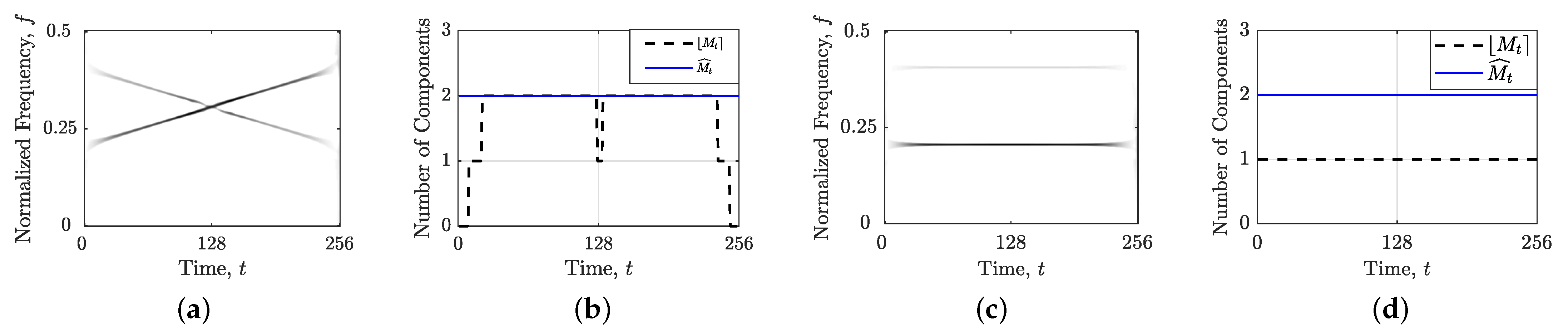
However, these global measures can be misleading for sparse TFDs because they may favor TFDs with fewer samples, falsely suggesting better performance by omitting important signal components [12,18,19,50]. To address this, the LRE method is used to recognize auto-terms, providing information about the local number of signal components. This involves comparing Rényi entropies of signal and reference components within each time and frequency slice, named as the short-term Rényi entropy (STRE) [26] and narrow-band Rényi entropy (NBRE) [18,19]:

$$M_t^{{\rho }_z(t,f)}\left(t_0\right)=2^{R\left({\chi }_{t_0}\left\{{\rho }_z(t,f)\right\}\right)-R\left({\chi }_{t_0}\left\{{\rho }_{\mathrm{ref}}(t,f)\right\}\right)},$$

(17)

$$M_f^{{\rho }_z(t,f)}\left(f_0\right)=2^{R\left({\chi }_{f_0}\left\{{\rho }_z(t,f)\right\}\right)-R\left({\chi }_{f_0}\left\{{\rho }_{\mathrm{ref}}(t,f)\right\}\right)},$$

(18)

where notations t and f indicate localization through time or frequency slices, respectively, $t_0$ and $f_0$ represent the observed time or frequency slice, respectively, while ${\rho }_{\mathrm{ref}}\left(t,f\right)$ is the reference QTFD. The operators ${\chi }_{t_0}$ and ${\chi }_{f_0}$ set to zero all TFD samples except those near $t_0$ (or $f_0$) [18,26]:

$${\chi }_{t_0}\left\{{\rho }_z(t,f)\right\}=\left\{\begin{array}{cc}{\rho }_z(t,f),\hfill & t\in [t_0-{\mathrm{\Theta }}_t/2,t_0+{\mathrm{\Theta }}_t/2],\hfill \\ 0,\hfill & \mathrm{otherwise},\hfill \end{array}\right.$$

(19)

$${\chi }_{f_0}\left\{{\rho }_z(t,f)\right\}=\left\{\begin{array}{cc}{\rho }_z(t,f),\hfill & f\in [f_0-{\mathrm{\Theta }}_f/2,f_0+{\mathrm{\Theta }}_f/2],\hfill \\ 0,\hfill & \mathrm{otherwise},\hfill \end{array}\right.$$

(20)

where ${\mathrm{\Theta }}_t$ and ${\mathrm{\Theta }}_f$ control the window lengths [18,26]. Note that the chosen reference signal in the NBRE is perfectly time-localized and covers all frequencies, contrasting with the STRE reference signal [18,19,26].

The authors in [18] combined mean squared errors (MSEs) between the original and reconstructed TFDs by using the LRE method as [18]:

$$\begin{array}{c}\hfill \mathrm{MSE}={\displaystyle \frac{1}{N_t}}\sum _{t=1}^{N_t}{\left({\displaystyle \frac{M_t^{{\rho }_z(t,f)}\left(t\right)-M_t^{{\mathsf{{\rm Y}}}_z^{{\mathsf{\ell }}_1}(t,f)}\left(t\right)}{max\left(M_t^{{\rho }_z(t,f)}\left(t\right),M_t^{{\mathsf{{\rm Y}}}_z^{{\mathsf{\ell }}_1}(t,f)}\left(t\right)\right)}}\right)}^2+\\ \hfill +{\displaystyle \frac{1}{N_f}}\sum _{f=1}^{N_f}{\left({\displaystyle \frac{M_f^{{\rho }_z(t,f)}\left(f\right)-M_f^{{\mathsf{{\rm Y}}}_z^{{\mathsf{\ell }}_1}(t,f)}\left(f\right)}{max\left(M_f^{{\rho }_z(t,f)}\left(f\right),M_f^{{\mathsf{{\rm Y}}}_z^{{\mathsf{\ell }}_1}(t,f)}\left(f\right)\right)}}\right)}^2,\end{array}$$

(21)

and formulated a state-of-the-art measure that can indicate if the TFD is overly sparse and lacks consistent auto-terms. Then, the optimal regularization parameter is determined by using the multi-objective optimization problem formulated as:

$$\min \{M_z^S,\mathrm{MSE}\},\mathrm{s}.\mathrm{t}.\lambda \in \langle 0,10],$$

(22)

where $M_z^S$ and MSE are minimized [18]. However, in the multi-objective optimization, improving one objective often degrades another [51,52,53,54]. This is also true for this use case, i.e., artificially the best $M_z^S=0$ is connected with the worst $\mathrm{MSE}=1$. Thus, the multi-objective algorithm constructs all feasible solutions in the Pareto front [51,52,53].

Meta-heuristic optimization algorithms are effective for non-linear optimization problems, handling non-differentiable, non-continuous, and non-convex objective functions. As in [18], the multi-objective particle swarm optimization method (MOPSO) [51,52,53] is utilized, which optimizes particle velocities, ${\left[V_z\right]}^{[n+1]}$, and positions, ${\left[x_z\right]}^{[n+1]}=\left[\lambda \right]$, based on individual and global best positions [51]:

$$\begin{array}{cc}\hfill {\left[V_z\right]}^{[n+1]}& =w·{\left[V_z\right]}^{\left[n\right]}+c_1{r}_1({\left[P_z\right]}^{\left[n\right]}-{\left[x_z\right]}^{\left[n\right]})+c_2{r}_2({\left[G_z\right]}^{\left[n\right]}-{\left[x_z\right]}^{\left[n\right]}),\hfill \\ \hfill [x_z{]}^{[n+1]}& ={\left[x_z\right]}^{\left[n\right]}+{\left[V_z\right]}^{[n+1]},\hfill \end{array}$$

(23)

where w is the inertia coefficient, $r_1$ and $r_2$ are random numbers in $[0,1]$, and $c_1$ and $c_2$ are cognitive and social components [51,52]. MOPSO incorporates Pareto dominance for optimal solutions, stored in the repository. Furthermore, the MOPSO involves an additional mutation operator in each iteration controlled by the mutation rate $m_r$ [51,52]. The final solution is selected using the fuzzy satisfying method [18]. This approach represents the current state-of-the-art technique for automatically optimizing regularization parameter, applied in various algorithms within CS-based sparse TFD reconstruction [16,18,21].

Limitations of the Current Meta-Heuristic Optimization Technique

Despite advantages, several limitations of the meta-heuristic approach [18] are addressed with this research. Objective functions of meta-heuristic optimization inherit limitations of the LRE method which can be imprecise for certain signal cases. Such signal examples are shown in Figure 1. For instance, an estimated local number of components exhibit drop at and in the vicinity of the crossing point in the TF plane of two or more components, as seen in Figure 1a,b. Furthermore, the LRE may not detect weaker component in a simple case with two parallel constant FM components, as seen in Figure 1c,d. In both cases, optimization can wrongly converge to an overly sparse TFD with lost auto-terms.

Meta-heuristic multi-objective optimization, despite its effectiveness, has several inherent limitations. A primary challenge is achieving an optimal balance between exploration and exploitation, which, if not adequately managed, can result in suboptimal solutions and slow convergence rates. Furthermore, these algorithms are typically computationally intensive, requiring substantial processing time and resources, especially when applied to complex, high-dimensional problems like the one addressed in this study. The performance of these algorithms is also highly sensitive to the selection of parameters and operators, which are often problem-specific. This specificity limits the generalizability of the approach and complicates the tuning process. Additionally, meta-heuristic methods generally lack a guarantee of identifying the true Pareto-optimal front, often resulting in approximations that may overlook critical solutions.

3. The Proposed Deep Neural Network-Based Approach for Determining Regularization Parameter

In this study, a novel approach is proposed for determining the regularization parameter $\lambda$ by training a neural network to learn a mapping from observations to regularization parameters. The mapping is defined as $\mathbf{\Phi }:{\mathbb{R}}^m\to {\mathbb{R}}^p$, where an input vector $\mathit{i}\in {\mathbb{R}}^m$ (the observations) is mapped to a vector $\mathit{\lambda }\in {\mathbb{R}}^p$ (the regularization parameters):

$$\mathit{\lambda }=\mathbf{\Phi }\left(\mathit{i}\right).$$

(24)

Here, the goal is to estimate the observation-to-regularization mapping function $\mathbf{\Phi }$ by approximating it with a neural network and learning its parameters $\mathit{\theta }$. DNNs are used for their universal approximation capabilities [37].

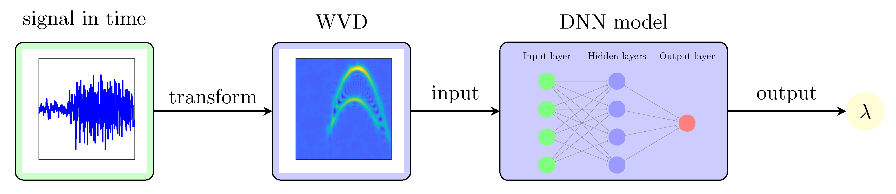
In this work, the DNN takes the WVD, represented in matrix form as ${\mathit{W}}_{\mathit{z}}$, which is calculated for input signal. Note that the WVD should be presented in its original form, without any post-processing. This choice offers several advantages. Firstly, the WVD can be computed efficiently for any signal and does not include any parameter, making it a straightforward input. Secondly, the WVD clearly delineates the spatial positions and amplitude discrepancies of auto-terms and cross-terms in the TF plane. Thirdly, using the WVD aligns well with the CS-based reconstruction method used in this work, which originates from its AF. A simplified block diagram of the proposed idea is illustrated in Figure 2.

The output of the DNN, denoted as $\widehat{\mathit{\lambda }}\left(\mathit{\theta }\right)$, is given by:

$$\widehat{\mathit{\lambda }}\left(\mathit{\theta }\right)=\widehat{\mathbf{\Phi }}({\mathit{W}}_{\mathit{z}};\mathit{\theta }).$$

(25)

For training the DNN, we determine the optimal regularization parameter values, denoted as ${\mathbf{\lambda }}_{\mathrm{opt}}$, for each provided WVD by minimizing the ${\mathsf{\ell }}_2$ norm between the ideal TFD, ${\mathit{\rho }}_{\mathrm{ideal}}$, and the reconstructed TFD using the YALL1 algorithm:

$${\mathit{\lambda }}_{\mathrm{opt}}=\underset{\mathit{\lambda }}{argmin}\left|\right|{\mathsf{{\rm Y}}}_z\left(\mathit{\lambda }\right)-{\mathit{\rho }}_{\mathrm{ideal}}{\left|\right|}_2.$$

(26)

The training data, denoted as ${\{{\mathit{W}}_{\mathit{z}}^{\left(j\right)},{\mathit{\lambda }}_{\mathrm{opt}}^{\left(j\right)}\}}_{j=1}^J$, comprises $J=$ 10,000 synthetic signal examples, both single and multi-component, expressed as a summation of M finite-duration signals:

$$z\left(t\right)=\sum _{m=1}^M{z}_m\left(t\right)\mathrm{\Pi }\left({\displaystyle \frac{t-\frac{t_{0_m}+t_{f_m}}{2}}{T_m}}\right)=\sum _{m=1}^M{z}_m\left(t\right){\mathrm{\Pi }}_m\left(t\right),$$

(27)

where $t_{0_m}$, $t_{f_m}$, and $T_m$ denote the starting time, ending time, and duration of the m-th signal component, respectively. Here, ${\mathrm{\Pi }}_m\left(t\right)$ is a rectangular function defined as:

$${\mathrm{\Pi }}_m\left(t\right)=\left\{\begin{array}{cc}1,\hfill & \left|t\right|\le T_m/2,\hfill \\ 0,\hfill & \mathrm{otherwise}.\hfill \end{array}\right.$$

(28)

Considering the common presence of LFM or QFM behavior in real-world signals [1,46,55], the m-th component $z_m\left(t\right)$ embodies either an LFM or QFM behavior, expressed as:

$$z_m^{\left(\mathrm{LFM}\right)}=A_m{e}^{2j\pi \left(B_m{t}^2+f_{0_m}t\right)},$$

(29)

$$z_m^{\left(\mathrm{QFM}\right)}=A_m{e}^{2j\pi \left(D_m{t}^3+C_m{t}^2+f_{0_m}t\right)},$$

(30)

where $f_{0_m}$ and $A_m$ are the starting normalized frequency and amplitude, respectively, and $B_m$, $C_m$, and $D_m$ are the frequency modulation rates. These parameters were randomly generated to encapsulate diverse variations of signal components across the entirety of the TFD, including instances of multiple intersections with varying amplitudes. Therefore, $t_{0_m},t_{f_m}\in [1,N_t]$, $f_{0_m}\in [0,0.5]$.

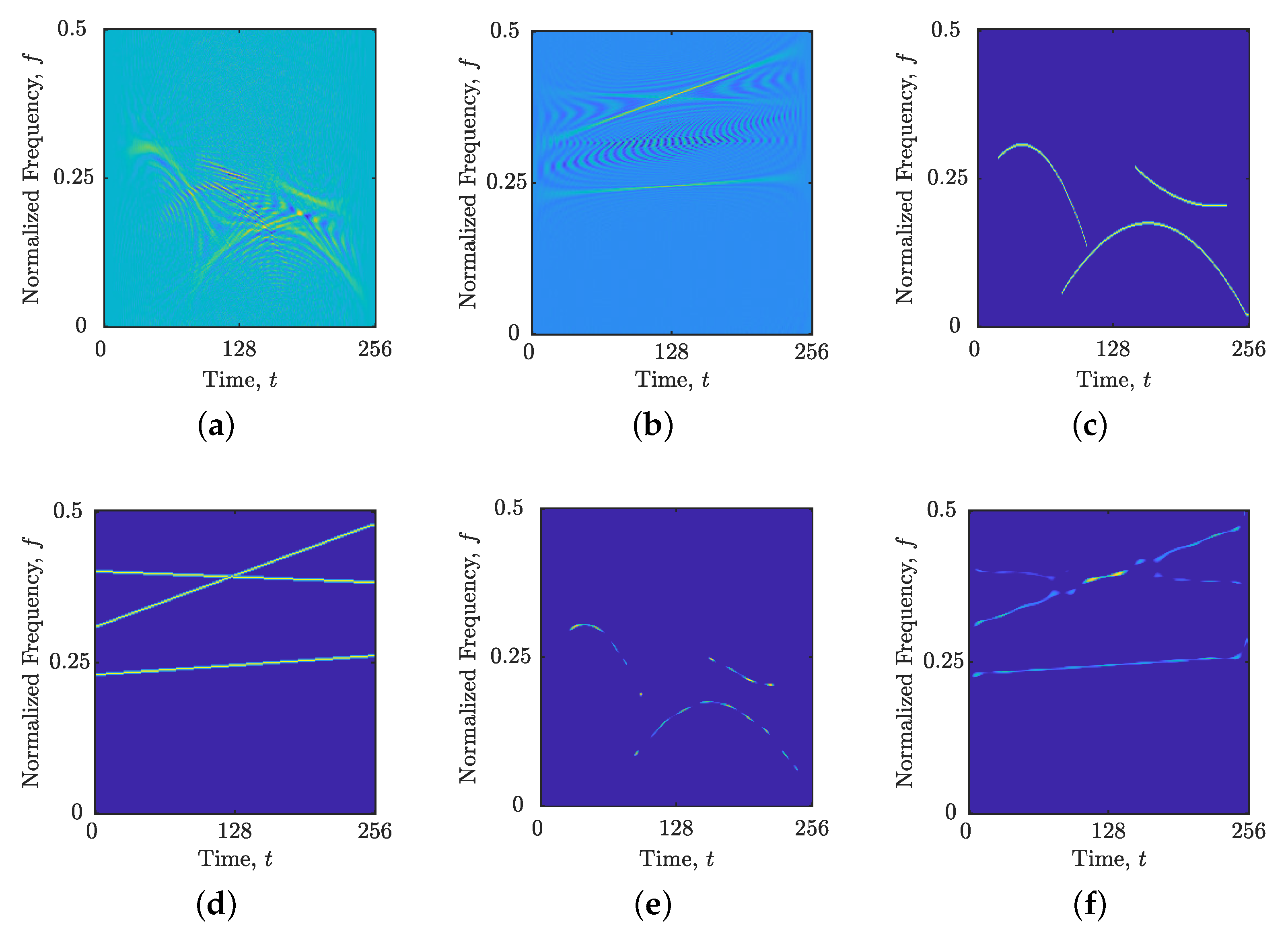
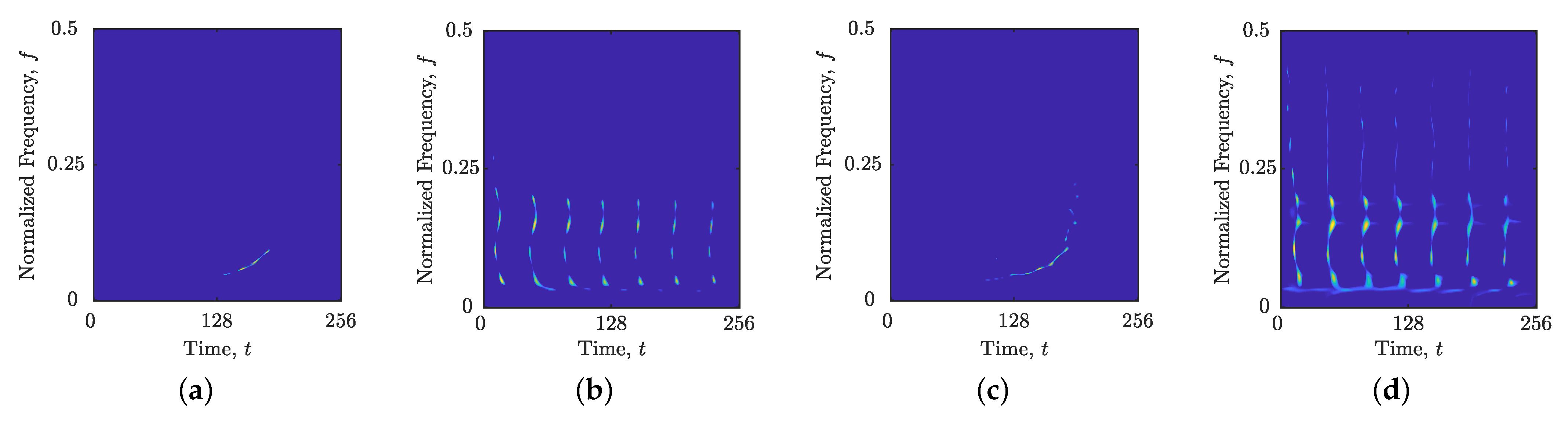
To account for real-world conditions, randomly selected signals were embedded into AWGN with a signal-to-noise (SNR) ratio as low as 0 dB, covering both noise-free and noisy scenarios. Additionally, the training signals were normalized relative to their maximum amplitude, necessitating the same normalization process when computing reconstructed TFDs for new signals using the regularization parameter predicted by the proposed DNN. As example, Figure 3 displays the WVDs, ideal TFDs and optimally reconstructed TFDs obtained using the YALL1 with $\lambda$ optimized by (26) for two synthetic signals from the training set. Note that the WVDs serve as inputs to the DNN, while the optimal ${\lambda }_{\mathrm{opt}}=3.10$ and ${\lambda }_{\mathrm{opt}}=1.60$ are stored in the output vector ${\mathit{\lambda }}_{\mathrm{opt}}$.

3.1. DNN Architectures

In this study, four DNN architectures are considered: a fully connected neural network (FCNN), ResNet, DenseNet, and a CNN with attention mechanisms. The FCNN uses a flattened layers, i.e., vectorized WVD as input, which simplifies the data representation and reduces computational complexity. However, this flattening process leads to a loss of spatial relationships of signal auto-terms and cross-terms within the TF plane, potentially hindering the model’s ability to capture patterns that are useful for accurate predictions. ResNets, with their skip connections, offer a solution by preserving spatial hierarchies and preventing the vanishing gradient problem in deep networks, making them highly effective in maintaining performance as the network depth increases. DenseNets further build on this by ensuring that each layer receives direct input from all preceding layers, promoting feature reuse and reducing the risk of overfitting. This architecture is particularly advantageous for tasks where capturing fine-grained spatial details is crucial. CNNs with attention mechanisms, such as Squeeze-and-Excitation (SE) blocks, enhance the model’s ability to focus on the most relevant regions of the matrix, dynamically adjusting to emphasize the most informative features. This makes attention-based CNNs particularly powerful for tasks requiring precise localization and analysis of patterns within large matrices. Overall, while FCNNs offer simplicity and computational efficiency, ResNets, DenseNets, and attention-based CNNs provide more sophisticated approaches that are better suited for capturing the complex spatial dependencies inherent in the TF plane, making them highly advantageous for tasks involving large matrix inputs.

Table 1. Architectures of deep neural networks used.

Model	Architecture
FCNN	Flatten(256x256), Dense(1024, ReLU), BatchNorm, Dropout(0.5), Dense(512, ReLU), BatchNorm, Dropout(0.5), Dense(256, ReLU), BatchNorm, Dropout(0.5), Dense(128, ReLU), Dense(1, ReLU)
ResNet	Conv2D(32, 3x3, ReLU, Input: 256x256x1), BatchNorm, MaxPool(2x2), Conv2D(64, 3x3, ReLU), BatchNorm, MaxPool(2x2), Conv2D(128, 3x3, ReLU), BatchNorm, MaxPool(2x2), Residual Block: [Conv2D(128, 3x3, ReLU) → BatchNorm → Conv2D(128, 3x3, ReLU) → BatchNorm → Add(Input)], Flatten, Dense(1, ReLU)
DenseNet	Conv2D(32, 3x3, ReLU, Input: 256x256x1), BatchNorm, MaxPool(2x2), Dense Block 1: [Conv2D(32, 3x3, ReLU) → BatchNorm → Concat], MaxPool(2x2), Dense Block 2: [Conv2D(64, 3x3, ReLU) → BatchNorm → Concat], MaxPool(2x2), Dense Block 3: [Conv2D(128, 3x3, ReLU) → BatchNorm → Concat], GlobalAvgPool, Dense(1, ReLU)
CNN with Attention	Conv2D(32, 3x3, ReLU, Input: 256x256x1), BatchNorm, MaxPool(2x2), Conv2D(64, 3x3, ReLU), BatchNorm, MaxPool(2x2), Conv2D(128, 3x3, ReLU), BatchNorm, MaxPool(2x2), Attention Block: [Conv2D(128, 1x1, ReLU) → Softmax(Channels) → Multiply(Input)], Flatten, Dense(1, ReLU)

outlines the architectures of each DNN used in this study.

The output layer (i.e., predicted $\lambda$) comprises a single neuron employing the ReLU activation function for regression predictions. To estimate $\theta$, ADAM optimized with a dynamic learning rate of $[{10}^{-5},{10}^{-1}]$ is utilized with the mean squared error loss function. The DNN models are trained on the input–output pairs for a maximum of 1000 epochs with a batch size of 32 and a validation split of 20%. To mitigate the risk of overfitting and ensure that proposed models generalize well to unseen data, an early stopping criterion is employed during training. Specifically, the early stopping mechanism monitors the validation loss and stops the training process if there is no improvement in the validation loss for 10 epochs. Additionally, it is ensured that the model reverts to the state where it achieved the best validation performance, rather than continuing to train and potentially overfitting to the training data.

3.2. Summary of the Proposed DNN-Based Approach

A general review of the proposed approach is outlined in Algorithm 1. In the offline phase, the training data are used to learn the DNN parameters. This involves computing multiple WVDs and reconstructed TFDs to find ${\mathit{\lambda }}_{\mathrm{opt}}^{\left(j\right)}$ for each synthetic signal. However, once the DNN is trained, forward propagation of the new signals through the network requires only the signal’s WVD. The obtained $\lambda$ using the DNN is finally used in the YALL1 algorithm in order to compute reconstructed TFD.

Algorithm 1 Reconstructed TFDs obtained via DNN.

offline phase:     generate J training signals, following by their WVDs ${\mathit{W}}_{\mathit{z}}^{\left(j\right)}$ and ideal TFDs ${\mathit{\rho }}_{\mathrm{ideal}}^{\left(j\right)}$, for $j=1,\dots ,J$     obtain ${\mathit{\lambda }}_{\mathrm{opt}}^{\left(j\right)}$ using (26)     use training data ${\{{\mathit{W}}_{\mathit{z}}^{\left(j\right)},{\mathit{\lambda }}_{\mathrm{opt}}^{\left(j\right)}\}}_{j=1}^J$ to compute DNN’s optimal parameters $\widehat{\mathit{\theta }}$

online phase:     compute WVD of the considered signal ${\mathit{W}}_{\mathit{z}}$     propagate ${\mathit{W}}_{\mathit{z}}$ through the learned network to get $\widehat{\mathit{\lambda }}\left(\mathit{\theta }\right)=\widehat{\mathbf{\Phi }}({\mathit{W}}_{\mathit{z}};\widehat{\mathit{\theta }})$     compute the reconstructed TFD ${\widehat{\mathsf{{\rm Y}}}}_z\left(\widehat{\mathit{\lambda }}\right)$ using YALL1

4. Experimental Results and Discussion

4.1. Experiment Setup

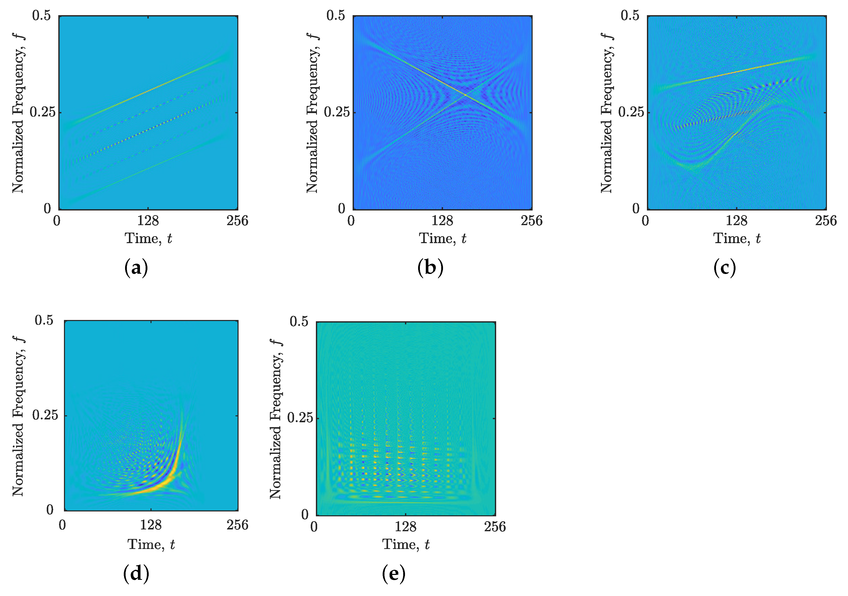
The proposed DNN-based approach performance was assessed on three synthetic signals with $N_t=256$ samples. Namely, $z_{\mathrm{S}1}\left(t\right)$ composed of three LFM components with different amplitudes: $z_{\mathrm{S}1}\left(t\right)=e^{j2\pi \left(0.00039t^2\right)}+0.5e^{j2\pi (0.1t+0.00039t^2)}+1.5e^{j2\pi (0.2t+0.00039t^2)}$; $z_{\mathrm{S}2}\left(t\right)$ composed of two crossing LFM components embedded in AWGN with $\mathrm{SNR}=4$ dB: $z_{\mathrm{S}2}\left(t\right)=0.9e^{j2\pi (0.1t+0.00059t^2)}+e^{j2\pi (0.45t-0.00049t^2)}$; and $z_{\mathrm{S}3}\left(t\right)$ composed of one LFM and one sinusoidal component embedded in AWGN with $\mathrm{SNR}=5$ dB: $z_{\mathrm{S}3}\left(t\right)=e^{j2\pi (0.3t+0.0002t^2)}+e^{j(0.38\pi t+23.04(sin(0.0245t-\pi /2)+1\left)\right)}$. Furthermore, the experiment was extended with real-world gravitational (this research has made use of data, software, and/or web tools obtained from the LIGO Open Science Center (https://losc.ligo.org), a service of LIGO Laboratory and the LIGO Scientific Collaboration. LIGO is funded by the U.S. National Science Foundation), $z_{\mathrm{G}}\left(t\right)$ [12,16,56,57], and EEG seizure signal, $z_{\mathrm{EEG}}\left(t\right)$ [12,50,58,59,60,61,62,63] as examples. For $z_{\mathrm{G}}\left(t\right)$, consisting of 3441 samples, downsampling by a factor of 14 resulted in $N_t=256$ samples, corresponding to a duration of 0.25 to 0.45 seconds and a frequency range of $[0,512]$ Hz. For $z_{\mathrm{EEG}}\left(t\right)$, a differentiator filter was applied to enhance its spike signatures as in [60,61,64,65]. Figure 4 illustrates the WVDs of the analyzed signals, highlighting the presence of cross-terms and noise contamination.

The CS-AF areas, $N_{\tau }^{\prime }\times N_{\nu }^{\prime }$, for the considered signals $z_{\mathrm{S}1}\left(t\right)$, $z_{\mathrm{S}2}\left(t\right)$, $z_{\mathrm{S}3}\left(t\right)$, $z_{\mathrm{G}}\left(t\right)$ and $z_{\mathrm{EEG}}\left(t\right)$ were calculated as $89\times 15$, $17\times 15$, $27\times 15$, $35\times 19$, and $15\times 15$, respectively. For the MOPSO, the parameters were configured as follows: a maximum of 50 iterations, a population size of 25, and 25 particles in the repository. The coefficients were set to $w=0.9,c_1=c_2=2,m_r=0.1$, as used in [18]. The reconstruction algorithm parameters were set as $N_{it}=200$ and $ϵ={10}^{-3}$ following the recommendations in [11,12,14,16,18,19]. The LRE computation used ${\alpha }_R=3$ and ${\mathrm{\Theta }}_t={\mathrm{\Theta }}_f=11$ as recommended in [12,21,26,66]. The simulations of the algorithms’ execution times, averaged over 1000 independent runs, have been performed on a PC with the Ryzen 7 3700X @ 3.60GHz Base Clock processor and 32GB of DDR4 RAM.

The reconstruction performance has been evaluated using machine learning evaluation metrics [67]. The use of these metrics has proven effective in image and signal processing, as demonstrated in previous studies [55,68,69,70]. To apply these metrics, the reconstructed and ideal TFDs were converted into a binary classification framework. Here, the positive class (P) denotes the presence of signal auto-term samples in the TFD, whereas the negative class (N) indicates the absence of signal. The ideal TFD contains true samples that should precisely match their positions and classifications in the reconstructed TFD. Consequently, the following metrics were employed: true positives (TPs)—samples correctly identified as the positive class, true negatives (TNs)—samples correctly identified as the negative class, false positives (FPs)—samples incorrectly categorized in the positive class, and false negatives (FNs)—samples incorrectly categorized in the negative class [67]. A high FP value suggests the inclusion of noise and/or cross-term-related samples in the reconstruction, while a high FN value indicates missing true signal samples in the reconstructed TFD.

These metrics are visually summarized in a confusion matrix [67,71]. Based on the confusion matrix and its components, several statistical measures are calculated [67]:

$$\mathrm{Accuracy}={\displaystyle \frac{\mathrm{TP}+\mathrm{TN}}{\mathrm{TP}+\mathrm{TN}+\mathrm{FP}+\mathrm{FN}}},$$

(31)

$$\mathrm{Precision}={\displaystyle \frac{\mathrm{TP}}{\mathrm{TP}+\mathrm{FP}}},$$

(32)

$$\mathrm{Recall}={\displaystyle \frac{\mathrm{TP}}{\mathrm{TP}+\mathrm{FN}}},$$

(33)

$$\mathrm{F}1\mathrm{score}=2·{\displaystyle \frac{\mathrm{Precision}·\mathrm{Recall}}{\mathrm{Precision}+\mathrm{Recall}}}={\displaystyle \frac{2·\mathrm{TP}}{2·\mathrm{TP}+\mathrm{FP}+\mathrm{FN}}}.$$

(34)

All these statistical metrics range from 0 to 1, with higher values indicating better performance.

4.2. Performance of DNN Architectures

Considering the MAE metric provided in

Table 2. Comparison of MAE values for different DNN architectures. Bolded values highlight the best-performing architecture.

Model	Training MAE	Validation MAE
FCNN	0.0960	0.1318
ResNet	0.0794	0.1011
DenseNet	0.0830	0.1026
CNN with Attention	0.0919	0.0956

, the CNN with attention achieves the lowest validation MAE of 0.0956, reflecting its superior ability to generalize to unseen data. In comparison, DenseNet and ResNet follow with validation MAEs of 0.1026 and 0.1011, respectively, demonstrating competitive generalization capabilities. The FCNN, with the highest validation MAE of 0.1318, underperforms due to the loss of spatial information resulting from the input WVD being flattened. Furthermore, the FCNN reached overfitting more quickly, completing training in 90 epochs, while ResNet, DenseNet, and CNN with attention utilized 105, 155, and 170 epochs, respectively. Training times for FCNN, ResNet, DenseNet, and CNN with attention are 2.85, 3.53, 4.56, and 26.73 hours, respectively. For tasks where prediction accuracy is critical and resources are available, the CNN with attention is the best choice due to the best validation MAE. Otherwise, ResNet and DensNet provide better balance between architecture complexity and performance. Consequently, the ResNet (further in the text as the proposed DNN) is selected in this study for further analysis due to its lower training time with competitive training and validation MAEs.

4.3. Comparison with the Current Meta-Heuristic Optimization Approach

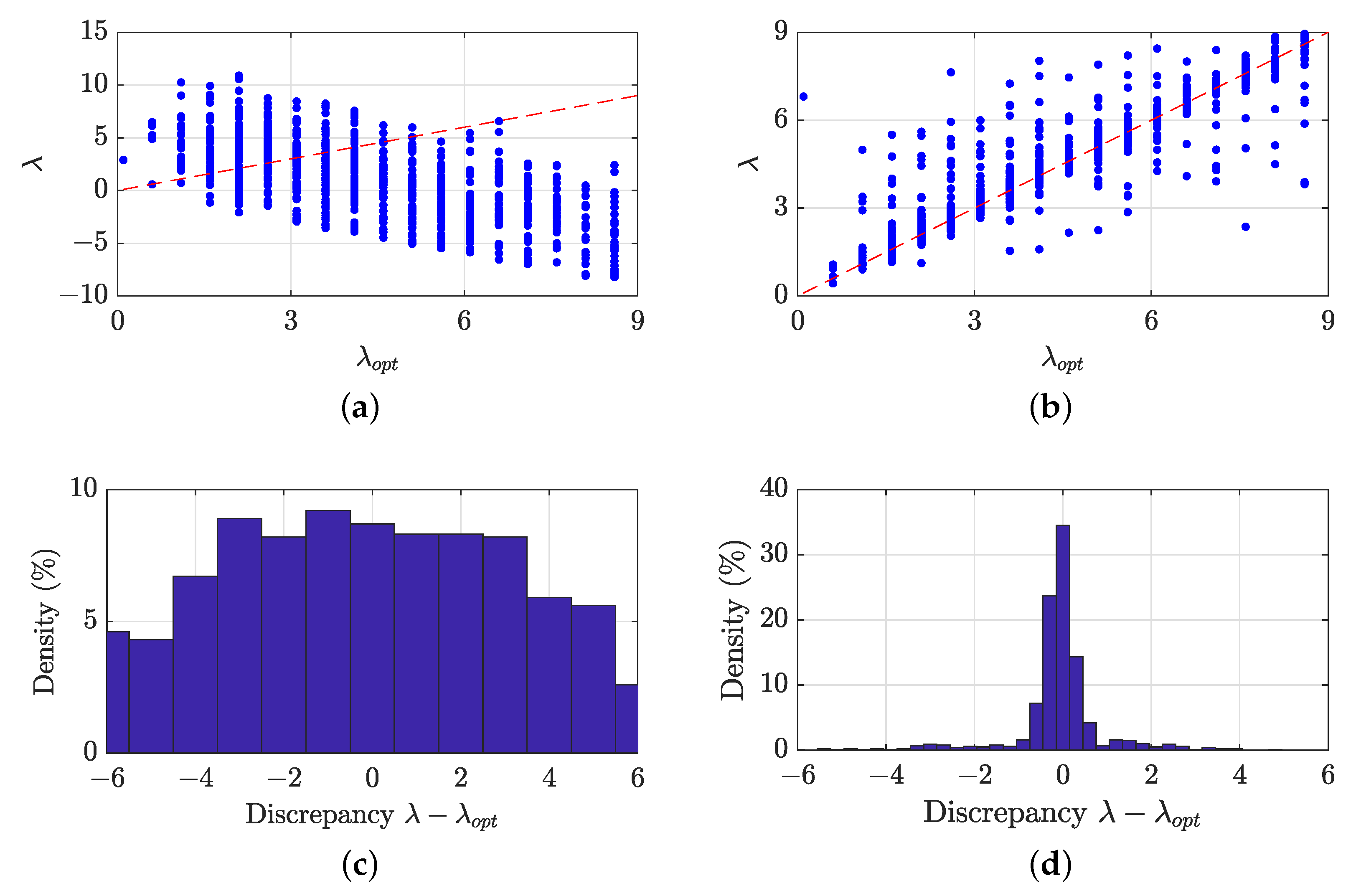
The performance of the DNN in predicting regularization parameters compared to those obtained using the existing MOPSO approach is visualized in Figure 5. Specifically, the scatter plot for the DNN (see Figure 5b) indicates a better correlation between the optimal and predicted regularization parameters compared to the MOPSO predictions (see Figure 5a). This improvement is further illustrated in the density plots for the discrepancy $\lambda -{\lambda }_{\mathrm{opt}}$. The density plot for the DNN, shown in Figure 5d, reveals that most discrepancies between the optimal and DNN-predicted regularization parameters are within $\pm 1$. In contrast, the density plot for the MOPSO, shown in Figure 5c, exhibits roughly equal probabilities for discrepancies up to $\pm 3$, with only a slight decrease for discrepancies in continuation. This suggests that MOPSO optimization using the LRE is less reliable, potentially becoming trapped in local optima or converging to a suboptimal TFD reconstruction due to LRE limitations.

Figure 6 and Figure 7 present the reconstructed TFDs obtained using the YALL1 with DNN-based versus LRE-based MOPSO $\lambda$ parameter. Across all considered synthetic and real-world signal examples, the DNN-based reconstructed TFDs demonstrate performance competitive with those obtained via MOPSO. Notably, the DNN-based reconstructed TFDs maintain high-resolution auto-terms while effectively suppressing cross-terms and noise, visually outperforming the MOPSO-based reconstructed TFDs. Given that auto-terms reconstructed by the YALL1 often appear discontinuous, the LRE-based MOPSO approach [18] tends to mitigate this discontinuity but at a cost. To maintain the computed number of components in each time and frequency slice, MOPSO optimization (i) reduces the resolution of auto-terms and (ii) leaves cross-terms or noise samples to fill in the gaps, as illustrated in Figure 6b,c. Furthermore, when the LRE fails to accurately detect components with low amplitude, the reconstructed TFD does not preserve these components well, as seen in Figure 6a.

Additionally, the auto-terms of real-world signals $z_{\mathrm{G}}\left(t\right)$ and $z_{\mathrm{EEG}}\left(t\right)$ are not fully preserved when using MOPSO, as depicted in Figure 7. This occurs because of two reasons. First, the LRE does not detect auto-terms with lower amplitude. Second, more samples, even those related to auto-terms, artificially degrade the objective $M_z^S$ measure, consequently favoring oversparse reconstructed TFDs. By visually inspecting reconstructed TFDs with $\lambda$ predicted by the DNN in Figure 7, they exhibit better preservation of auto-terms, indicating that the training data used in this study can be used for analyzing unseen real-world signals featuring LFM and/or QFM components, as in $z_{\mathrm{G}}\left(t\right)$ and $z_{\mathrm{EEG}}\left(t\right)$.

The numerical performance comparison of the DNN-based and LRE-based MOPSO reconstructed TFDs (shown in Figure 6) with the ideal TFDs are presented in

Table 3. Performance comparison of reconstructed TFDs obtained using the YALL1 algorithm with $\lambda$ parameter optimized via MOPSO with LRE [18] versus the proposed DNN for the signals $z_{\mathrm{S}1}\left(t\right)$, $z_{\mathrm{S}2}\left(t\right)$, and $z_{\mathrm{S}3}\left(t\right)$. Values in bold indicate superior reconstructed TFD for each signal.

			${\mathit{z}}_{\mathbf{S}1}\left(\mathit{t}\right)$		${\mathit{z}}_{\mathbf{S}2}\left(\mathit{t}\right)$		${\mathit{z}}_{\mathbf{S}3}\left(\mathit{t}\right)$
			${\mathrm{{\rm Y}}}_z(t,f)$		${\mathrm{{\rm Y}}}_z(t,f)$		${\mathrm{{\rm Y}}}_z(t,f)$
			N	P	N	P	N	P
MOPSO-LRE	${\rho }_{\mathrm{ideal}}(t,f)$	N	62,725	253	62,410	1343	62,892	852
		P	1464	838	866	661	1025	511
ineDNN	${\rho }_{\mathrm{ideal}}(t,f)$	N	62,564	414	63,594	159	63,490	254
		P	1358	944	1127	400	1134	402
ine			MOPSO-LRE	DNN	MOPSO-LRE	DNN	MOPSO-LRE	DNN
Accuracy			0.9737	0.9729	0.9662	0.9803	0.9712	0.9787
Precision			0.7681	0.6951	0.3298	0.7156	0.3749	0.6128
Recall			0.3640	0.4101	0.4329	0.2620	0.3327	0.2617
F1 score			0.4940	0.5158	0.3744	0.3835	0.3525	0.3668
Execution time (obtaining $\lambda$ + YALL1), t [s]			7788 + 4.17	0.0598 + 4.12	7911 + 3.84	0.0591 + 3.89	7889 + 3.94	0.0609 + 3.97

. Overall, the results validate the visual observations mentioned above. For the signal $z_{\mathrm{S}1}\left(t\right)$, the DNN-based reconstructed TFD achieves better preservation of the auto-terms with lower amplitude than the MOPSO-based one. This is indicated by higher TP and lower FN indices in the confusion matrix (and consequently higher recall), as more auto-term samples are correctly predicted with fewer samples falsely set to zero. On the other hand, given a higher $\lambda$, the MOPSO-based reconstructed TFDs exhibit higher TN and lower FP, achieving higher accuracy and precision metrics.

The opposite behavior can be observed for noise signals $z_{\mathrm{S}2}\left(t\right)$ and $z_{\mathrm{S}3}\left(t\right)$. Reconstruction of cross-term and noise-related samples using the MOPSO is indicated by a significant increase in FP and a decrease in TN indices compared with reconstruction using the DNN-predicted $\lambda$, which is also evident from lower accuracy and precision metrics. Consequently, in this case, the lower $\lambda$ obtained using MOPSO preserves more auto-term-related samples, as indicated by higher TP and lower FN indices, and higher recall metric. For all three synthetic signal examples, the DNN-predicted reconstructed TFDs exhibit superior F1 scores.

Some of the reported precision, recall, and F1 scores are relatively low, which can be attributed to several factors. In an ideal TFD that contains only auto-term maxima, positive samples represent a very small proportion of the total, resulting in a highly imbalanced dataset where the majority of samples are zero. This imbalance diminishes the reliability of accuracy as a standalone evaluation metric, highlighting the importance of using precision, recall, and F1 score metrics for a more comprehensive and reliable assessment. Several factors influence the reported metrics. While the YALL1 algorithm significantly enhances auto-term resolution and effectively suppresses interference, the reconstructed auto-term resolution is still less sharp than the ideal, and its trajectory may exhibit discontinuities. These discontinuities, while not affecting the extraction of useful information, can impact classification metrics. Additionally, the reconstruction process and initial interference may introduce slight biases in the positions of auto-term maxima within the reconstructed TFD, leading to deviations from their ideal locations. Another contributing factor is the presence of random TF samples with negligible amplitude in the TFD. If not thresholded, these insignificant samples can artificially lower the evaluation metrics. In this study, the focus has been on evaluating reconstructed TFDs without any post-processing, such as thresholding or over/under-sampling of the data. Future research will explore suitable post-processing methods and metrics to improve the performance and robustness of these classification metrics for this use case.

4.4. Computational Complexity

FCNN, ResNet, DenseNet, and CNN with attention consist 67,544,065, 4,908,673, 206,261, and 34,876,001 parameters, from which 67,540,481, 4,902,913, 201,853 and 34,872,545 are trainable, respectively. Calculating the full computational complexities of neural networks involves considering the number of operations required in each layer. These complexities are typically expressed in terms of the number of floating-point operations (FLOPs), which can be calculated based on the architecture of each network. The FCNN is the least intensive at approximately 67.8 million FLOPs due to its simpler architecture. In contrast, ResNet and DenseNet offer a balance between complexity and performance, with complexities of around 849.3 million FLOPs and 471.8 million FLOPs, respectively, making DenseNet slightly more efficient. The CNN with attention has the highest complexity at approximately 1.227 billion FLOPs due to the additional attention mechanisms.

The main motivation for using the DNN is in reducing the execution time for obtaining $\lambda$ in the online phase, which is significantly lower than performing full meta-heuristic optimization. As reported in Table 3, obtaining optimal $\lambda$ can take up to 7911 s using MOPSO, while the trained DNN gives its prediction in approximately 0.06 s, which is significantly faster. Indeed, execution time of the MOPSO can be improved by decreasing the numbers of particles and iterations. However, that may lead to more inaccurate $\lambda$ values and consequently reconstructed TFDs with worse performance. As it was intended in [12,18,50], meta-heuristic optimization should be used for offline signal analysis, while the proposed DNN approach is a perspective to be used even for online analysis.

4.5. Noise Sensitivity Analysis

To evaluate the impact of noise on the prediction of the $\lambda$ parameter by the proposed DNN, a comprehensive comparative analysis was conducted using precision, recall, and F1 score metrics. These metrics were derived from the comparison between the ideal TFDs and the noisy reconstructed TFDs obtained using DNN- or MOPSO-predicted $\lambda$. The synthetic signals were subjected to AWGN across four SNR levels ranging from 9 dB to 0 dB. The results, based on 1000 independent noise realizations, are summarized in

Table 4. Performance comparison of reconstructed TFDs obtained using YALL1 with $\lambda$ optimized via MOPSO with LRE [18] versus the proposed DNN for signals $z_{\mathrm{S}1}\left(t\right)$, $z_{\mathrm{S}2}\left(t\right)$, and $z_{\mathrm{S}3}\left(t\right)$ in AWGN with SNR $=[0,3,6,9]$ dB. Precision, recall, and F1 score values are averaged over 1000 noise realizations.

			MOPSO-LRE	DNN	MOPSO-LRE	DNN	MOPSO-LRE	DNN	MOPSO-LRE	DNN
			0 dB		3 dB		6 dB		9 dB
$z_{\mathrm{S}1}\left(t\right)$
$\overline{\mathrm{Precision}}$			0.2042	0.3356	0.3506	0.4512	0.4759	0.5004	0.6460	0.6788
$\overline{\mathrm{Recall}}$			0.2849	0.3188	0.3267	0.3678	0.3238	0.3787	0.3311	0.3888
$\overline{\mathrm{F}1\mathrm{score}}$			0.2321	0.3248	0.3330	0.3946	0.3821	0.4301	0.4301	0.4941
$z_{\mathrm{S}2}\left(t\right)$
$\overline{\mathrm{Precision}}$			0.2290	0.5866	0.3188	0.6588	0.3661	0.7222	0.4127	0.7325
$\overline{\mathrm{Recall}}$			0.2978	0.2211	0.3845	0.2509	0.4231	0.2801	0.4276	0.2898
$\overline{\mathrm{F}1\mathrm{score}}$			0.2588	0.3189	0.3401	0.3620	0.3888	0.3987	0.4088	0.4140
$z_{\mathrm{S}3}\left(t\right)$
$\overline{\mathrm{Precision}}$			0.2155	0.4325	0.3344	0.5878	0.4014	0.6255	0.4454	0.6328
$\overline{\mathrm{Recall}}$			0.2544	0.2144	0.3188	0.2544	0.3488	0.2878	0.3566	0.3011
$\overline{\mathrm{F}1\mathrm{score}}$			0.2301	0.2814	0.3164	0.3541	0.3701	0.3901	0.3944	0.4051

. The findings underscore the superiority of the DNN reconstructions over the MOPSO reconstructions for all synthetic signal examples. This superiority is discerned through higher F1 scores and precision metrics, particularly notable at lower SNR values.

4.6. Limitations of the Proposed Approach

While the proposed DNN approach exhibits strong predictive capabilities for estimating the regularization parameter in sparse time–frequency distributions of non-stationary signals, it does have certain limitations. The model’s effectiveness is sensitive to the type of noise present in the signals. For instance, in scenarios involving specific noise types such as impulsive or colored noise, retraining the network may be necessary to achieve optimal performance, as the current model is primarily designed for signals corrupted by AWGN. Additionally, the model may experience degraded performance when analyzing real-world signals that do not exhibit LFM or QFM components.

Moreover, although this network has been specifically trained using the YALL1 algorithm for sparse reconstruction, its deep learning architecture is sufficiently flexible to allow for straightforward retraining with other reconstruction algorithms. This adaptability enables the model to incorporate additional parameters beyond the regularization parameter $\lambda$, potentially enhancing its utility across a broader range of applications.

5. Conclusions

This study introduces a novel approach utilizing DNNs for predicting the regularization parameter in CS-based reconstruction of TFDs. By training the DNNs on synthetic signals composed of LFM and QFM components, the proposed method aims to eliminate the need for manual parameter selection or complex optimization procedures, which are often time-consuming, require specialist knowledge, and depend on appropriate objective functions.

The results demonstrate the efficacy of the DNN-based approach in automatically determining the regularization parameter, showing competitive performance compared to existing optimization methods in terms of reconstruction quality. Specifically, the DNN-based reconstructions better preserve auto-terms with low amplitude, exhibit high-resolution auto-terms, and effectively suppress cross-terms and noise. This has also been validated by real-world gravitational signal examples for which the proposed DNN was not specifically trained. Additionally, the DNN-based reconstructions are less sensitive to noise.

Two additional advantages of using DNNs over meta-heuristic optimization are emphasized. First, the end-user only needs to provide the signal’s WVD as input to the network, circumventing the limitations and parameter tuning of additional methods such as LRE and MOPSO. Second, obtaining the $\lambda$ parameter using a trained DNN is significantly faster than performing meta-heuristic optimization, suggesting that DNNs can be used for online application purposes.

Overall, this study highlights the potential of DNNs in automating the determination of regularization parameters for TFD reconstruction, paving the way for enhanced signal processing applications in diverse environments. Future research could explore the possibility of constructing the training data with application-specific signal types and noise conditions, as well as applying DNNs across different reconstruction algorithms and approaches. Furthermore, future research will include the development of adaptive regularization parameter using DNNs.