Automatic Segmentation and Statistical Analysis of the Foveal Avascular Zone

Abstract

This study facilitates the extraction of foveal avascular zone (FAZ) metrics from optical coherence tomography angiography (OCTA) images, offering valuable clinical insights and enabling detailed statistical analysis of FAZ size and shape across three patient groups: healthy, type II diabetes mellitus and both type II diabetes mellitus (DM) and high blood pressure (HBP). Additionally, it evaluates the performance of four deep learning (DL) models—U-Net, U-Net with DenseNet121, U-Net with MobileNetV2 and U-Net with VGG16—in automating the segmentation of the FAZ. Manual segmentation of the images by ophthalmological clinicians was performed initially, and data augmentation was used to enhance the dataset for robust model training and evaluation. Consequently, the original set of 103 full retina OCTA images was extended to 672 cases, including 42 images from normal patients, 357 images from DM patients, and 273 images from patients with both DM and HBP. Among the models, U-Net with DenseNet outperformed the others, achieving the highest accuracy, Intersection over Union (IoU), and Dice coefficient across all patient groups. This research is distinct in its focus on full retina OCTA images and its inclusion of patients with both hypertension and diabetes, an area that is less studied in the existing literature.

1. Introduction

Diabetic retinopathy (DR) remains the leading cause of blindness among working-age adults in developed countries, affecting approximately 93 million people worldwide [1]. This shows the substantial impact of diabetes on global vision health and illustrates the necessity for proactive screening and treatment to prevent significant vision loss. Similarly, hypertensive retinopathy (HR) is a major retinal condition, affecting an estimated 10–15% of people with high blood pressure (HBP) [2]. The occurrence of HR increases with age and the severity of hypertension, highlighting the importance of effective blood pressure control in reducing the risk of retinal damage. Together, DR and HR are among the most critical retinal vascular conditions, accentuating the importance of integrated healthcare approaches to effectively manage both diabetes and hypertension to prevent vision deterioration and other complications [3].

Optical coherence tomography angiography (OCTA), also known as Angio-OCT, is a modern, non-invasive, rapid, and side-effect-free technique used to analyze retinal and chorioretinal microvasculature. This advanced imaging method can detect early signs of both diabetic retinopathy (DR) and hypertension-related retinal changes. It can identify irregular edges of the foveal avascular zone (FAZ), small aneurysms that traditional eye exams might miss, and reduced surface blood vessel density, making it a valuable tool for early detection and management of these conditions.

OCTA has the capability to provide detailed imaging of both the deep and superficial retinal plexuses, as well as the full retina. While imaging the superficial and deep plexuses individually is valuable, using full retina imaging offers a comprehensive assessment of the retinal microvasculature across all layers of the retina.

Many studies have explored the changes in the FAZ area in different retinal diseases compared to healthy patients. These studies have demonstrated that the FAZ tends to remodel and enlarge in conditions like diabetic retinopathy, with a negative correlation observed between the FAZ area and visual acuity [4,5]. Additionally, other research has highlighted the significance of the acircularity index and axis ratio of the FAZ as crucial metrics for assessing retinal changes in patients with various pathologies [6]. However, these metrics have predominantly been analyzed within the deep or superficial retinal layers, rather than in the context of full retina OCTA images and have not been extensively studied in patients with diabetes and hypertension. Integrating artificial intelligence (AI) into the analysis of these metrics can enhance precision, automation, and scalability. AI’s ability to process large datasets of FAZ metrics from diverse patient populations enables the identification of emerging trends and correlations. This can provide ophthalmologists with valuable new insights into how diabetes and hypertension impact retinal health, enabling them to better understand the variations in disease progression and response to treatment among diverse patient groups.

This paper presents two significant contributions. First, it introduces an approach for generating FAZ metrics and binary masks from full retina OCTA images, enabling detailed statistical analysis of FAZ size and shape across three patient groups: healthy individuals, those with type II diabetes mellitus (DM), and those with both type II diabetes mellitus and high blood pressure (HBP). Second, it provides a comparative analysis of four advanced deep learning models—U-Net, U-Net with DenseNet121, U-Net with MobileNetV2, and U-Net with VGG16—assessing their effectiveness in reducing the manual workload for clinicians and their potential applications in clinical practice for FAZ segmentation.

2. Related Work

In recent years, advancements in technology have increasingly enabled the incorporation of specialized computer-aided diagnosis systems into the field of ophthalmology [7,8,9].

Recent advances in deep learning-based methods have significantly enhanced the accuracy and robustness of segmentation in retinal disease imaging [8,10,11,12,13,14]. According to [14], in a controlled test setting, DL models can match the accuracy of professional judgment in screening and diagnosing common vision-threatening conditions, including diabetic retinopathy (DR), glaucoma, age-related macular degeneration (AMD) and cataracts. Many of these studies reflect the growing use of automated systems to accurately measure key retinal parameters such as FAZ area, perimeter, acircularity index and axis lengths in patients with various retinal diseases, demonstrating their effectiveness in capturing FAZ shape changes associated with disease progression.

For example, one study [4] introduced a deep learning model using a convolutional neural network (CNN) for segmenting the FAZ in superficial end face OCTA images. This model, based on Detectron2, was compared to the device’s built-in software and manual measurements in both healthy and diabetic eyes. It achieved a high Dice similarity coefficient of 0.94, showing excellent correlation with manual measurements and outperforming the device’s software, particularly in diabetic eyes with macular edema. Another study [15] developed a fully automatic system for FAZ segmentation in superficial OCT-A images using a CNN. Validated on a dataset of 213 images from both healthy and diabetic eyes, the system achieved a correlation coefficient of 0.93 and a Jaccard index of 0.82 for healthy eyes, and a correlation coefficient of 0.93 and a Jaccard index of 0.83 for diabetic eyes. This tool provides objective and reproducible FAZ measurements, including area, perimeter, circularity index, and axis lengths, which are valuable for analyzing retinal microcirculation and diagnosing vascular diseases. Additionally, [16] developed an algorithm that combines a Hessian-based filter with a U-Net deep learning network for automatic FAZ segmentation. Using a dataset of 260 OCTA images, the algorithm achieved an 87.8% Jaccard Index, with 6% false-negative and 5% false-positive error rates. The results indicate that the U-Net network performs well in FAZ segmentation even with a small training set, and that Hessian-based filtering enhances accuracy. Another study [17] proposed a hybrid approach combining AI-based segmentation with machine learning to enhance the diagnostic accuracy of Alzheimer’s disease using FAZ analysis. OCTA data from 37 Alzheimer’s patients and 48 healthy controls were analyzed, with FAZ segmentation performed on the superficial capillary plexus. Multiple radiomic features (area, solidity, compactness, roundness, and eccentricity) were extracted and used alongside clinical variables in a light-gradient boosting machine algorithm. This method achieved an area under the curve (AUC) of 72.0 ± 4.8%, improving diagnostic performance by 14% compared to single-feature analysis, demonstrating the potential of combining multiple biomarkers and machine learning for more effective FAZ-based Alzheimer’s diagnosis. Also, a recent study [18] introduced a deep transfer learning-based system for real-time diabetic retinopathy (DR) detection using fundus cameras, addressing the challenges of high diagnostic costs and limited medical access in remote areas. The system uses a VGGNet, a deep learning algorithm, to analyze superficial retinal images captured by fundus cameras, effectively detecting and classifying the severity of DR. The system achieved a high classification accuracy of 97.6%, outperforming existing methods.

With highly advanced OCT devices, especially those equipped with spectral-domain OCT (SD-OCT) or swept-source OCT (SS-OCT) technology, clinicians can focus on different layers of the retina, such as the superficial (inner retina) and deep (outer retina) layers. Some of these devices also offer the ability to perform full retina thickness scans, which capture the entire thickness of the retina, from the inner limiting membrane (ILM) to the retinal pigment epithelium (RPE). Full retina imaging offers a comprehensive view of the entire retina [19], enabling the detection of multiple conditions, such as diabetic retinopathy and hypertension, in a single scan. According to [20], in diabetic retinopathy, vessel density reduction is most prominent in the deep capillary plexus, but it can also affect other retinal layers. In glaucoma, abnormalities are often observed in the superficial vascular complex of the optic nerve, while in retinitis pigmentosa, the macular deep capillary plexus is typically affected. The peripapillary circulation, located at the margin of the optic nerve head, is a critical site in the pathogenesis of retinal vein occlusion, optic disc rim (Drance) hemorrhage, and glaucoma [21,22]. Also, vessel density reduction can impact the full retina, including all retinal and choroidal layers, in conditions such as coronary heart disease [23], hypertension or Alzheimer’s [24]. Furthermore, when correlated with changes in the FAZ, full retina scans provide a more detailed and accurate assessment, enhancing the detection and monitoring of disease progression. Unfortunately, this approach presents challenges, including the need for high-resolution imaging, managing large volumes of data, and interpreting complex results. Successful integration of advanced technologies into clinical practice depends on interdisciplinary collaboration, with clinicians providing crucial medical insights, engineers enhancing the technology’s design and functionality, and data scientists analyzing extensive datasets to ensure the technology is both practical and advantageous for patient care.

3. Materials and Methods

The framework proposed in our study (Figure 1) offers a Python-based tool for extracting the FAZ binary masks and key metrics from full retinal OCTA images, such as area $A_1$, perimeter $P_1$, area and perimeter of the equivalent circle of FAZ ($A_2$, $P_2$), acircularity index (A_index), L_major axis of equivalent ellipse (blue), L_minor axis of equivalent ellipse (orange), angle (θ) and axis ratio (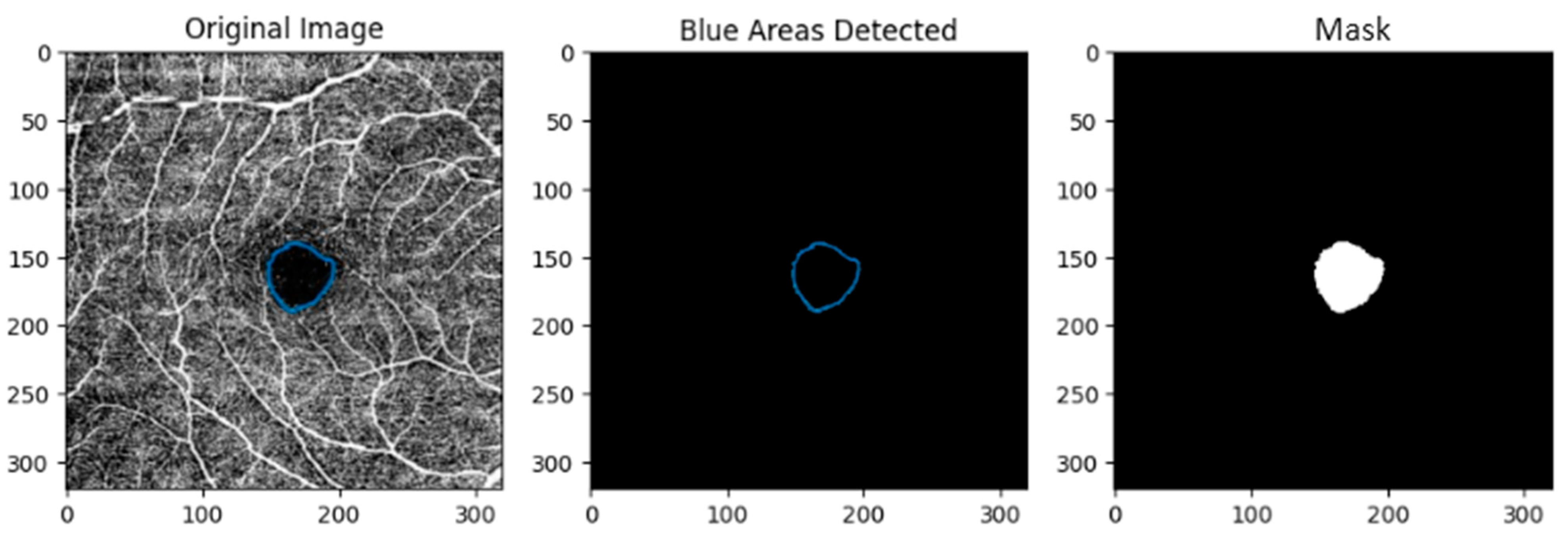A_ratio). This study involved three distinct patient groups: healthy individuals (Control/Normal), patients with type II diabetic mellitus (DM) and patients with both type II diabetes mellitus and high blood pressure (DM + HBP). Initially, OCTA images are manually segmented by clinicians to ensure precise FAZ metrics and binary mask generation. Next, the contour of the FAZ (highlighted in a blue distinct color, Figure 2) is detected, and the binary masks are generated. At the same time, the FAZ metrics are obtained in. csv files and provided to ophthalmologists for clinical statistical analysis, facilitating the investigation of correlations between FAZ morphology and patient-specific disease characteristics.

Additionally, four advanced deep learning models are evaluated to enable the FAZ binary mask generation, reducing the need for manual segmentation. The models are U-Net, U-Net with DenseNet121, U-Net with MobileNetV2, and U-Net with VGG16. As shown in Section 4, in the testing phase, U-Net with DenseNet achieves the highest scores in terms of accuracy, Intersection over Union (IoU), and Dice coefficient across all patient groups during the testing phase: 98.73%, 82.50% and 90.41% in the case of the Normal group; 97.97%, 83.07% and 90.75% in the case of the DM group; and 97.46%, 80.90% and 88.94% in the case of the DM + HBP group.

3.1. Proposed Framework

The framework proposed in our study is illustrated in Figure 1. This represents an interdisciplinary effort that integrates medical expertise with AI engineering techniques to facilitate the clinical assessment of foveal avascular zone measurements from full retina OCTA images in healthy individuals, patients with type II diabetes mellitus, and those with both type II diabetes mellitus and hypertension. This approach provides ophthalmologists with valuable new information and clinical insights, enabling more precise diagnosis and treatment planning. Moreover, our study is built on an open-source Python foundation, fostering opportunities for further research and collaboration. The key steps of our research are as follows:

• The OCTA image dataset was provided by clinicians from the Department of Ophthalmology at Clinical Emergency County Hospital “Sf. Ap. Andrei” Galați, in accordance with the exclusion criteria outlined in the Section 3.2. The dataset comprises 103 OCTA images obtained from 82 individual patients. This larger-than-patient count image dataset is due to the multiple scans taken per patient for a more thorough evaluation. Some patients had both eyes imaged, while others had repeat scans at varying time points or angles on the same eye, which helps in capturing subtle, time-dependent vascular and retinal changes. These multiple captures ensure that the study addresses intra- and inter-eye variations as well as longitudinal changes in retinal structure.
• Manual segmentation of FAZ was performed by clinicians on 103 OCTA images to ensure precise measurement and mask generation. Each of the 103 images underwent careful manual segmentation by clinicians to ensure high accuracy in measuring the FAZ. This labor-intensive process generated reliable segmentation masks for the FAZ in each image, which form a trusted baseline that is crucial for validating automated segmentation techniques. This multi-faceted dataset allows a comprehensive view of the FAZ metrics under varying conditions, making it particularly valuable for training and evaluating AI models in medical imaging.
• A Python-based algorithm was designed to detect the contours (boundaries of the FAZ marked by clinicians) in order to extract FAZ binary mask and metrics—area A₁, perimeter P₁, area and perimeter of the equivalent circle of FAZ (A₂, P₂), acircularity index (A_index), major axis (L_major) of equivalent ellipse, minor axis (L_minor) of equivalent ellipse, angle (θ) and axis ratio (A_ratio). FAZ metrics are saved in CSV format for each patient group.
• The statistical analysis of FAZ metrics was conducted by clinicians to assess the data for each patient group.
• The original set of 103 full retina OCTA images was augmented to a total of 672 cases: 42 images from healthy patients, 357 images from diabetes mellitus patients, and 273 images from patients with both type II diabetes mellitus and high blood pressure (HBP).
• Comparison between four advanced DL models (U-Net, U-Net with Dense121, U-Net with MobileNetV2 and U-Net with VGG16) to fully automate the process of FAZ extraction.

As illustrated in Figure 1, full retina OCTA images from each patient group are manually segmented by ophthalmologists and subsequently processed using a Python-based algorithm that extracts the ground-truth masks of the FAZ. Based on these masks, the FAZ metrics are determined, and clinicians can perform statistical analyses to investigate the relationships between vascular density, FAZ characteristics, and systemic conditions. This methodology provides critical insights into how these factors influence retinal microvascular health.

Furthermore, the full retina OCTA images, along with their corresponding ground-truth masks, indicated by the two arrows, are used to evaluate four DL models—U-Net, U-Net with DenseNet121, U-Net with MobileNetV2 and U-Net with VGG16. According to the findings presented in the Section 4, U-Net with DenseNet121 demonstrates the best performance. This model has the potential to replace manual segmentation and FAZ mask extraction, thereby fully automating the process of determining the FAZ metrics.

3.2. Dataset

With the approval of Clinical Emergency County Hospital “Sf. Ap. Andrei” Galați, Department of Ophthalmology, 82 patients were selected for evaluation during the period of 2021–2022. Patients were chosen based on specific inclusion and exclusion criteria. The inclusion criteria included age over 18 years, healthy patients, those with a diagnosis of type II diabetes mellitus or both type II diabetes mellitus and essential hypertension. The healthy patients were identified through clinical assessments and a thorough review of their medical history to confirm the absence of any systemic conditions, such as type II diabetes or high blood pressure.

To ensure accurate results, the exclusion criteria included:

• Presence of signs of diabetic retinopathy (DR) during fundus examination.
• Other cardiovascular conditions.
• Ocular media opacities, such as corneal leukoma, mature cataract, or vitreous hemorrhage.
• Surgical interventions on the anterior or posterior segment of the eye performed less than 6 months prior to study inclusion.
• Other congenital or degenerative retinal conditions.

The ophthalmological evaluation of each patient included determination of visual acuity; refractometry to establish refractive error; biomicroscopy of the anterior and posterior segments and determination of intraocular pressure; and Angio-OCT.

The OCT angiography images were acquired using the advanced Topcon 3D OCT-1 Maestro II imaging system after pupil dilation with Tropicamide 5 mg/mL. Based on the ETDRS grid, a 6 × 6 mm area of the macula was scanned. The device’s software generated images of the superficial retina, deep retina, choriocapillaris, and full retina. Additionally, the device automatically determined the central vascular density at the level of the superficial capillary plexus.

The analyzed images were those of the full retina. While full retina images were obtained from both eyes, only the image from the eye with the highest quality was used for analysis. Patients whose images had poor signal quality or multiple artifacts that hindered clear delineation of the FAZ were excluded from the study.

The selected patients were divided into groups based on their diagnosis: healthy patients, those with type II diabetes, and those with both type II diabetes and essential hypertension. The groups were matched for demographic characteristics, including age, gender, and place of residence. All patients provided informed consent before their inclusion in the study. This study adheres to ethical standards in accordance with the principles of the Declaration of Helsinki and was approved by the Ethics Committee of the College of Physicians in Galați (Approval No. 398/11 April 2024).

3.3. Foveal Avascular Zone

3.3.1. Manual Segmentation and Mask Extraction

A total of 103 full retina OCTA images were segmented manually by clinicians. Next, for each image, the corresponding binary mask (Figure 2) was generated with a Python-based algorithm (version 3.10.12—OpenCV, Numpy, Matplotlib and Pandas libraries) that can detect the section marked with a distinct blue color.

The steps of the Python-based algorithm are:

• Step 1: Load Images: The marked image is loaded using cv2.imread().
• Step 2: Color Space Conversion: The marked image is converted to the HSV color space using cv2.cvtColor().
• Step 3: Color Detection: A specific shade of blue is targeted using a predefined BGR color converted to HSV. A mask is created to isolate this blue color within the image.
• Step 4: Contour Detection: Contours are found in the blue mask using cv2.findContours().
• Step 5: Binary Mask: A binary mask corresponding to the detected blue area is created.
• Step 6: FAZ Metrics: The metrics are determined with the formulas from the Section 3.3.2 and stored in CSV files for each patient group.

3.3.2. Metrics

The FAZ metrics obtained in this study are area $A_1$, perimeter $P_1$, area and perimeter of the equivalent circle of FAZ ($A_2$, $P_2$), acircularity index (A_index), major axis (L_major) of equivalent ellipse, minor axis (L_minor) of equivalent ellipse, angle (θ) and axis ratio (A_ratio).

A perfectly circular FAZ has an acircularity index (A_index) of 1. The acircularity index is calculated as the ratio between the FAZ perimeter $P_1$ and the perimeter $P_2$ of the equivalent circle of the FAZ:

$$A\_index={\displaystyle \frac{P_1}{P_2}}$$

(1)

Ellipse fitting is used to determine the major axis, minor axis, and angle (θ) of the FAZ. The axis ratio (A_ratio) is defined as the ratio between the major and minor axis of an equivalent ellipse of FAZ:

$$A\_ratio={\displaystyle \frac{L\_major}{L\_minor}}$$

(2)

3.3.3. Statistical Analysis

In this section, the statistical analysis of FAZ metrics performed by clinicians with IBM SPSS Statistics 21 is detailed for three groups: control group (6 images), type II diabetes mellitus (56 images), and type II diabetes mellitus with high blood pressure (HBP) (41 images).

The statistical tests used in this analysis include the Kruskal–Wallis H Test and the Spearman Correlation Coefficient.

The Kruskal–Wallis H test, a nonparametric method, was used to assess significant differences among two or more independent groups when the dependent variable is continuous or ordinal. The formula is:

$$H={\displaystyle \frac{12}{N(N+1)}}\sum _{i=1}^k{\displaystyle \frac{R_i^2}{n_i}}-3(N+1)$$

(3)

where $N$ = total number of observations across all groups; $k$ = number of groups; $n_i$ = number of observations in group $i$; $R_i$ = sum of ranks for group $i$.

The Spearman correlation coefficient measures the strength and direction of a monotonic relationship between two ranked variables, making it valuable for analyzing non-linear associations in medical data where variables may not follow a normal distribution. In statistical analysis, the Spearman coefficient is especially useful when exploring relationships in metrics such as FAZ (foveal avascular zone) characteristics and central vascular density (DVF C), as it highlights any consistent associations across patient groups, even in smaller, real-world sample sizes.

This approach provides insight into how closely variations in one variable (e.g., FAZ area) are associated with changes in another (e.g., DVF C) without assuming linearity. Values range from −1 to 1, with values closer to ±1 indicating stronger correlations, and significance is typically assessed using p-values. The formula is:

$$\rho =1-{\displaystyle \frac{6\sum d_i^2}{n(n^2-1)}}$$

(4)

where $d_i$ = difference between the ranks of observations; $n$ = number of observations.

The data are reported with a 95% confidence level and a margin of error of ±5%. A p-value of less than 0.05 was deemed statistically significant.

3.4. Deep Learning Models

To fully automate the process of FAZ extraction, we evaluated the performance of four deep learning models: U-Net, U-Net variant with Dense121, U-net variant with MobileNetV2, and U-Net variant with VGG16. The architectures of the models are illustrated in Figure 3, Figure 4, Figure 5 and Figure 6. We designed and configured these models to address the challenges of FAZ extraction, a critical area in the retina characterized by the absence of blood vessels. Accurate segmentation of the FAZ is essential for diagnosing and monitoring various retinal diseases, including those related to hypertension, diabetic retinopathy, and macular degeneration.

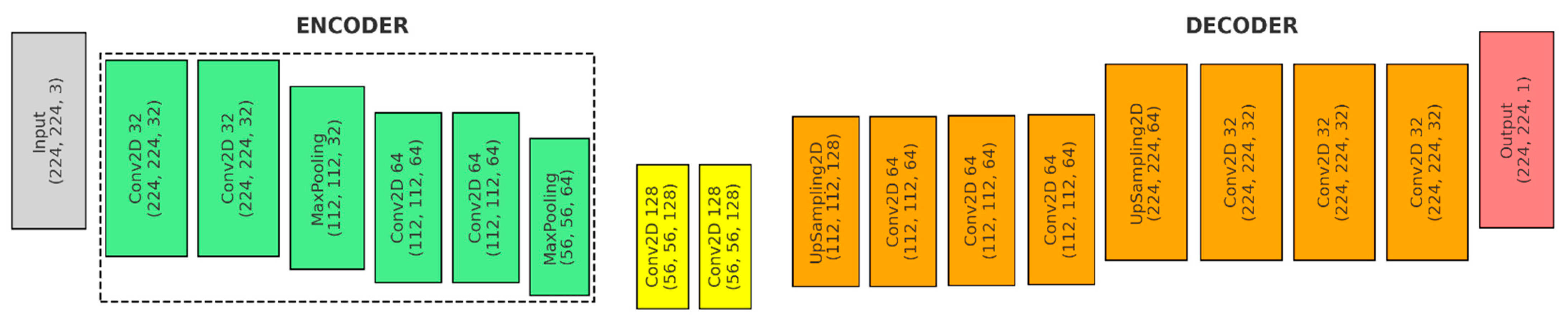
Figure 3 shows the first model, the U-Net architecture with an encoder–bottleneck–decoder structure designed to accept input images with a shape of input_shape, typically 224 × 224 × N pixels:

(a)

Input: The input shape is (224, 224, 3).

(b)

Encoder (Green): The encoder consists of a series of convolutional layers followed by max-pooling layers, which progressively downsample the spatial dimensions while increasing the depth of the feature maps.

●

Convolutional Layers: Each downsampling block in the encoder consists of two convolutional layers. The first block uses 32 filters, and the second block uses 64 filters. Each convolutional layer uses a 3 × 3 kernel, ReLU activation, and ‘same’ padding.

●

Pooling Layers: After each set of convolutional layers, a max pooling layer is used to reduce the spatial dimensions.

(c)

Bottleneck (Yellow): The bottleneck layer in a U-Net architecture is the deepest part of the network, where the feature maps have the smallest spatial dimensions but the highest number of channels.

●

Convolutional Layers: The bottleneck consists of two convolutional layers, each with 128 filters and a 3 × 3 kernel.

(d)

Decoder (Orange):

●

1st Upsampling Block: An upsampling layer—UpSampling2D(size = (2, 2)), a convolutional layer with 64 filters and a 2 × 2 kernel—Conv2D(64, (2, 2)), a skip connection and merging operation—concatenate([conv2, up4], axis = 3), and two convolutional layers with 64 filters and a 3 × 3 kernel—Conv2D(64, (3, 3)).

●

2nd Upsampling Block: An upsampling layer—UpSampling2D(size = (2, 2)), a convolutional layer with 32 filters and a 2 × 2 kernel—Conv2D(32, (2, 2)), a skip connection and merging operation—concatenate([conv1, up5], axis = 3), and two final convolutional layers with 32 filters and a 3 × 3 kernel—Conv2D(32, (3, 3)).

(e)

Output (Red): Produces a single-channel feature map with dimensions of 224 × 224 × 1.

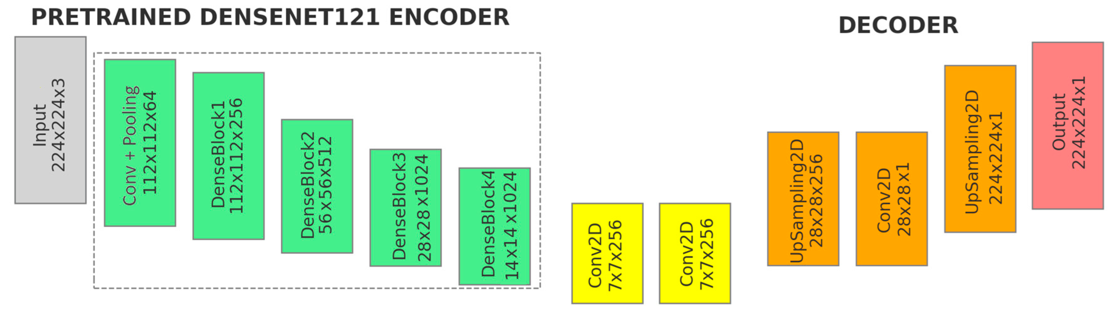
Figure 4 illustrates the second model, the U-Net variant with DenseNet121 backbone pre-trained on ImageNet:

(a)

Input: The input shape is (224, 224, 3).

(b)

Pretrained DenseNet121 Encoder (Green): Includes the initial convolution and pooling layers, followed by the four dense blocks of the DenseNet121 backbone.

(c)

Additional Convolutional Layers (Yellow): The feature maps from the DenseNet121 backbone (encoder) are passed directly into additional convolutional layers.

●

1st Convolutional Layers: Applies 256 filters with a 3 × 3 kernel, padding ‘same’ and use_bias = False − Conv2D(256, (3, 3)).

●

2st Convolutional Layers: Consists of 256 filters, a 3 × 3 kernel, padding ‘same’ and use_bias = False − Conv2D(256, (3, 3)).

●

After each convolutional layer, batch normalization, ReLU activation, and a 0.1 dropout are applied to stabilize the training process and enhance learning efficiency.

(d)

Decoder (Orange):

●

Upsampling Layer—UpSampling2D(size = (4, 4)): The feature maps are upsampled by a factor of 4 using bilinear interpolation. This increases the spatial resolution of the feature maps, reversing the downsampling that occurred in the encoder.

●

Final Convolutional Layer—Conv2D(1, (1, 1)): 1 × 1 Convolution, producing a single-channel output with ‘sigmoid’ activation.

●

Final Upsampling Layer: The final upsampling operation adjusts the spatial dimensions of the output to match the original input image size. This ensures that the segmentation mask aligns correctly with the input image.

(e)

Output (Red): The output of the model is a single-channel feature map (224, 224, 1).

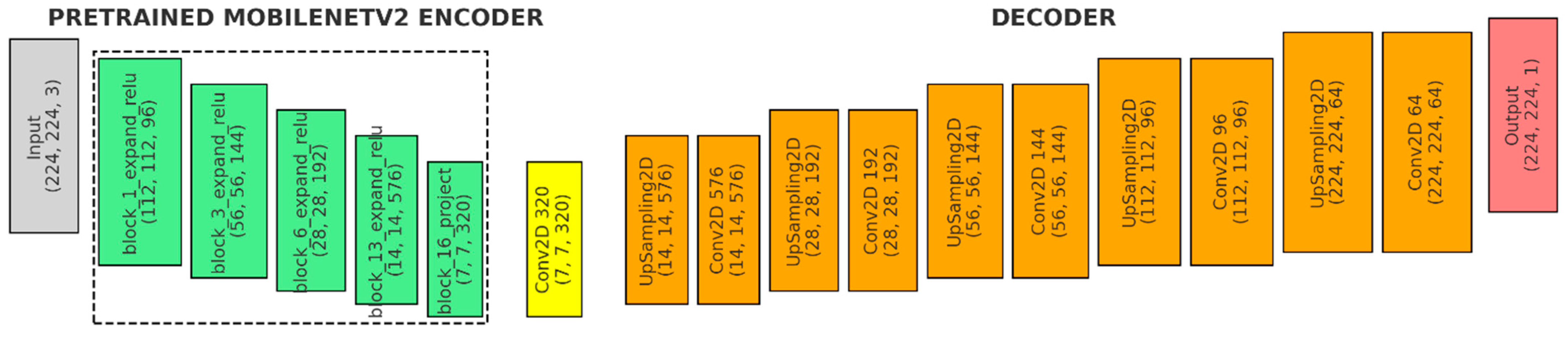
Figure 5 shows the third model, the U-Net variant with MobileNetV2 backbone, pre-trained on ImageNet:

(a)

Input (Gray): The input shape is defined as (224, 224, 3).

(b)

Pretrained MobileNetV2 Encoder (Green): The encoder uses the MobileNetV2 model with pre-trained weights, excluding the fully connected layers at the top (include_top = False). It captures outputs from five key blocks within MobileNetV2, each representing different stages of feature extraction with varying spatial resolutions and depths.

(c)

Bridge Layer (Yellow): This convolutional layer processes the deepest features (block5_pool) from the MobileNetV2 backbone. It facilitates the transition from the encoder to the decoder, preparing the feature maps for the upsampling process.

(d)

Decoder (Orange):

●

1st Upsampling stage: An upsampling layer with size = (2, 2) − UpSampling2D((2, 2), a 576-filter convolutional layer with a 3 × 3 kernel, ReLU activation, and ‘same’ padding (Conv2D(576, (3, 3))), followed by a skip connection to the corresponding encoder layer, batch normalization and a 0.3 dropout.

●

2nd Upsampling stage: An upsampling layer with size = (2, 2) − UpSampling2D((2, 2), a 192-filter convolutional layer (3 × 3 kernel, ReLU, ‘same’ padding) − Conv2D(192, (3, 3), a skip connection, batch normalization and a 0.3 dropout.

●

3rd Upsampling stage: An upsampling layer with size = (2, 2) − UpSampling2D((2, 2), a 144-filter convolutional layer (3 × 3 kernel, ReLU, ‘same’ padding) − Conv2D(144, (3, 3), a skip connection, batch normalization, and a 0.3 dropout.

●

4th Upsampling stage: An upsampling layer with size = (2, 2) − UpSampling2D((2, 2), a 96-filter convolutional layer (3 × 3 kernel, ReLU, ‘same’ padding) − Conv2D(96, (3, 3), a skip connection, batch normalization, and a 0.3 dropout.

●

5th Upsampling stage: An upsampling layer with size = (2, 2) − UpSampling2D((2, 2), a 64-filter convolutional layer (3 × 3 kernel, ReLU, ‘same’ padding) − Conv2D(64, (3, 3), followed by batch normalization before the final output.

(e)

Output (Red): A Conv2D layer with a 1 × 1 kernel, a single filter, sigmoid activation, and ‘same’ padding.

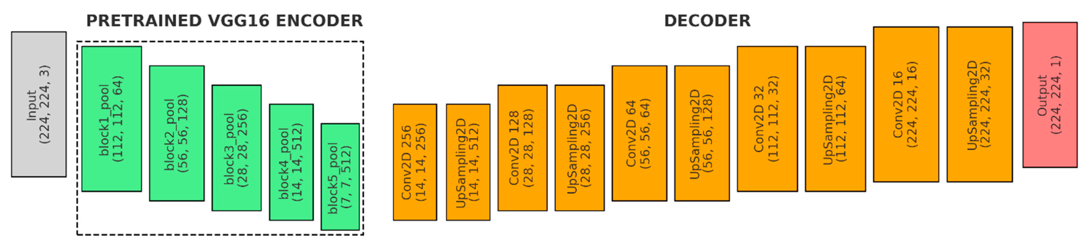
Figure 6 shows the fourth model, the U-Net variant with VGG16 backbone, pre-trained on ImageNet:

(a)

Input (Gray): The input shape is (224, 224, 3).

(b)

Encoder (Green): Loads the VGG16 model, which is pre-trained on the ImageNet dataset. The fully connected layers at the top of VGG16 are excluded (include_top = False).

●

Freezing Layers: The convolutional layers of VGG16 are frozen, meaning their weights will not be updated during training. This is common to retain the pre-learned features while adding new layers for specific tasks.

(c)

Decoder (Orange):

●

1st Upsampling Stage: A Conv2D layer with 256 filters (3 × 3 kernel, ReLU, ‘same’ padding), followed by UpSampling2D to double the spatial dimensions and a skip connection to VGG16’s block4_pool feature map.

●

2nd Upsampling Stage: A Conv2D layer with 128 filters (3 × 3 kernel, ReLU, ‘same’ padding), UpSampling2D with size = (2, 2), and a skip connection to VGG16’s block3_pool feature map.

●

3rd Upsampling Stage: A Conv2D layer with 64 filters (3 × 3 kernel, ReLU, ‘same’ padding), UpSampling2D with size = (2, 2), and a skip connection to VGG16’s block2_pool feature map.

●

4th Upsampling Stage: A Conv2D layer with 32 filters (3 × 3 kernel, ReLU, ‘same’ padding) and UpSampling2D to double the spatial dimensions.

●

5th Upsampling Stage: A Conv2D layer with 16 filters (3 × 3 kernel, ReLU, ‘same’ padding) and UpSampling2D with size = (2, 2).

(d)

Output (Red): 1 × 1 Convolutional layer with ‘sigmoid’ activation and ‘same’ padding to reduce the depth of the feature map to 1.

All neural network models were compiled using the Adam optimizer with a learning rate of 0.0001, binary cross-entropy as the loss function, and accuracy as the evaluation metric. Each model was trained for 50 epochs with a batch size of 8, using the training and validation datasets. The data were split into 80% for training and validation, and 20% for testing. Hyperparameters were optimized through Grid Search, which systematically explored a range of values to find the optimal configuration that maximized validation performance.

To evaluate the neural networks’ ability to segment the FAZ area, we assessed their performance on the test dataset using pixel accuracy (Equation (5)), IoU (Intersection over Union—Equation (6)), and the Dice coefficient (Equation (7)) [25]. The formulas are:

$$\mathrm{P}\mathrm{i}\mathrm{x}\mathrm{e}\mathrm{l} \mathrm{A}\mathrm{c}\mathrm{c}\mathrm{u}\mathrm{r}\mathrm{a}\mathrm{c}\mathrm{y}={\displaystyle \frac{TP+TN}{TP+TN+FN+FP}}$$

(5)

where TP = True Positives (correctly predicted positives—correctly identified as belonging to the target), TN = True Negatives (correctly predicted negatives—pixels correctly identified as not belonging to the target), FP = False Positives (incorrectly predicted positives—pixels incorrectly identified as belonging to the target) and FN = False Negatives (incorrectly predicted negatives—pixels incorrectly identified as not belonging to the target).

$$\mathrm{I}\mathrm{o}\mathrm{U}={\displaystyle \frac{\left|P\cap G\right|}{\left|P\cup G\right|}}$$

(6)

where P = set of pixels in the predicted segmentation, G = set of pixels in the ground truth segmentation, $\left|P\cap G\right|$ = pixels that are in both the predicted segmentation and the ground truth (TP), and $\left|P\cap G\right|$ = pixels that are in between predicted segmentation and ground truth.

$$\mathrm{D}\mathrm{i}\mathrm{c}\mathrm{e}={\displaystyle \frac{2\left|P\cap G\right|}{\left|P\right|+\left|G\right|}}$$

(7)

where P = set of pixels in the predicted segmentation, G = set of pixels in the ground truth segmentation, $\left|P\cap G\right|$ = pixels that are in between predicted segmentation and ground truth, $\left|P\right|$ and $\left|G\right|$ = the total number of pixels in the predicted and ground truth regions.

The results, detailed in the Section 4, show the performance metrics achieved for each group: healthy patients (Normal/Control), type II DM, and type II DM + HBP. Data augmentation with OpenCV Python functions (including clockwise and counterclockwise rotations of 30° and 60°, as well as horizontal and vertical flipping) and resizing to 224 × 224 pixels were applied to enhance the dataset for model training and evaluation. Consequently, the original set of 103 full retina OCTA images was extended to a total of 672 cases: 42 images from healthy patients, 357 images from diabetes mellitus patients, and 273 images from patients with both type II diabetes mellitus and high blood pressure (HBP).

4. Results and Discussion

This section presents statistical analyzes of FAZ metrics obtained from a total of 103 OCTA images, such as FAZ area $A_1$, FAZ perimeter $P_1$, equivalent circle of FAZ perimeter $P_2$, acircularity index (A_index), angle (θ) of FAZ and axis ratio (A_ratio) determined with a Python-based algorithm that is able to detect the marked contour of FAZ and extract its binary mask.

The decision to limit the patient sample size to fewer than 100 was due to the constraints of working with real-world clinical data. Patient consent, availability, and strict inclusion criteria were crucial for ensuring high-quality data relevant to the study. Despite a smaller sample size, AI methods yielded reliable diagnostic results, supported by rigorous statistical analysis.

Analyses included non-parametric methods, such as boxplot metrics, the Kruskal–Wallis H test, and Spearman correlation, which identified significant differences in FAZ metrics and relationships with central vascular density. These analyses achieved statistical significance even with fewer participants, underscoring the reliability of the AI model in differentiating key FAZ indicators across patient groups. The combined use of AI and statistical validation ensures that findings are robust, clinically relevant, and indicative of meaningful patterns and relationships in FAZ metrics, which could support clinical decision making.

Figure 7, Figure 8, Figure 9, Figure 10, Figure 11 and Figure 12 collectively provide valuable insights into the correlations between various FAZ metrics—such as area ($A_1$), perimeter ($P_1$), equivalent circle perimeter ($P_2$), acircularity index (A_index), angle (θ), and axis ratio (A_ratio)—and systemic conditions, including type II diabetes and high blood pressure, across the three patient groups. Figure 7, Figure 8 and Figure 9 show how these metrics correlate with disease progression and changes in retinal structure, while Figure 10, Figure 11 and Figure 12 further explore the relationship between Central Vascular Density (DVF C) and FAZ morphology. Central Vascular Density is a quantitative metric used in modern OCTA technology to assess the blood vessel density in the central area of the retina, typically around the FAZ. It quantifies the concentration of blood vessels within this region, which can be indicative of vascular health and is commonly analyzed in OCTA imaging. Variations in DVF C can signal abnormalities related to diabetic retinopathy, hypertension, or other retinal conditions, making it a key metric in ophthalmological diagnostics.

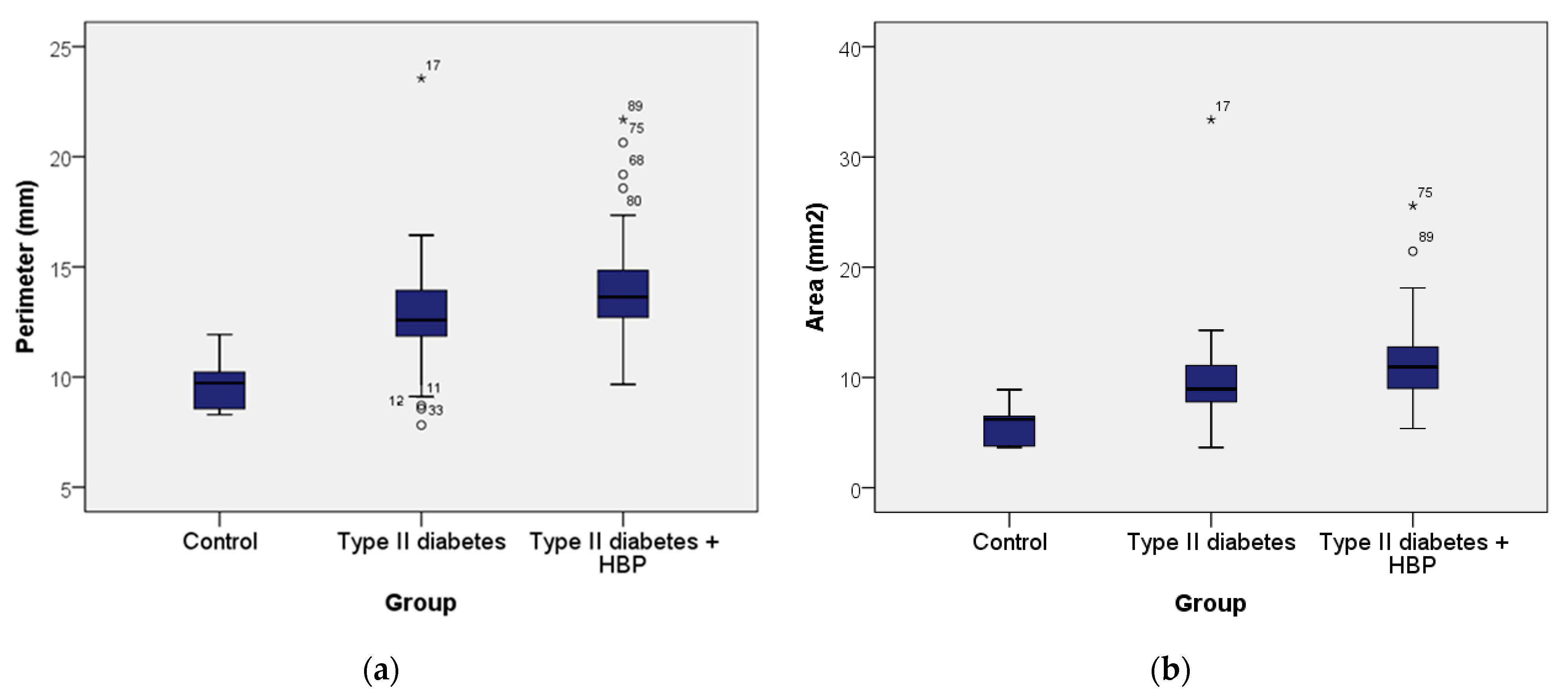
Figure 7 shows the boxplots of FAZ perimeter ($P_1$) and area ($A_1$). In Figure 7a, the control group shows a FAZ perimeter ranging from 8.29 to 11.93 mm, with a mean of 9.74 mm (standard deviation 1.31; 95% CI: [8.36; 11.11]) and a median of 9.72 mm. In the type II diabetes group, the perimeter ranged from 7.82 to 23.55 mm, with a mean of 12.80 mm (standard deviation 2.36; 95% CI: [12.17; 13.43]) and a median of 12.58 mm. For the type II diabetes + HBP group, the perimeter ranged from 9.67 to 21.68 mm, with a mean of 14.08 mm (standard deviation 2.60; 95% CI: [13.26; 14.90]) and a median of 13.63 mm. According to the Kruskal–Wallis H Test, the presence of pathologies (type II diabetes and type II diabetes + HBP) was associated with progressively larger perimeter values, with statistically significant differences observed across all groups (χ² = 18.002, p ≤ 0.001). In summary, the control group exhibited the lowest values of perimeter, those with type II diabetes had higher values, and the highest values were observed in the type II diabetes + HBP group. Additionally, Figure 7b shows that the FAZ area ($A_1$) for the control group ranged from 3.65 to 8.90 mm², with a mean of 5.86 mm² (standard deviation 1.95; 95% CI: [3.80; 7.91]) and a median of 6.19 mm². In the type II diabetes group, the area ranged from 3.65 to 33.38 mm², with a mean of 9.65 mm² (standard deviation 4.17; 95% CI: [8.54; 10.77]) and a median of 8.94 mm². For the type II diabetes + HBP group, the area ranged from 5.37 to 25.58 mm², with a mean of 11.65 mm² (standard deviation 4.05; 95% CI: [10.37; 12.93]) and a median of 10.95 mm². Based on the Kruskal–Wallis H Test, the presence of pathologies such as type II diabetes and type II diabetes + HBP was linked to progressively increasing area values, with statistically significant differences observed among all groups (χ² = 18.521, p ≤ 0.001).

Figure 8 presents the boxplots of FAZ equivalent circle perimeter ($P_2$) and acircularity index (α). In Figure 8a, patients in the control group exhibited equivalent circle perimeters ranging from 6.77 to 10.57 mm, with a mean of 8.48 mm (standard deviation 1.44; 95% CI: [6.96; 9.99]) and a median of 8.81 mm. In the type II diabetes group, the equivalent circle perimeters ranged from 6.77 to 20.48 mm, with a mean of 10.82 mm (standard deviation 2.06; 95% CI: [10.27; 11.37]) and a median of 10.60 mm. For the type II diabetes + HBP group, the equivalent circle perimeters ranged from 8.21 to 17.93 mm, with a mean of 11.94 mm (standard deviation 1.98; 95% CI: [11.31; 12.56]) and a median of 11.73 mm. So, the Kruskal–Wallis H Test reveals that in cases of pathologies such as type II diabetes and type II diabetes with HBP, there were progressively higher values of the equivalent circle perimeter, with statistically significant differences observed between all groups (χ² = 18.521, p ≤ 0.001).

Figure 8b presents the A_index for the control group, which ranges from 1.10 to 1.26, with a mean of 1.15 (standard deviation 0.06; 95% CI: [1.08; 1.22]) and a median of 1.13. In the type II diabetes group, the A_index ranged from 1.07 to 1.41, with a mean of 1.18 (standard deviation 0.06; 95% CI: [1.16; 1.20]) and a median of 1.16. For the type II diabetes + HBP group, the A_index ranged from 1.11 to 1.32, with a mean of 1.17 (standard deviation 0.05; 95% CI: [1.16; 1.19]) and a median of 1.15. So, the Kruskal–Wallis H Test reveals that the A_index exhibited similar values across all three patient groups. However, a slight decrease in values was observed among normal patients, suggesting potential differences in vascular metrics that may warrant further investigation into their clinical significance.

Figure 9 shows the boxplot for angle (θ) and A_ratio. According to Figure 9a, in the control group, patients had angles ranging from 82.48 to 165.74 degrees, with a mean of 110.35 degrees (standard deviation 37.53; 95% CI: [70.96; 149.74]) and a median of 90.69 degrees. In the type II diabetes group, angles ranged from 18.34 to 176.14 degrees, with a mean of 81.59 degrees (standard deviation 36.09; 95% CI: [71.93; 91.26]) and a median of 79.54 degrees. Patients in the type II diabetes + HBP group had angles ranging from 15.85 to 167.62 degrees, with a mean of 95.42 degrees (standard deviation 37.34; 95% CI: [83.63; 107.20]) and a median of 94.02 degrees. So, the Kruskal–Wallis H Test reveals that the differences of angles (θ) are not significant between the groups.

Also, in Figure 9b, it can be observed that patients in the control group had an Axis_ratio ranging from 1.11 to 2.02, with a mean of 1.39 (standard deviation 0.34; 95% CI: [1.03; 1.74]) and a median of 1.23. In the type II diabetes group, the Axis_ratio ranged from 1.03 to 1.77, with a mean of 1.25 (standard deviation 0.16; 95% CI: [1.21; 1.30]) and a median of 1.20. Patients in the type II diabetes + HBP group had an axis ratio ranging from 1.04 to 2.25, with a mean of 1.24 (standard deviation 0.24; 95% CI: [1.17; 1.32]) and a median of 1.17. The gradual decrease in the median shown in the boxplot across patient groups suggests that the observed differences may hold statistical relevance. This trend may indicate significant variations in the A_ratio among the groups, as evaluated by the Kruskal–Wallis H test, thereby necessitating further investigation to confirm these findings.

Figure 10 illustrates the relationship between central vascular density (DVF C) and perimeter ($P_1$) as well as between DVF C and area ($A_1$) for the studied patients, analyzed using the Spearman correlation coefficient. Figure 10a suggests a monotonic relationship, with a strong, inverse correlation between DVF C and perimeter (rs = –0.507, p ≤ 0.001), indicating that as the perimeter increases, DVF C tends to decrease. Figure 10b also demonstrates a monotonic relationship, revealing a moderate inverse correlation between DVF C and area (rs = –0.494, p ≤ 0.001). This suggests that as the area increases, DVF C tends to decrease.

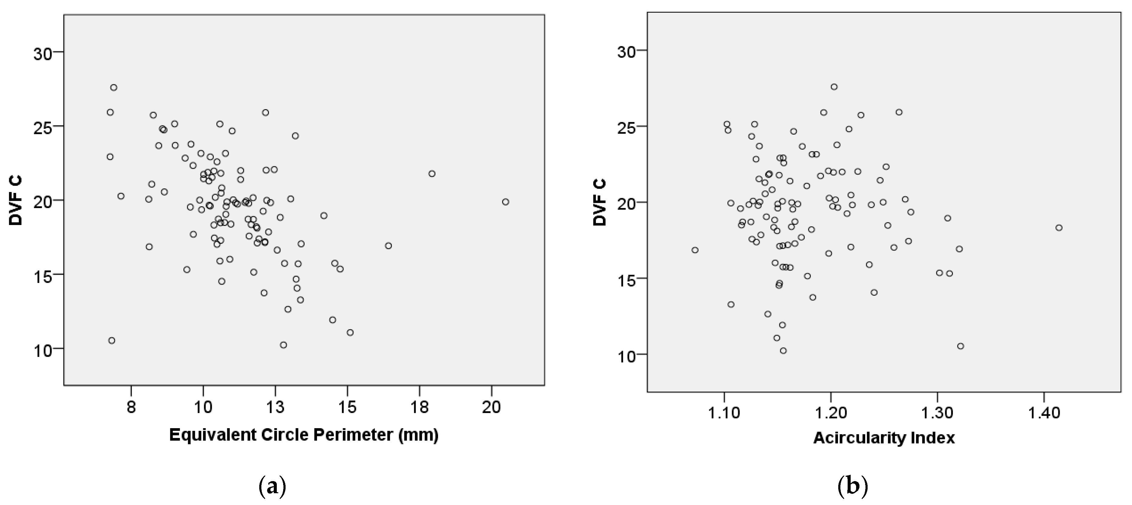
Figure 11 assesses the relationship between DVF C and equivalent circle perimeter ($P_2$) as well as between DVF C and acircularity index (A_index), using the Spearman correlation coefficient. Figure 11a suggests a steady relationship, with a moderate inverse correlation observed between DVF C and the equivalent circle perimeter (rs = –0.494, p ≤ 0.001). This indicates that the equivalent circle perimeter increases, while DVF C tends to decrease. Figure 11b shows that there is no statistically significant association between DVF C and the A_index.

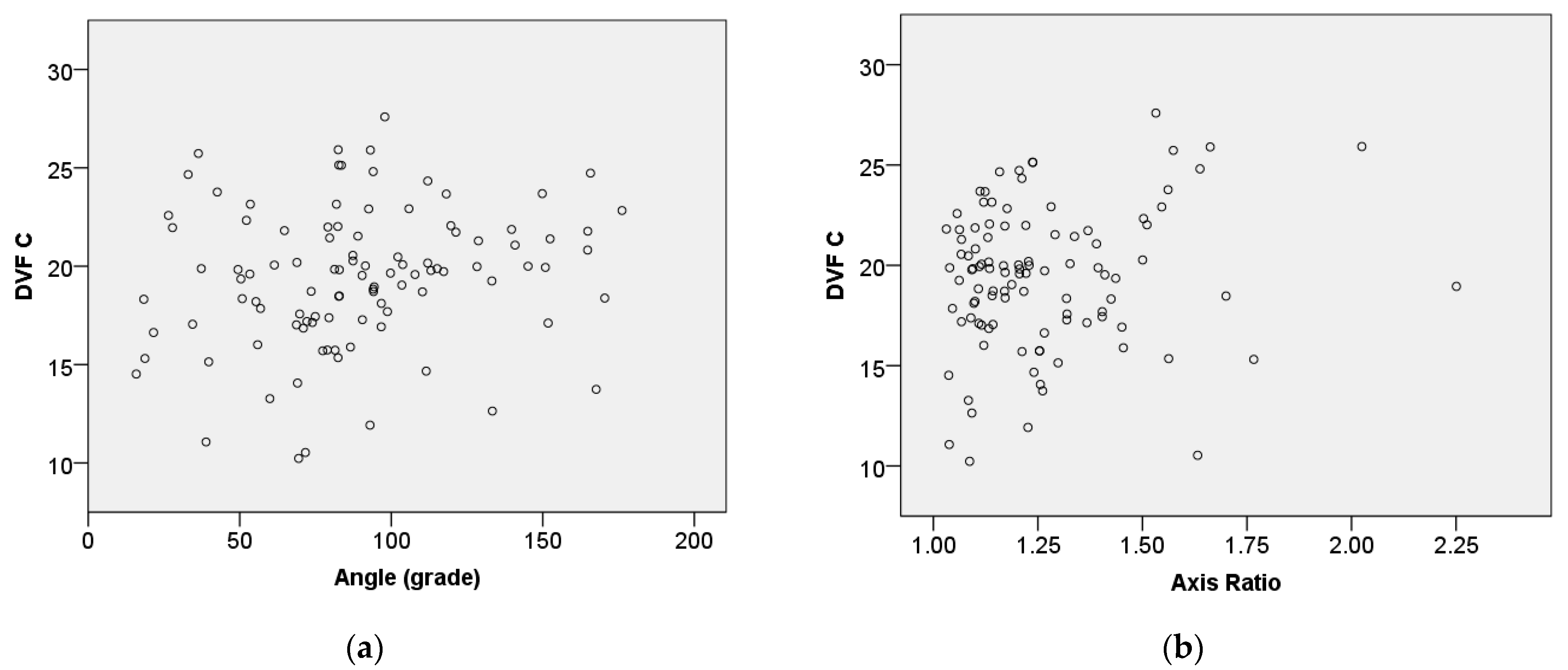
Figure 12 shows the relationship between central vascular density (DVF C) and angle (θ) as well as between axis ratio (A_ratio) and the Spearman correlation coefficient. Figure 12a suggests a consistent relationship, with a weak positive correlation observed between DVF C and the angle (rs = 0.232, p = 0.018). This indicates that as the angle increases, DVF C tends to increase slightly. Also, Figure 12b demonstrates that there is no statistically significant association between DVF C and the axis ratio.

The statistical analysis based on boxplot metrics offers a clear visual comparison of key data distribution between patient groups with type II diabetes and with both type II diabetes and high blood pressure. To identify significant differences in these parameters (e.g., medians across the groups), the Kruskal–Wallis H test is applied, highlighting FAZ metrics like perimeter and area as potential distinguishing factors between groups. Additionally, the Spearman rank correlation assesses the relationship between FAZ metrics and central vascular density, with significant correlations indicating strong relevance for distinguishing between patient groups.

Table 1. FAZ metric assessment across the three patient groups: control, type II DM, and type II DM + HBA.

Group	N	$\mathbf{Mean} {\mathit{P}}_1$	$\mathbf{Mean} {\mathit{A}}_1$	$\mathbf{Mean} {\mathit{P}}_2$	Mean A_index	Mean Angle (θ)	Mean A_ratio	Age
Control	6	9.74	5.86	8.48	1.15	110.35	1.39	>18
Type II DM	56	12.80	9.65	10.82	1.18	81.59	1.25	>18
Type II DM + HBP	41	14.08	11.65	11.93	1.17	95.42	1.24	>18

effectively highlights the differences in FAZ metrics among the three groups, suggesting that the presence of type II diabetes and hypertension impacts the size, shape, and orientation of the FAZ. Both the perimeter ($P_1$,) and area ($A_1$) of the FAZ increase from the control group to the type II DM group and further in the type II DM + HBP group. This suggests a trend of increasing FAZ size with the presence of type II diabetes and hypertension. Similarly, the equivalent circle perimeter ($P_2$) also shows an increasing trend from control to type II DM to type II DM + HBP groups. The acircularity index is slightly higher in the type II DM group (1.18) compared to the control (1.15) and type II DM + HBP (1.17) groups, indicating minor variations in the shape irregularity of the FAZ.

The mean angle of the FAZ decreases significantly in the type II DM group (81.59 degrees) compared to the control group (110.35 degrees) and partially recovers in the type II DM + HBP group (95.42 degrees). Also, the axis ratio is highest in the control group (1.39) and decreases in the type II DM (1.25) and type II DM + HBP (1.24) groups, indicating changes in the FAZ shape with disease progression.

These measurements are highly valuable for clinicians, as they provide the foundation for comprehensive statistical analysis, as shown in the Section 3.3.3.

The deep learning experiment was conducted using augmented images, a total of 672 cases, which included 42 images from healthy individuals, 357 images from type II diabetes (DM) patients, and 273 images from patients with both type II diabetes and high blood pressure (DM + HBP).

Augmentation techniques, such as rotation, scaling, and flipping, help simulate various imaging conditions and improve model robustness. This approach addresses potential overfitting and enables the model to generalize better across different scenarios, ultimately leading to improved accuracy in segmenting and analyzing FAZ metrics in the medical images under study.

The dataset was divided into an 80/20 split (80% for training and validation, and 20% for testing) to ensure that the model is trained on enough data while preserving an independent test set to assess its performance and generalizability.

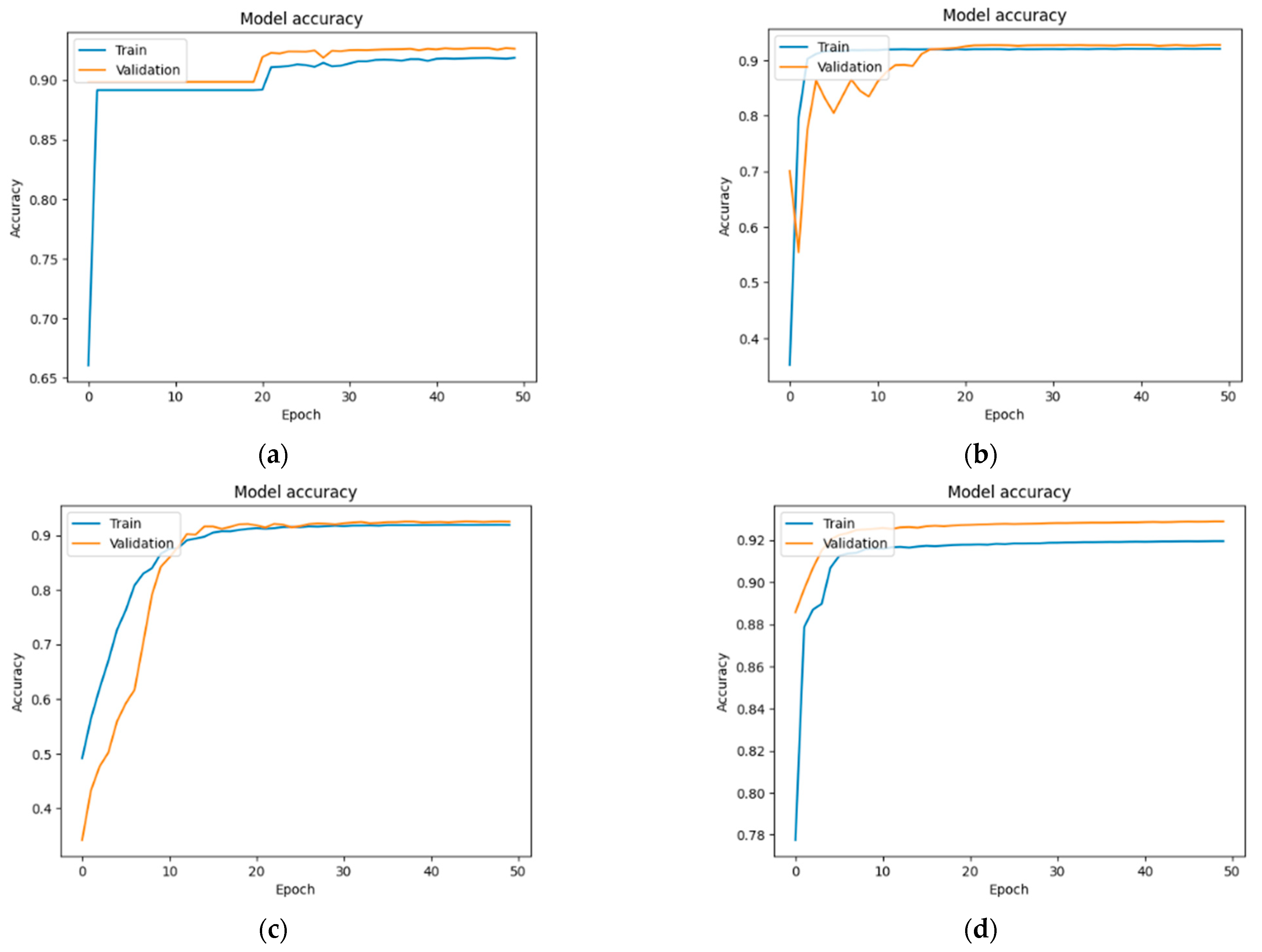
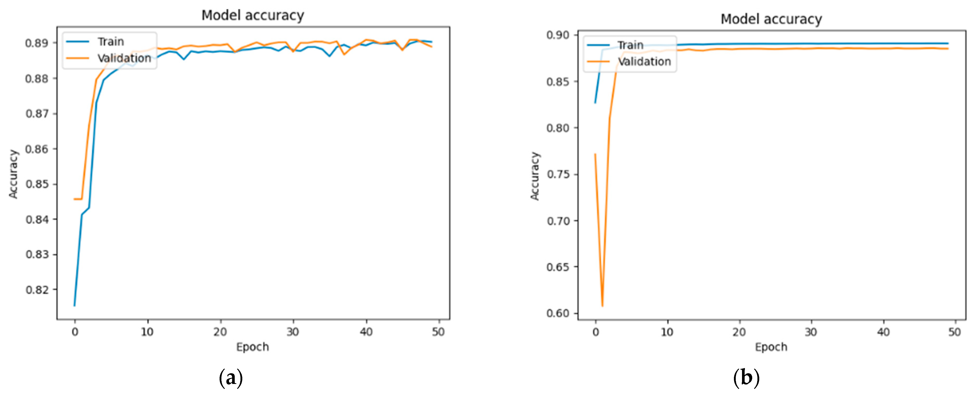
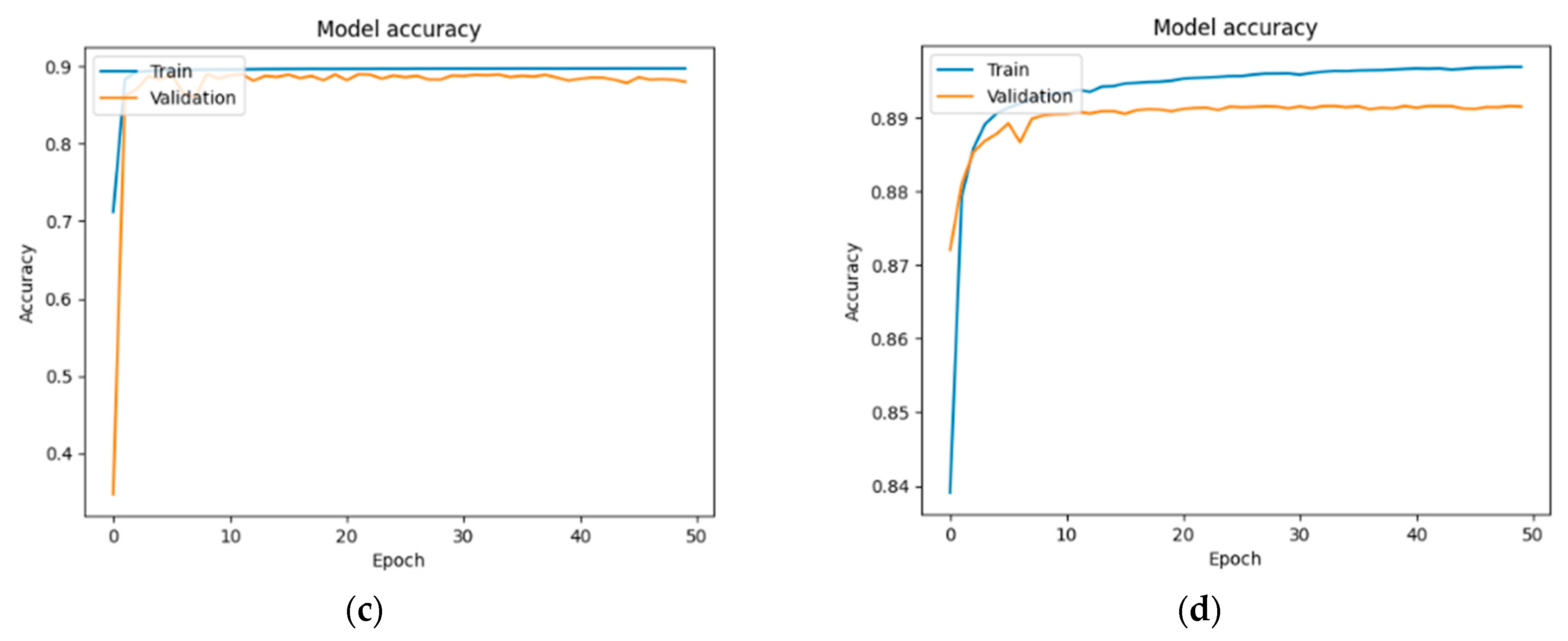
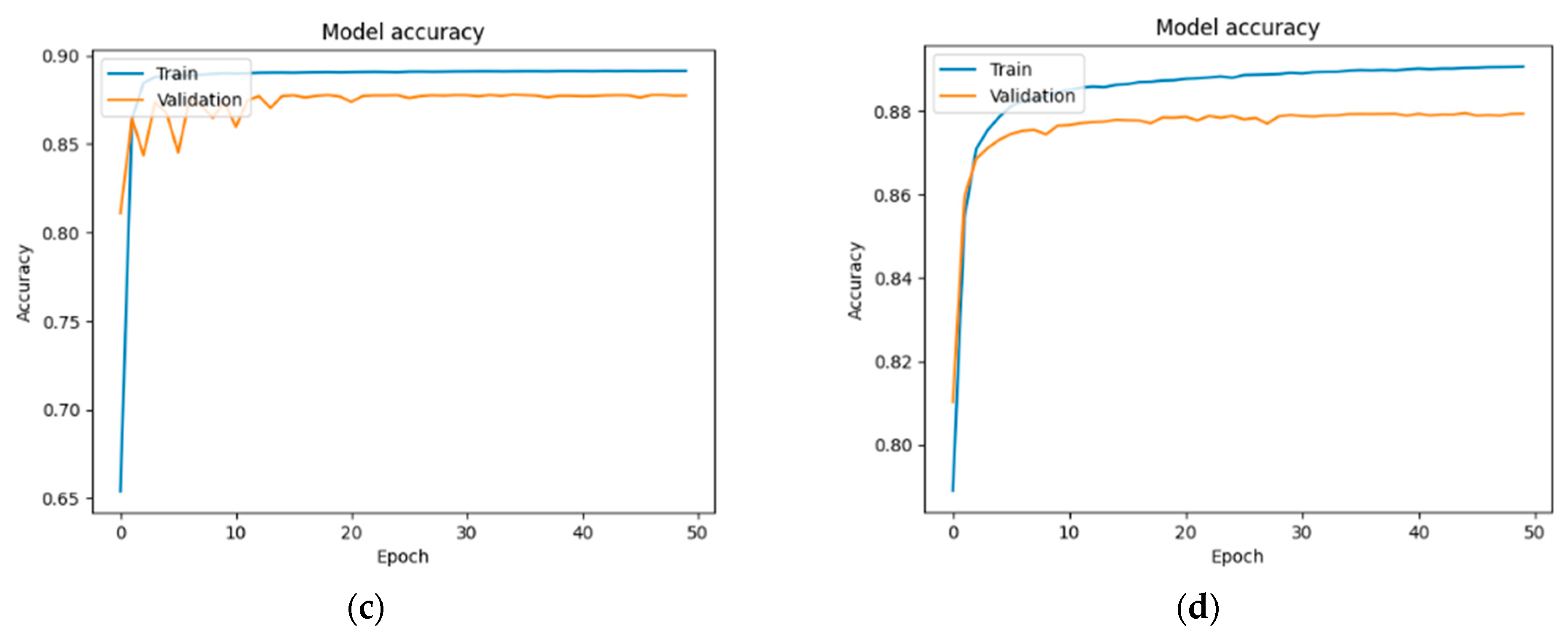
Figure 13, Figure 14 and Figure 15 show the training and validation accuracy for each group across different U-Net models. As detailed in the Section 3.4, the original 103 images were augmented and resized, resulting in a total of 672 images, each with a resolution of 224 × 224 pixels. The training and validation accuracies across different U-Net models show consistent performance with slight variations among the groups. In the case of the normal group (Figure 13), the values were as follows: 91.84% and 92.60%—U-Net; 92% and 92.69%—U-Net with DenseNet121; 91.90% and 92.50%—U-Net with MobileNetV2; and 91.09% and 91.54%—U-Net with VGG16.

In the case of the DM group (Figure 14): 89.02% and 88.88%—U-Net; 89.03% and 88.47%—U-Net with DenseNet121; 89.70% and 88.00%—U-Net with MobileNetV2; and 89.68% and 89.14%—U-Net with VGG16.

In the case of the DM + HBP group (Figure 15): 87.90% and 88.13%—U-Net; 88.87% and 89.05%—U-Net with DenseNet121; 89.12% and 87.73%—U-Net with MobileNetV2; and 89.06% and 87.93%—U-Net with VGG16.

Overall, while all models perform well, the choice of backbone architecture, DenseNet121, appears to have a slight impact on the model’s ability to generalize, particularly in more complex cases like the DM + HBP group.

The performance metrics obtained for each group across different U-Net models are presented in

Table 2. The evaluation results of the four DLs on the test dataset.

Model	Group	Accuracy [%]	IoU [%]	Dice Coefficient [%]
U-net	N	98.35	77.90	87.57
	Type II DM	96.32	73.02	84.40
	Type II DM + HBP	95.82	70.65	82.80
U-net + DenseNet121	N	98.73	82.50	90.41
	Type II DM	97.97	83.07	90.75
	Type II DM + HBP	97.46	80.09	88.94
U-net + MobileNetV2	N	98.48	78.40	87.89
	Type II DM	96.24	72.35	83.95
	Type II DM + HBP	96.93	76.56	86.72
U-Net + VGG16	N	98.00	72.82	84.27
	Type II DM	97.86	81.50	89.80
	Type II DM + HBP	97.27	79.03	88.28

.

The U-Net + DenseNet121 model outperforms the standard U-Net, U- Net + MobileNetV2 and U-Net + VGG16 models in terms of accuracy, IoU and Dice Coefficient, and this suggests that it is more robust for segmenting the FAZ area, particularly in patients with complex conditions like type II DM and HBP.

Also, all models show a drop in performance metrics (Accuracy, IoU, and Dice Coefficient) as the complexity of the conditions increases, from normal to type II DM and further to type II DM + HBP. The lower performance metrics in the type II DM + HBP group across all models indicate a potential challenge in segmenting more complicated pathological cases, highlighting areas for further model improvement or additional training with more diverse data.

5. Conclusions

This study presents two key contributions. First, it introduces a Python-based tool for extracting FAZ binary masks and determining FAZ metrics from full retina OCTA images, offering valuable clinical insights and enabling detailed statistical analysis of FAZ size and shape across three patient groups: healthy individuals, patients with type II diabetes mellitus, and those with type II diabetes mellitus and high blood pressure (HBP). Second, it evaluates four advanced deep learning models for segmenting the FAZ, particularly in complex pathological cases such as hypertension and type II diabetes mellitus, aiming to eliminate the need for manual segmentation and minimize the time demands on clinicians. The U-Net models integrated with DenseNet121 demonstrated promising results for FAZ segmentation, achieving a pixel accuracy of 97.46%, an IoU of 80.09%, and a Dice Coefficient of 88.94% in patients with both diabetes mellitus (DM) and hypertension. The results could be significantly enhanced with the collection of additional data, particularly because the current study represents a unique exploration of FAZ segmentation in full retina OCTA images for patients with both diabetes mellitus (DM) and hypertension. A larger dataset would provide the model with more diverse examples, helping it to better capture the variations in FAZ characteristics across different patient groups, particularly those with complex pathological conditions. Also, more data would allow for more comprehensive statistical analyses, offering deeper clinical insights and potentially uncovering new patterns or correlations related to FAZ size and shape in various patient populations.