Generating Mathematical Expressions for Estimation of Atomic Coordinates of Carbon Nanotubes Using Genetic Programming Symbolic Regression

Abstract

The study addresses the formidable challenge of calculating atomic coordinates for carbon nanotubes (CNTs) using density functional theory (DFT), a process that can endure for days. To tackle this issue, the research leverages the Genetic Programming Symbolic Regression (GPSR) method on a publicly available dataset. The primary aim is to assess if the resulting Mathematical Equations (MEs) from GPSR can accurately estimate calculated atomic coordinates obtained through DFT. Given the numerous hyperparameters in GPSR, a Random Hyperparameter Value Search (RHVS) method is devised to pinpoint the optimal combination of hyperparameter values, maximizing estimation accuracy. Two distinct approaches are considered. The first involves applying GPSR to estimate calculated coordinates ($u_c$, $v_c$, $w_c$) using all input variables (initial atomic coordinates u, v, w, and integers n, m specifying the chiral vector). The second approach applies GPSR to estimate each calculated atomic coordinate using integers n and m alongside the corresponding initial atomic coordinates. This results in the creation of six different dataset variations. The GPSR algorithm undergoes training via a 5-fold cross-validation process. The evaluation metrics include the coefficient of determination ($R^2$), mean absolute error ($MAE$), root mean squared error ($RMSE$), and the depth and length of generated MEs. The findings from this approach demonstrate that GPSR can effectively estimate CNT atomic coordinates with high accuracy, as indicated by an impressive $R^2\approx 1.0$. This study not only contributes to the advancement of accurate estimation techniques for atomic coordinates but also introduces a systematic approach for optimizing hyperparameters in GPSR, showcasing its potential for broader applications in materials science and computational chemistry.

1. Introduction

Carbon nanotubes (CNTs) are extraordinary nanoscale structures composed of carbon atoms arranged in a hexagonal lattice, forming cylindrical tubes [1]. They come in two main types: single-walled nanotubes (SWNTs), consisting of a single layer of carbon atoms, and multi-walled nanotubes (MWNTs), which comprise multiple concentric layers of graphene sheets. According to [2,3], the properties of CNTs are profoundly influenced by factors such as diameter, length, and chirality—the specific arrangement of hexagons in the lattice. CNTs are renowned for their exceptional mechanical strength [4], remarkable thermal conductivity [5], and outstanding electrical properties [6]. Due to these unique characteristics, they find applications across diverse fields, including materials science, electronics, and nanotechnology [7]. Their high strength-to-weight ratio makes them promising candidates for reinforcing materials [8], and their excellent electrical conductivity opens avenues for their use in nanoscale electronic devices [9]. Furthermore, CNTs hold potential in biomedical applications, such as drug delivery systems [10], owing to their nanoscale dimensions. The versatile properties of carbon nanotubes continue to fuel research and innovation in various scientific and technological domains.

The calculation of atomic coordinates for carbon nanotubes using density functional theory (DFT) involves defining the nanotube’s structural model, conducting geometry optimization through iterative adjustments of atomic coordinates to minimize total energy, and subsequently employing DFT for electronic structure calculations [11]. The total energy is evaluated based on the optimized atomic coordinates, providing insights into the nanotube’s stability. Visualization tools are then used to examine the optimized structure, and various properties such as bond lengths and electronic characteristics are analyzed. DFT calculations, commonly performed with software like VASP [12] or Quantum ESPRESSO [13], can be computationally intensive but yield crucial information about the nanotube’s atomic arrangement and properties at a fundamental level.

To the best of our knowledge, one paper was published in which artificial intelligence (AI) algorithms were used to estimate the calculated atomic coordinates of CNTs. In [14], the feed-forward neural network (FFNN), function fitting neural network (FITNET), cascade-forward neural network (CFNN), and generalized regression neural network (GRNN) have been used to estimate the calculated atomic coordinates obtained from DFT with high accuracy. To evaluate the estimation performance, the coefficient of determination ($R^2$), mean absolute error ($MAE$), and mean squared error ($MSE$) have been used. The results showed that the highest mean accuracy was achieved in the case of FITNET, i.e., $R^2=0.9999602$, $MAE=1.47\times {10}^{-3}$, and $MSE=6.625\times {10}^{-6}$, respectively. It should be noted that the dataset developed in [14] was also used in this research. The best results obtained in aforementioned research are listed in

Table 1. Results from other research.

Reference	AI-Algorithms	Estimation Perofrmance
[14]	FFNN	$R^2=0.99959$ $MAE=1.5365\times {10}^{-3}$ $RMSE=0.002584532$
	FITNET	$R^2=0.99996$ $MAE=1.47880\times {10}^{-3}$ $RMSE=0.002574049$
	CFNN	$R^2=0.99935$ $MAE=2.13075\times {10}^{-3}$ $RMSE=0.00328129$
	GRNN	$R^2=0.941247$ $MAE=0.22404$ $RMSE=0.279705$

.

The novelty and originality of this paper lie in its departure from the prevalent use of complex neural networks in prior research for estimating calculated atomic coordinates. While these networks deliver exceptional estimation accuracy, their drawback is the inability to transform the model into a straightforward mathematical form. This limitation impedes ease of use and demands substantial computational resources, including storage and CPU power, hindering the prediction of new atomic coordinates based on input variables.

In contrast, this paper introduces a groundbreaking approach by implementing a Genetic Programming Symbolic Regression (GPSR) algorithm on a dataset sourced from [14]. The key objective is to derive simple yet highly accurate Mathematical Expressions (MEs) capable of estimating atomic coordinates. This departure from complex neural networks is driven by the desire for a more interpretable and computationally efficient model.

To address the challenge of tuning numerous hyperparameters in GPSR, the paper introduces a Random Hyperparameter Value Search (RHVS) method. This innovative technique aims to pinpoint optimal GPSR hyperparameter values, facilitating the generation of MEs that achieve remarkable accuracy in estimating calculated atomic coordinates for CNTs. The proposed methodology is further strengthened by the application of the 5-fold cross-validation (5FCV) method during the GPSR training process, ensuring robustness and reliability in the model’s performance assessment.

In summary, this paper pioneers a novel approach by combining the interpretability of symbolic regression with the accuracy of GPSR, providing a solution to the limitations of previous research methods. The integration of RHVS for hyperparameter tuning adds a layer of sophistication, making this study a significant contribution to the field of computational chemistry and materials science.

Based on the previous research and the proposed idea, the following hypotheses are proposed:

• Is it possible to apply the GPSR algorithm on the publicly available dataset to obtain MEs that could estimate the calculated coordinates of CNTs with high estimation accuracy?
• Is it possible to develop and implement the RHVS method to find the optimal combination of GPSR hyperparameter values using which the MEs are obtained with high estimation accuracy?
• Is it possible to obtain a robust set of MEs and prevent overfitting by training of GPSR algorithm using the 5FCV training process?

This research is motivated by the limitations of using complex neural networks to estimate atomic coordinates, which lack interpretability and demand substantial computational resources. In contrast, we propose a novel approach utilizing the GPSR algorithm on a dataset from [14]. The aim is to generate simple yet highly accurate MEs for estimating atomic coordinates, addressing the shortcomings of previous methods. To optimize GPSR hyperparameters, we introduce the RHVS method. This innovative technique identifies optimal hyperparameter values, enhancing the accuracy of MEs in estimating CNTs’ atomic coordinates. The study’s novelty lies in combining the interpretability of symbolic regression with the accuracy of GPSR, offering a practical solution and contributing significantly to computational chemistry and materials science.

The presented research addresses problems associated with the limitations of previous methodologies, particularly the use of complex neural networks for estimating atomic coordinates. The drawbacks include high estimation accuracy but a lack of interpretability, impracticality in transforming models into simple mathematical forms, and significant computational resource requirements. The recent work becomes necessary to overcome these issues by introducing a shift from complex neural networks to a GPSR algorithm. This new approach aims to provide both high accuracy and simple, interpretable MEs, addressing the shortcomings of previous models. The incorporation of the RHVS method and the 5FCV process further enhances the accuracy and reliability of the proposed solution, making it a significant advancement in the field of computational chemistry and materials science.

The rest of the manuscript consists of the following sections, i.e., Materials and Methods, Results, Discussion, and finally, Conclusions. However, the best mathematical expressions are shown in Appendix A. The Materials and Methods section contains a description of the research methodology, dataset statistical analysis with outlier detection, a description of GPSR with the RHVS method, the training/testing process, and finally, the used computational resources. The Results section contains the results of a conducted investigation using which a discussion section is provided. Finally, in the Conclusions section, the conclusions are given based on the given hypotheses, advantages, and disadvantages of the proposed method with possible directions for future work. The additional Appendix A provides information about modifications to mathematical functions used in GPSR and a description of how to download and use the obtained MEs in this research.

2. Materials and Methods

The Materials and Methods section consists of Research Methodology, Dataset Description and Statistical Analysis, Genetic Programming Symbolic Regressor, Evaluation Metrics, and Training and Testing Procedure, respectively.

2.1. Research Methodology

The flow chart of the research methodology is shown in Figure 1.

As seen from Figure 1, the flowchart consists of the following steps:

• Dataset—Perform initial dataset analysis (correlation analysis, outliers analysis) to see if application of addition preprocessing techniques is required. After analysis, divide the dataset into train and test parts.
• Genetic Programming Symbolic Regressor—Application of Genetic Programming Symbolic Regressor method with random hyperparameter selection, and trained using 5-fold cross-validation process.
• Results—Application of evaluation metric methods on obtained MEs to determine which one of them has the highest classification performance and plotting the results.

2.2. Dataset Description and Statistical Analysis

To present this simple approach, a publicly available dataset from Kaggle [15] was utilized. The dataset consists of 8 variables and 10,721 samples. According to [14], the dataset was created by combining the atomic coordinates of elements and chiral vectors using the BIOVIA Materials Studio CASTEP software package.

The dataset variables are:

• chiral indices n—the parameter of the selected chiral vector;
• chiral indices m—the parameter of the selected chiral vector;
• initial atomic coordinate u—randomly generated parameter of the initial atomic coordinates of all carbon atoms;
• initial atomic coordinate v—randomly generated parameter of the initial atomic coordinate of all carbon atoms;
• initial atomic coordinate w—randomly generated parameters of the initial atomic coordinate of all carbon atoms;
• calculated atomic coordinates $u_c$;
• calculated atomic coordinates $v_c$;
• calculated atomic coordinates $w_c$.

The chiral indices (n and m) and initial atomic coordinates (u, v, and w) will be used as input dataset variables and the output target variables are calculated atomic coordinates ($u_c$, $v_c$, and $w_c$). The results of the statistical analysis of dataset variables are listed in

Table 2. The initial statistics of the carbon nanotube dataset.

	Count	Mean	Std	Min	Max
n	10,721	8.225725	2.138919	2	12
m		3.337189	1.683881	1	6
u		0.500064	0.286524	0.045149	0.954851
v		0.500072	0.286495	0.045149	0.954851
w		0.499637	0.288503	6.10 $\times {10}^{-5}$	0.999411
$u_c$		0.500064	0.290935	0.038504	0.961496
$v_c$		0.500072	0.291012	0.03893	0.96107
$w_c$		0.499834	0.289095	0	1

.

From Table 2, it can be noticed that all dataset variables do not have missing values. The variables n and m, when compared to the rest of the dataset variables, have higher mean, standard deviation, min, and max values. The initial atomic coordinates u and v and calculated atomic coordinates are almost similar when the results of statistical analysis are compared. The results of statistical analysis of initial and calculated atomic coordinates w and $w_c$ are also slightly different.

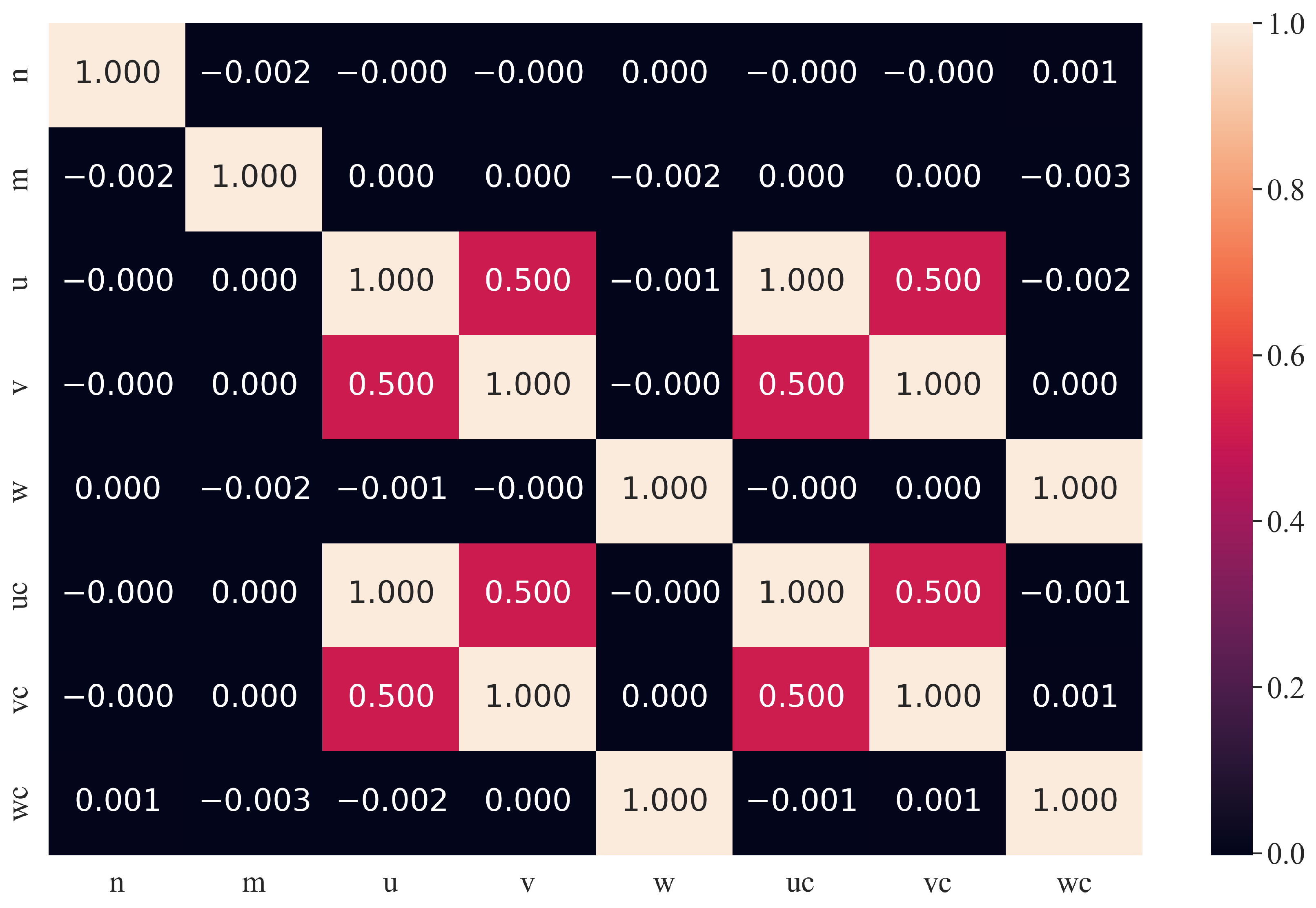
The correlation analysis was performed to determine if there is some correlation between input and output (targeted) variables in the dataset. Pearson’s correlation analysis [16] was performed, and the range of correlation values is from −1 to 1. A value of 0 is the worst correlation between two variables, i.e., the change in one variable value does not have any effect on the other variable. A value of −1 is the perfect negative correlation, and if the variable value decreases, the value of the other variable will increase and vice versa. A value of 1 is the perfect positive correlation, and if the one variable value increases, the value of the other variable will also increase.

The heatmap of the dataset is shown in Figure 2.

Figure 2 provides insights into the correlation structure within the dataset. Notably, the highest correlation value to the output variable $u_c$ is observed with the input variable u (correlation coefficient = 1.0). Furthermore, $u_c$ demonstrates a correlation of 0.5 with the variable v and near-zero correlations with the remaining input variables. Similar correlation patterns are observed for the output variable $v_c$, where v exhibits the highest correlation (correlation coefficient = 1.0), and a correlation of 0.5 is observed with u. Additionally, a correlation is noted between the initial atomic coordinates (u and v) and the calculated atomic coordinates ($u_c$ and $w_c$). A perfect correlation exists between w and $w_c$.

The final step involves scrutinizing the dataset for the presence of outliers, which are data points deviating significantly from the majority of the data [17]. Outliers, whether much higher or lower than typical values in the dataset, can exert a substantial impact on both statistical analyses and machine learning models. In machine learning, the presence of outliers can distort the learning process and compromise the model’s generalization ability.

Machine learning algorithms often rely on statistical measures and assumptions about the distribution of the data. Outliers, being atypical and aberrant, can distort these assumptions, leading to biased models or inaccurate predictions. Furthermore, outliers can disproportionately influence the determination of model parameters, leading to suboptimal results.

Detecting and addressing outliers is crucial for enhancing the robustness, accuracy, and reliability of machine learning models. It aids in producing more resilient models that perform well on unseen data by mitigating the impact of extreme values that might otherwise skew the learning process. Additionally, outlier detection serves as a quality control mechanism, helping to identify and rectify issues such as errors in data collection, measurement inaccuracies, or the presence of rare and impactful events. Overall, in the context of machine learning, outlier detection is an indispensable step in ensuring the integrity and effectiveness of the modeling process.

The boxplot for all dataset variables is shown in Figure 3.

Examining Figure 3, a comprehensive overview of the dataset’s distribution reveals that, for the most part, both input and output variables exhibit an absence of outliers. Nevertheless, a noteworthy observation is the presence of outliers in the input variable n. While the majority of data samples for n fall within the range of 3 to 12, there exist outliers below the lower threshold of 3. This deviation from the norm in the n variable prompts consideration of outlier treatment methods to ensure the robustness and reliability of subsequent analyses.

In addressing outliers, two common approaches are often considered: capping and trimming. Capping involves setting a threshold beyond which values are constrained, while trimming entails removing data points beyond a specified threshold. Given that the outliers in the variable n predominantly exhibit values below 3, the initial inclination was to apply capping or trimming as a corrective measure.

However, upon careful consideration, the decision was made to proceed with training the Genetic Programming Symbolic Regression (GPSR) algorithm using the original dataset, including the outliers. This decision stems from an appreciation of the potential information embedded in these outlier values, which may contribute to the model’s capacity to capture diverse patterns and nuances within the data.

It is recognized that outright removal of outliers, especially when they represent valid and meaningful variations in the dataset, may lead to a loss of valuable insights. The chosen approach aligns with the intention to leverage the entirety of the dataset, even with the presence of outliers in the variable n, in order to enable the GPSR algorithm to discern and incorporate the full spectrum of patterns and relationships within the data.

The problem with GPSR is that the algorithm must be trained for each calculated value of atomic coordinates. The idea was also to investigate the number of input variables required to estimate the calculated atomic coordinates. The list of considered cases is shown in

Table 3. The dataset variations on which GPSR was applied with GPSR variable representation.

Case	Input Variables					Output Variable
$nmuvw$-$u_c$	n	m	u	v	w	$u_c$
Variables represented in GPSR	$X_0$	$X_1$	$X_2$	$X_3$	$X_4$	$y_{u_c}$
$nmuvw$-$v_c$	n	m	u	v	w	$v_c$
Variables represented in GPSR	$X_0$	$X_1$	$X_2$	$X_3$	$X_4$	$y_{v_c}$
$nmuvw$-$w_c$	n	m	u	v	w	$w_c$
Variables represented in GPSR	$X_0$	$X_1$	$X_2$	$X_3$	$X_4$	$y_{u_c}$
$nmu$-$u_c$	n	m	u	/	/	$u_c$
Variables represented in GPSR	$X_0$	$X_1$	$X_2$	/	/	$y_{u_c}$
$nmv$-$v_c$	n	m	v	/	/	$v_c$
Variables represented in GPSR	$X_0$	$X_1$	$X_2$	/	/	$y_{v_c}$
$nmw$-$w_c$	n	m	w	/	/	$w_c$
Variables represented in GPSR	$X_0$	$X_1$	$X_2$	/	/	$y_{w_c}$

.

From Table 3, it can be noticed there are 6 different dataset variations derived from the original one on which the GPSR algorithm will be applied to obtain MEs that can estimate the corresponding calculated atomic coordinates with high accuracy.

2.3. Genetic Programming Symbolic Regression

Genetic Programming Symbolic Regression (GPSR) is an evolutionary algorithm [18] that begins the execution by building an initial population that is unfit for a particular task. However, through the application of genetic operators through a pre-defined number of generations, in the end, the best solution for the population is obtained that is fitted for a particular task as much as possible.

To create an initial population, several hyperparameters have to be defined, i.e., the size of the initial population (Size_Pop), the range of constant values (cnst_vals), the set of mathematical functions (Set_fun), and the method used for the creation of the initial population (meth_init). The Set_fun used in this research consists of +, −, *, /, √, log, ∛, ${log}_2$, ${log}_{10}$, sin, cos, tan, and $\left|\right|$. The /, √, log, ${log}_2$, and ${log}_{10}$ had to be modified to avoid the occurrence of imaginary or non-number values. These functions are defined in Appendix A.1. The input variables and the target variable are defined by GPSR when the dataset is imported.

The size of the initial population and the population that will be evolved during the GPSR execution is defined with the Size_Pop hyperparameter value. To develop each member of the initial population, the input variables, constant values from cnst_vals range, and mathematical functions from Set_fun are randomly chosen. It should be noted that population members in GPSR are represented as tree structures, which means that their size is defined by the depth starting from the root node. In all investigations conducted in this paper using the GPSR algorithm on the initial population, the ramped half-and-half method [19] was used. Using this method, 50% of the initial population is created using full, while the other half uses the grow method. The term ramped refers to a defined depth of symbolic expressions that are defined in a certain range. The initial depth (init_depth) hyperparameter value defines the depth range used for the creation of the initial population.

When the initial population is created, the population members have to be evaluated to calculate the fitness function value, i.e., determine the quality of each population member. First, the input variable values are provided to each ME to calculate the output and then this calculated output is compared to real output to obtain the fitness function value. The fitness function used in all these investigations is a mean absolute error ($MAE$) [20] and can be calculated using the following expression:

$$MAE=\frac{{\sum }_{i=1}^n|y_{ti}-y_{pi}|}{n},$$

(1)

where $y_{ti}$ is the true target value (dataset target value), and $y_{pi}$ is the predicted value obtained from ME. The n is the number of dataset samples.

After the population is evaluated, some population members have to be chosen to be parents of the next generation. On these parents, genetic operations will be performed to produce offspring for the next generation. In this investigation, the tournament selection method is used where population members are randomly chosen and they compete against each other. The best population member then becomes the winner of the tournament selection (parent), and on the winner, genetic operations are performed. The size of the tournament selection is defined with hyperparameter value t_size.

In GPSR, four different genetic operations were used, i.e., crossover, point mutation, hoist mutation, and subtree mutation. The sum of all genetic operations should be near 1 to reduce the reproduction of population members, i.e., to reduce the number of population members that enter the next generation unchanged. To perform all three mutations, only one tournament selection winner is required. In the case of point mutation, the random nodes are chosen on the tournament winner. The constants are replaced with randomly chosen constants, variables with other variables, and functions with other functions. However, in the case of functions, the arity between old and new functions must be the same. In the case of hoist mutation, the subtree is randomly selected, and on that subtree, a random node is selected which replaces the entire subtree. The subtree mutation randomly chooses a subtree that is replaced with a randomly generated subtree. The crossover operation requires two tournament selection winners and a random subtree is selected from the first winner and is replaced with a randomly selected subtree of the second winner.

The GPSR, like other types of evolutionary algorithms, can execute indefinitely without the application of termination criteria. In GPSR, two hyperparameters can be used to terminate its execution and these are the stopping criteria value (crit_stop) and the maximum number of generations (max_gen). The stopping criteria value is the predefined minimum value of the fitness function, and if the value is reached by one of the population members during GPSR execution, the GPSR execution will be terminated. On the other hand, the maximum number of generations is the predefined number of generations through which GPSR population members will evolve. After that predefined number is reached, the GPSR execution will be terminated. In all these investigations the GPSR algorithm was terminated after a maximum number of generations was reached.

The maximum number of samples (max_samp) hyperparameter value specifies the size of randomly selected samples from the training dataset that will be used to evaluate population members.

During the GPSR execution, the size of the population members can rapidly grow without any benefit to the fitness value. This phenomenon is called the bloat phenomenon, and to prevent its occurrence, the parsimony pressure method was utilized. This method requires the definition of the parsimony coefficient (CO-Pars) hyperparameter value. This coefficient is used during the tournament selection where the fitness value of large programs is modified with the parsimony coefficient using the expression:

$$f_p\left(x\right)=f\left(x\right)+cl\left(x\right),$$

(2)

where $f_p$, f, c, and l are modified fitness function values, original fitness function value, parsimony coefficient, and population member size, respectively. So, the parsimony coefficient is multiplied by the population member size and added to the original fitness function value. With the application of the parsimony pressure method, the fitness value of large population members increases, which makes them less favorable for selection in the tournament selection method. The population member size can be measured as depth or length; however, in this case, the member size is length. The problem with this coefficient is that this coefficient is the most sensitive one. Large values can prevent the growth of population members, while small values can rapidly lead to a bloat phenomenon.

To develop the RHVS method for GPSR hyperparameter selection, first, the lower and upper boundaries of each hyperparameter are defined. Each of these boundaries is initially tested, and if necessary, adjusted before performing training on GPSR using 5FCV. The list of GPSR hyperparameters with lower and upper boundaries is shown in

Table 4. The list of RHVS boundaries for random selection of GPSR hyperparameters.

Hyperparameter Name	Lower Boundary	Upper Boundary
Size_Pop	1000	2000
cnst_vals	−10,000	10,000
init_depth	3	15
t_size	100	500
crossover	0.001	1
point mutation	0.001	1
hoist mutation	0.001	1
subtree mutation	0.001	1
crit_stop	0	$1\times {10}^{-6}$
max_gen	300	500
max_samp	0.99	1
CO-Pars	0	$1\times {10}^{-3}$

.

Two hyperparameters were left out of Table 4, i.e., meth_init and Set_fun. The meth_init used in this research is previously described as random half-and-half. All previously defined mathematical functions were available to the Set_fun hyperparameter, from which the GPSR algorithm randomly selected mathematical functions to create the initial population and later for application of genetic operators.

2.4. Evaluation Metrics

To determine the quality of the obtained MEs, the size (depth and length), coefficient of determination ($R^2$), mean absolute error ($MAE$), and root mean squared error ($RMSE$) were used.

As described earlier, the population member inside GPSR is measured in terms of length and depth. The depth is the size of the mathematical equation represented in tree form, while the length is the length of ME. The coefficient of determination ($R^2$) [21] can be described as the ratio of the variation in the predictable dependent variable from the independent variable. The formula for calculating the $R^2$ can be written as:

$$R^2=1-\frac{S{S}_{res}}{S{S}_{tot}}=1-\frac{{\sum }_i{(y_i-f_i)}^2}{{\sum }_i{(y_i-\overline{y})}^2},$$

(3)

where y is the output vector, and $\overline{y}$ is the mean value of the observed data.

The expression for calculating the $MAE$ value [20] is given in the previous subsection, since it is also used as the fitness function in the GPSR algorithm. The $RMSE$ is used to measure the difference between predicted values obtained from the model/estimator and the real (dataset) target values. The $RMSE$ value [20] can be obtained using the expression:

$$RMSE=\sqrt{\frac{{\sum }_{i=1}^N|y_i-{\hat{y}}_i|}{N}}.$$

(4)

where N is the total number of samples, $y_i$ is the dataset target value, and ${\hat{y}}_i$ is the predicted value made by the trained model/estimator.

2.5. Training and Testing Process

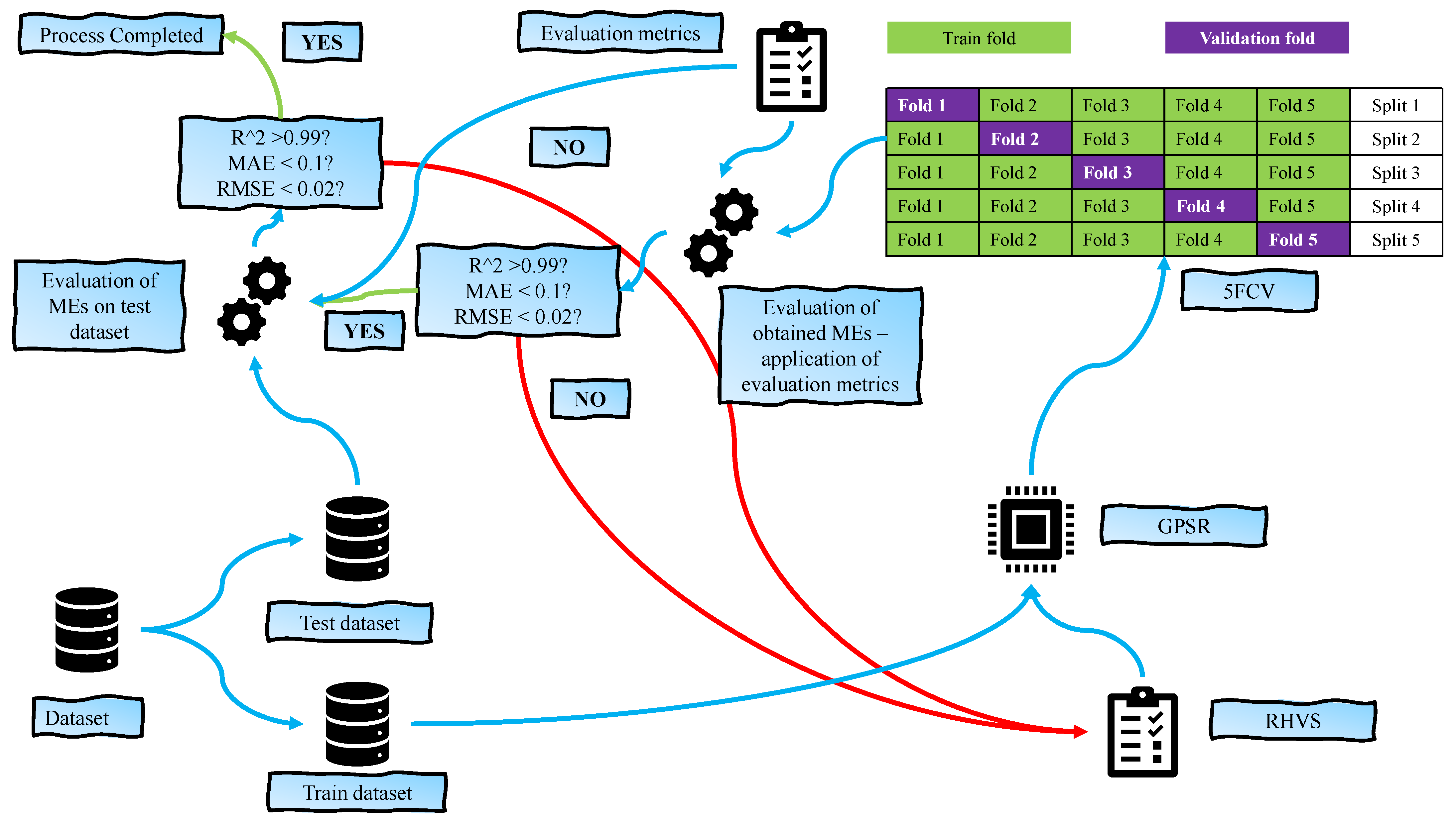
The graphical representation of the training and testing process is shown in Figure 4.

As seen from Figure 4, the dataset underwent an initial division into training and testing datasets, following a standard 70:30 ratio. This division strategy ensures a sufficiently large training set for model development, while reserving a distinct portion for assessing the model’s performance on unseen data. The training dataset played a pivotal role in the training of the Genetic Programming Symbolic Regression (GPSR) algorithm, employing the 5-Fold Cross-Validation (5FCV) method.

The training procedure aligns with the methodology employed in [22], ensuring a consistent and validated approach. After the 5FCV process, the resulting set of Mathematical Expressions (MEs) is subjected to evaluation, primarily focusing on estimating accuracy on the training dataset. The assessment criteria involve scrutinizing metrics such as the coefficient of determination ($R^2$), mean absolute error ($MAE$), and root mean squared error ($RMSE$). The desired benchmark for successful training is set ambitiously high, aiming for $R^2>0.99$, $MAE<0.1$, and $RMSE<0.02$.

Should the estimation accuracy not meet these stringent criteria, the process initiates anew with the selection of random hyperparameter values. This iterative approach aims to systematically explore hyperparameter space and fine-tune the model for optimal performance.

Conversely, if the obtained set of MEs satisfies the defined criteria, the model proceeds to the testing phase. The MEs are then evaluated on the reserved 30% of the dataset designated for testing. The evaluation metrics—$R^2$, $MAE$, and $RMSE$—are computed to gauge the model’s generalization performance on unseen data.

Should the evaluation metrics on the test dataset fail to meet the set criteria, indicating potential overfitting, the process reverts to the beginning, invoking the Random Hyperparameter Value Search (RHVS) method for refining the model. Conversely, if the evaluation metrics on the test dataset align with the predefined criteria, signifying robust generalization, the training and testing process is deemed complete. This meticulous procedure ensures the development of a GPSR model that not only excels in training but also demonstrates high performance on new and unseen data.

3. Results

At the end of the subsection entitled Dataset Description and Statistical Analysis, it was stated that six different cases were considered. Here, the results are presented in two subsections, i.e., first three cases with all dataset inputs to obtain MEs for estimation of $u_c$, $v_c$, and $w_c$, and the other three cases in which selected input variables are used to obtain MEs for estimation of $u_c$, $v_c$, and $w_c$. Due to the large number of MEs and their size, the MEs will not be shown in the paper. However, they can be downloaded from the GitHub repository (link available in Appendix A.2).

3.1. All Input Variables

Here, the results of three different GPSR algorithms, trained using 5FCV to obtain MEs that can estimate $u_c$, $v_c$, and $w_c$ with high accuracy, are presented. The optimal GPSR hyperparameter values obtained using the RHVS method are shown in

Table 5. The optimal GPSR hyperparameter values are chosen by the RHVS method, using which the best set of MEs are obtained on each dataset variation.

Case	GPSR Hyperparameter Values (Size_Pop, Max_Gen, t_Size, Init_Depth Crossover, Subtree Mutation, Hoist Mutation, Point Mutation, Crit_Stop, Max_Samp, CO-Pars)
$nmuvw$-$u_c$	1166, 380, 366, (3, 9), 0.021, 0.953, 0.02, 0.0039, $6.22\times {10}^{-7}$, 0.99, (−2929.06, 8732.5), 0.00086
$nmuvw$-$v_c$	1580, 465, 419, (7, 8), 0.032, 0.96, 0.0042, 0.0021, $2.49\times {10}^{-7}$, 0.99, (−2239.26, 5430.02), $2.98\times {10}^{-5}$
$nmuvw$-$w_c$	1658, 481, 249, (3, 15), 0.027, 0.95, 0.0054, 0.012, $5.18\times {10}^{-7}$, 0.99, (−4451.28, 2031.56), 0.00043

.

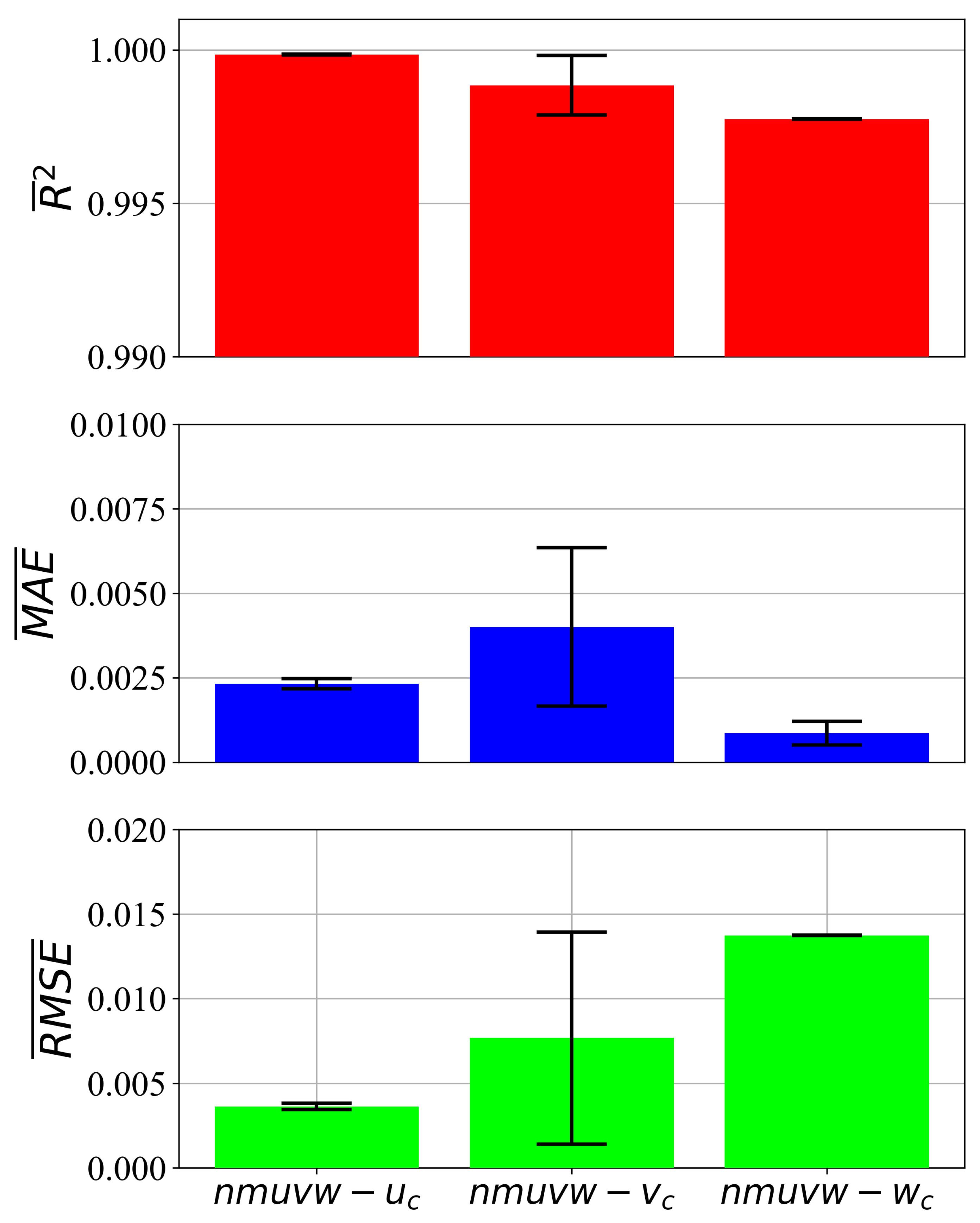
From Table 5, it can be noticed that the lowest size of the population was used in the case of $nmuvw$-$u_c$. The most dominating genetic operator in all three cases was subtree mutation, with a value of 0.95 or higher. The crit_stop value was extremely low in all cases and was never reached during GPSR execution. The CO-Pars value was the lowest in the case of $nmuvw$-$v_c$. In Figure 5, the estimation performance of the best MEs is shown.

Analyzing the results depicted in Figure 5 reveals intriguing insights into the estimation performance across different cases. Notably, the highest mean value of $R^2$ and the lowest values of $MAE$ and $RMSE$ are observed in the case of $nmuvw$-$u_c$. This signifies a superior level of accuracy and precision in the estimation of the calculated atomic coordinates, reflecting the efficacy of the GPSR algorithm in capturing the underlying patterns in the dataset.

In the second case, $nmuvw$-$v_c$, a slightly lower $R^2$ is observed, leading to marginally higher $MAE$ and $RMSE$ values compared to the $nmuvw$-$u_c$ case. However, it is crucial to note the presence of larger error bars ($\sigma$ values), indicating a higher variability in the estimation performance. This suggests that while, on average, the estimation performance is slightly lower than in the first case, there is greater variability in individual predictions.

The third case, $nmuvw$-$w_c$, exhibits the lowest $R^2$ and $MAE$ values, with $RMSE$ being the highest among the three cases. However, an interesting observation is the absence of $\sigma$ values in the case of $R^2$ and $RMSE$. This implies a more consistent and less variable performance in terms of coefficient of determination and root mean squared error compared to the $nmuvw$-$v_c$ case. Despite the lower mean values in accuracy metrics, this case demonstrates a more stable and predictable estimation performance.

The nuanced differences observed across these cases highlight the intricacies in estimating different atomic coordinates using the GPSR algorithm. The trade-off between mean performance and variability, as evidenced by the presence of error bars, underscores the need for a nuanced evaluation of the algorithm’s effectiveness across distinct output variables. This thorough analysis enhances our understanding of the algorithm’s strengths and limitations, providing valuable insights for refining and optimizing future implementations. The depth, length, mean depth, and mean length values of obtained MEs are listed in

Table 6. The depth and length of obtained MEs in cases where all input variables were used.

Dataset Type	Depth	Length	Mean Depth	Mean Length
$nmuvw$-$u_c$	16/28/17/19/21	64/142/58/36/72	20.2	74.5
$nmuvw$-$v_c$	38/41/34/34/31	285/517/224/250/186	35.6	292.4
$nmuvw$-$w_c$	19/7/13/10/17	212/18/30/16/51	13.2	65.4

.

By comparing the depth and length values of obtained MEs for all three cases listed in Table 6, it can be noticed that the MEs with the lowest depth and length were obtained in the case of $nmuvw$-$w_c$. The largest MEs were obtained in the case of $nmuvw$-$v_c$. It is also interesting to notice that for the same values of depth (third and fourth ME in the case of $nmuvw$-$v_c$, equaling 34), the obtained MEs have different length values, i.e., 224 and 250, respectively.

3.2. Selected Input Variables

In this subsection, the results of the application of GPSR on the remaining three dataset variations are shown ($nmu$-$u_c$, $nmu$-$v_c$, and $nmu$-$w_c$) to obtain MEs for estimation of $u_c$, $v_c$, and $w_c$. In

Table 7. The optimal hyperparameter values found using RHVS method.

Case	GPSR Hyperparameter Values (Size_Pop, Max_Gen, t_Size, Init_Depth Crossover, Subtree Mutation, Hoist Mutation, Point Mutation, Crit_Stop, Max_Samp, CO-Pars)
$nmu$-$u_c$	1091, 492, 483, (7, 13), 0.01, 0.97, 0.0022, 0.013, $7.018\times {10}^{-8}$, 0.99, (−6987.98, 9366.61), 0.00052
$nmv$-$v_c$	1762, 455, 234, (6, 9), 0.0022, 0.966, 0.01168, 0.018, $5.309\times {10}^{-7}$, 0.995, (−7321.94, 8132.74), 0.00038
$nmw$-$w_c$	1455, 383, 124, (3, 13), 0.0017, 0.95, 0.024, 0.02, $9.39\times {10}^{-8}$, 0.996, (−7726.074, 3767.204), 0.00031

, the optimal hyperparameters obtained using the RHVS method, using which GPSR generated MEs with high estimation accuracy, are shown.

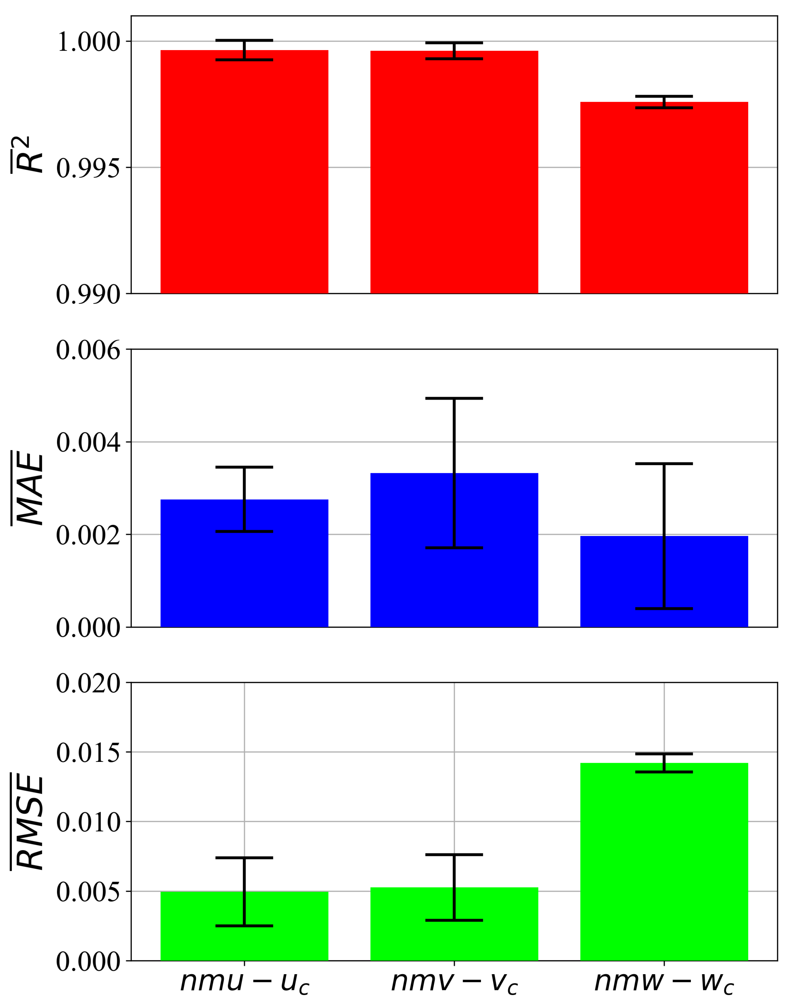
As seen from Table 7, the smallest population size (1091) was used in the case of $nmu$-$u_c$; however, the evolution of this population was the longest (492 generations). Again, the subtree mutation was the dominating genetic operation in all three cases, with values of 0.95 or higher. As in the previous three cases, the crit_stop (smallest fitness function value) was never reached due to its extremely low value. The CO-Pars (parsimony coefficient) value was the smallest in the $nmw$-$w_c$ case. The evaluation metric values for all three cases are graphically shown in Figure 6.

Examining the outcomes presented in Figure 6 provides an in-depth understanding of the estimation performance across various scenarios. Notably, the highest mean $R^2$ value is achieved in the case of $nmu$-$u_c$, indicating an exceptional level of goodness of fit for this particular atomic coordinate estimation. Following closely is the case of $nmv$-$v_c$, which exhibits a slightly lower mean $R^2$ but still attains a commendable level of explanatory power. The case of $nmw$-$w_c$ follows suit, with the lowest mean $R^2$ among the three scenarios. This hierarchy of mean $R^2$ values sheds light on the algorithm’s ability to capture and explain the variance in the dataset, emphasizing its proficiency in certain estimation scenarios.

In terms of mean $MAE$ values, the case of $nmw$-$w_c$ emerges as the most accurate, reflecting the smallest average absolute errors in atomic coordinate estimation. This suggests that, on average, the GPSR algorithm demonstrates superior accuracy in predicting the calculated atomic coordinates for $nmw$-$w_c$. It is noteworthy that the other cases, $nmu$-$u_c$ and $nmv$-$v_c$, while having larger mean $MAE$ values, still maintain reasonably low levels of absolute error.

However, the examination of standard deviation ($\sigma$) values unveils interesting nuances. In the cases of $nmv$-$v_c$ and $nmw$-$w_c$, despite their higher mean $MAE$ values, larger $\sigma$ values indicate greater variability in the estimation errors. This implies that, while these cases might exhibit higher mean errors on average, there is also a broader range of errors, suggesting a more varied performance across different instances. Contrastingly, in the case of $nmu$-$u_c$, despite having a larger mean $MAE$, the $\sigma$ value is comparatively smaller, suggesting a more consistent and predictable estimation performance.

Considering the mean $RMSE$ values, the case of $nmu$-$u_c$ stands out, with the smallest average root mean squared errors. This signifies a superior overall precision in this particular atomic coordinate estimation scenario. However, it is essential to note that, similar to $MAE$, the $\sigma$ values for $RMSE$ are relatively larger in the cases of $nmu$-$u_c$ and $nmv$-$v_c$, indicating a broader range of errors.

This detailed exploration of mean and variability metrics across different atomic coordinate estimation scenarios underscores the nuanced performance of the GPSR algorithm. It provides valuable insights into the algorithm’s strengths and weaknesses, aiding in the identification of optimal scenarios for its application and guiding future refinements for enhanced accuracy and stability. The depth and length of obtained MEs are listed in

Table 8. The depth and length of obtained MEs.

Dataset Type	Depth	Length	Mean Depth	Mean Length
$nmu$-$u_c$	20/28/28/20/22	137/335/68/113/168	23.6	164.2
$nmv$-$v_c$	38/30/20/22/19	333/458/160/157/133	25.8	248.2
$nmw$-$w_c$	3/36/19/24/21	11/123/62/181/61	20.5	87.6

.

From Table 8, it can be noticed based on mean depth and mean length values that the smallest MEs were obtained for the estimation of $w_c$ CNT coordinates. However, the largest MEs were obtained in the case of $v_c$ estimation. From Table 8, it can be noticed that for the same values of depth, the length of MEs is quite different. This is especially evident in the case of MEs obtained for estimation of $u_c$, where the depth of the second and third MEs is the same (28), while the length of MEs is 335 and 68. This difference in length can be attributed to the number of mathematical functions used to obtain these MEs. The second equation has a large number of mathematical functions, while the third uses more constants and input variables. Further analysis of MEs showed that a potential bloat phenomenon occurred during GPSR on different 5FCV splits. In the case of the second ME, the size of population members in GPSR execution grew rapidly to lower the fitness function value, while in the case of the third ME, the fitness function was constantly lowered from generation to generation, without a significant increase in the population member size.

Unfortunately, the analysis of required input variables in obtained MEs showed that all input variables used in dataset variation are required to calculate the corresponding output.

4. Discussion

The utilization of a publicly available dataset in this research unveils intriguing characteristics, notably a generally low correlation between variables. The highest correlation of 1 is observed between input atomic coordinates and the corresponding calculated coordinates. Additional correlations of 0.5 exist between $u-v$, $u-v_c$, and $v-u_c$. Interestingly, the dataset exhibits outliers in only the input variable n, a phenomenon typically expected to influence the performance of AI algorithms. However, in this investigation, the presence of outliers did not adversely affect algorithm performance.

To delve into the intricacies of the dataset, six variations were created, as outlined in Table 3. Three variations aimed to estimate the calculated values of $u_c$, $v_c$, and $w_c$, while the other three selected input variables to estimate the corresponding calculated coordinates ($u_c$, $v_c$, and $w_c$).

The implementation of the Genetic Programming Symbolic Regression (GPSR) algorithm, coupled with the Random Hyperparameter Value Search (RHVS) and 5-Fold Cross-Validation (5FCV) methods, provided a robust framework for model training. The application of GPSR on all six dataset variations resulted in the generation of 30 best Mathematical Expressions (MEs), with 5 MEs obtained for each dataset variation through 5FCV.

The optimal hyperparameters, derived using RHVS for the first three dataset variations ($nmuvw$-$u_c$, $nmuvw$-$v_c$, and $nmuvw$-$w_c$), are detailed in Table 5. Notably, variations in hyperparameters reflect distinct characteristics of each estimation scenario. For instance, the smallest population size is used in the case of $nmuvw$-$u_c$, while the $nmuvw$-$w_c$ scenario involves the longest execution due to a larger max_gen value. These insights shed light on the intricate interplay between hyperparameter selection and estimation scenario complexity.

Comparing Table 5 and Table 7, the dominance of subtree mutation as a genetic operation is evident. The low crit_stop values suggest that stopping criteria were not met by any population member during GPSR executions, leading to termination after reaching max_gen. Additionally, the parsimony coefficient (CO-Pars) mainly influenced cases where $nmuvw$-$v_c$ and $nmv$-$v_c$ produced the largest MEs in terms of length.

Moving to the performance evaluation metrics, Figure 5 and Figure 6 offer valuable insights. The highest mean $R^2$ values are consistently achieved when $u_c$ is the target variable, whereas the lowest mean $R^2$ values are observed when $w_c$ is the target. Surprisingly, in the case of $w_c$ as the output variable, despite having the lowest $R^2$ and the highest $RMSE$, the $MAE$ value is the second-best, indicating a nuanced performance.

An examination of the depth and length of MEs (Table 6 and Table 8) unveils a trend where larger MEs are obtained when output variables are estimated with fewer input variables. This observation is attributed to the scarcity of input variables correlated with the output variable.

In conclusion, this comprehensive analysis offers a deep understanding of the dataset characteristics, the interplay of hyperparameters, and the nuanced performance of the GPSR algorithm across different estimation scenarios. These findings contribute valuable insights for refining the algorithm, guiding future implementations, and advancing the understanding of symbolic regression in the context of atomic coordinate estimation.

The best results obtained in this research are compared to the results from the literature described in the Introduction section and shown in

Table 9. Comparison of the results.

Reference	AI-Algorithms	Estimation Perofrmance
[14]	FFNN	$R^2=0.99959$ $MAE=1.5365\times {10}^{-3}$ $RMSE=0.002584532$
	FITNET	$R^2=0.99996$ $MAE=1.47880\times {10}^{-3}$ $RMSE=0.002574049$
	CFNN	$R^2=0.99935$ $MAE=2.13075\times {10}^{-3}$ $RMSE=0.00328129$
	GRNN	$R^2=0.941247$ $MAE=0.22404$ $RMSE=0.279705$
This Paper	GPSR + RHVS	Estimation of $u_c$ using n, m, and u as input: $R^2=0.999640$ $MAE=0.002754$ $RMSE=0.004947$	Estimation of $v_c$ using n, m, and v as input: $R^2=0.999608$ $MAE=0.00331909$ $RMSE=0.00525482$	Estimation of $w_c$ using n, m, and w as input: $R^2=0.997582$ $MAE=0.0019596$ $RMSE=0.01419838$
		Estimation of $u_c$ using all input variables: $R^2=0.99984$ $MAE=0.00231589$ $RMSE=0.00363508$	Estimation of $v_c$ using all input variables: $R^2=0.99884$ $MAE=0.0040019$ $RMSE=0.00767207$	Estimation of $w_c$ using all input variables: $R^2=0.99774$ $MAE=0.00086103$ $RMSE=0.01374185$

.

The outcomes presented in Table 9 highlight a noteworthy parallel between the results of this paper and those documented in [14]. In the mentioned study, various neural networks were explored, with the FITNET neural network exhibiting the highest estimation accuracy, as evidenced by superior $R^2$ values and lower $MAE$ and $RMSE$ values. It is essential to underscore that the reported results encompass all three target values, namely $u_c$, $v_c$, and $w_c$, across the four neural networks employed, with the lowest accuracy observed in the GRNN.

In specific scenarios where $nmu$, $nmv$, and $nmw$ were utilized as input variables in the GPSR algorithm to predict $u_c$, $v_c$, and $w_c$, the estimation accuracy aligns closely for $u_c$ and $v_c$, while showing a slightly lower performance for the $w_c$ target variable. A comparative analysis with the findings from [14] reveals that our approach outperforms most Machine Learning (ML) algorithms for $u_c$ and $v_c$ targets, with FITNET being the exception. For the $w_c$ target, our approach outperforms only the GRNN algorithm.

In instances where all input variables, i.e., $nmuvw$, were employed in the GPSR algorithm to predict the aforementioned target variables, the highest estimation accuracy was observed for $u_c$, followed by $v_c$ and $w_c$, respectively. Notably, our results for the $u_c$ target closely align with the findings from [14] with FITNET, surpassing other neural networks such as FFNN, CFNN, and GRNN. The estimation accuracy for $v_c$ and $w_c$ outperforms that of the GRNN algorithm.

A comprehensive comparison between both approaches underscores that the optimal accuracy in calculating $u_c$, $v_c$, and $w_c$ is achieved by employing Mathematical Expressions (MEs) that require $nmu$, $nmv$, and $nmuvw$, respectively. Intriguingly, accurate calculation of $w_c$ necessitates the inclusion of all input variables.

A nuanced examination of our results vis-à-vis those in [14] reveals a striking similarity. The distinctive advantage of our approach lies in its practical implementation, eliminating the need to store a trained GPSR model. The obtained MEs are user-friendly, requiring minimal computational resources, in stark contrast to the trained neural networks in the referenced literature, which demand more extensive computational capabilities. This pragmatic aspect reinforces the utility and accessibility of our approach in real-world applications.

5. Conclusions

In this paper, the GPSR algorithm was applied to a publicly available dataset to obtain MEs that could estimate the coordinates of CNTs with high accuracy. To find the GPSR optimal hyperparameter values, using which the MEs were obtained with the highest estimation accuracy, the random hyperparameter value search (RHVS) method was developed and applied. The development phase of the RHVS method required the definition of boundary values of each GPSR hyperparameter and testing those boundaries on GPSR. The GPSR was trained using a 5-fold cross-validation process to obtain a robust set of MEs with high estimation accuracy. Based on the conducted investigation, defined research hypotheses (Introduction section), and discussion section, the following conclusions are drawn:

• The GPSR can be applied to obtain MEs that can estimate the calculated atomic coordinates of CNTs with high estimation accuracy.
• Using GPSR with RHVS, the optional GPSR hyperparameter values were randomly selected, using which a robust set of MEs were obtained that can estimate the calculated coordinates of CNTs with high accuracy.
• By training GPSR with 5FCV, the robust sets of MEs were obtained in each case with high mean values of evaluation metrics and small standard deviation values, which proves that overfitting did not occur.

The pros of the conducted research can be described as follows:

• The main benefit of GPSR is that ME is obtained after training that connects input variables with an output variable that can be easily used and requires low computational resources to predict the output.
• The application of the RHVS method in the GPSR algorithm is in most cases a quicker way of finding the optimal combination of hyperparameter values when compared to the classic grid search method, since it does not execute all possible combinations of defined hyperparameters.
• The training of GPSR using 5FCV when compared to the classic training procedure is a good way of obtaining a robust system/set of MEs, since, on each split of 5FCV, one ME is obtained, and then on 5FCV, a total of five MEs are obtained. A larger number of obtained MEs can generally prevent potential ovefitting, which might occur in classic AI algorithm training, and the predicted result with one ME can be solidified multiple times.

The cons of the conducted research can be described as follows:

• Generally, the GPSR combination of hyperparameters can greatly prolong its execution, so finely tuning its hyperparameters is mandatory.
• Sometimes, the application of GPSR and RHVS can take a couple of days to find the GPSR optimal hyperparameter values. The prerequisite for finding optimal hyperparameters is a good correlation between input and output dataset variables and a dataset without outliers, if possible.
• Defining and testing the boundaries of the GPSR algorithm is the prerequisite process for the creation of the RHVS method. However, this process can take some time, since it is required that each boundary is tested and adjusted if necessary.
• The combination of GPSR with the RHVS method trained using 5FCV is a time-consuming process, especially of boundaries of Size_pop and max_gen values used in this research. The very large population and large number of generations can generally lead to long GPSR execution.

Future work will concentrate on implementing various evolutionary algorithms (such as Genetic Algorithm, Differential Evolution, Particle Swarm Optimization, …) to discover the optimal combination of hyperparameters for the GPSR model. The aim is to derive highly accurate MEs for estimating atomic coordinates of CNTs. The utilization of evolutionary algorithms is anticipated to expedite the identification of optimal hyperparameter combinations compared to the current method, which involves randomly searching hyperparameter values.

In future work, emphasis will be placed on determining whether highly accurate MEs can be achieved with smaller values for population size (Size_pop) and maximum number of generations (max_gen). This is crucial, as these hyperparameters have been identified as contributors to prolonged execution times in the GPSR algorithm.

While the parsimony coefficient was not a primary focus in the current study, future research will explore the use of higher parsimony coefficient values. As already stated in this research, higher values of the parsimony coefficient can prevent an increase in symbolic expression length, i.e., bloat phenomenon. So, one of the objectives in future work is to generate smaller MEs in terms of length and depth while maintaining or even enhancing the accuracy achieved in this study.

In addition to the GPSR, future work regarding this dataset will be to employ various other AI algorithms, such as Bayesian regularization networks [23,24,25,26,27,28,29], ensemble methods [30], multi-layer perceptron, and XGBoost [31], among others, and compare their performance with the GPSR estimation performance.

References

1. Dresselhaus, M.S.; Dresselhaus, G.; Eklund, P.; Rao, A. Carbon Nanotubes; Springer: Berlin/Heidelberg, Germany, 2000. [Google Scholar]
2. Popov, V.N. Carbon nanotubes: Properties and application. Mater. Sci. Eng. R Rep. 2004, 43, 61–102. [Google Scholar] [CrossRef]
3. He, M.; Zhang, S.; Wu, Q.; Xue, H.; Xin, B.; Wang, D.; Zhang, J. Designing catalysts for chirality-selective synthesis of single-walled carbon nanotubes: Past success and future opportunity. Adv. Mater. 2019, 31, 1800805. [Google Scholar] [CrossRef] [PubMed]
4. Takakura, A.; Beppu, K.; Nishihara, T.; Fukui, A.; Kozeki, T.; Namazu, T.; Miyauchi, Y.; Itami, K. Strength of carbon nanotubes depends on their chemical structures. Nat. Commun. 2019, 10, 3040. [Google Scholar] [CrossRef] [PubMed]
5. Zeng, Z.; Wang, G.; Wolan, B.F.; Wu, N.; Wang, C.; Zhao, S.; Yue, S.; Li, B.; He, W.; Liu, J.; et al. Printable aligned single-walled carbon nanotube film with outstanding thermal conductivity and electromagnetic interference shielding performance. Nano-Micro Lett. 2022, 14, 179. [Google Scholar] [CrossRef] [PubMed]
6. Ibrahim, K.S. Carbon nanotubes? Properties and applications: A review. Carbon Lett. 2013, 14, 131–144. [Google Scholar] [CrossRef]
7. Jafari, S. Engineering applications of carbon nanotubes. In Carbon Nanotube-Reinforced Polymers; Elsevier: Amsterdam, The Netherlands, 2018; pp. 25–40. [Google Scholar]
8. Nurazzi, N.; Sabaruddin, F.; Harussani, M.; Kamarudin, S.; Rayung, M.; Asyraf, M.; Aisyah, H.; Norrrahim, M.; Ilyas, R.; Abdullah, N.; et al. Mechanical performance and applications of cnts reinforced polymer composites—A review. Nanomaterials 2021, 11, 2186. [Google Scholar] [CrossRef]
9. Anantram, M.; Leonard, F. Physics of carbon nanotube electronic devices. Rep. Prog. Phys. 2006, 69, 507. [Google Scholar] [CrossRef]
10. Bianco, A.; Kostarelos, K.; Prato, M. Applications of carbon nanotubes in drug delivery. Curr. Opin. Chem. Biol. 2005, 9, 674–679. [Google Scholar] [CrossRef]
11. Talla, J.A.; Salman, S.A. Electronic structure tuning and band gap engineering of carbon nanotubes: Density functional theory. Nanosci. Nanotechnol. Lett. 2015, 7, 381–386. [Google Scholar] [CrossRef]
12. Sun, G.; Kürti, J.; Rajczy, P.; Kertesz, M.; Hafner, J.; Kresse, G. Performance of the Vienna ab initio simulation package (VASP) in chemical applications. J. Mol. Struct. Theochem 2003, 624, 37–45. [Google Scholar] [CrossRef]
13. Giannozzi, P.; Baroni, S.; Bonini, N.; Calandra, M.; Car, R.; Cavazzoni, C.; Ceresoli, D.; Chiarotti, G.L.; Cococcioni, M.; Dabo, I.; et al. Quantum espresso: A modular and open-source software project for quantum simulations of materials. J. Phys. Condens. Matter 2009, 21, 395502. [Google Scholar] [CrossRef]
14. Acı, M.; Avcı, M. Artificial neural network approach for atomic coordinate prediction of carbon nanotubes. Appl. Phys. A 2016, 122, 1–14. [Google Scholar] [CrossRef]
15. Aci, M.; Avci, M.; Aci, Ç. Destek Vektör regresyonu yöntemiyle karbon nanotüp benzetim süresinin kisaltilmasi. Gazi Üniversitesi Mühendislik Mimarlık Fakültesi Dergisi 2017, 32. [Google Scholar] [CrossRef]
16. Obilor, E.I.; Amadi, E.C. Test for significance of Pearson’s correlation coefficient. Int. J. Innov. Math. Stat. Energy Policies 2018, 6, 11–23. [Google Scholar]
17. Vinutha, H.; Poornima, B.; Sagar, B. Detection of outliers using interquartile range technique from intrusion dataset. In Information and Decision Sciences, Proceedings of the 6th International Conference on FICTA, Bhubaneswar, Odisha, 14 October 2017; Springer: Singapore, 2018; pp. 511–518. [Google Scholar]
18. Poli, R.; Langdon, W.B.; McPhee, N.F. A Field Guide to Genetic Programming; Lulu Press: Morrisville, NC, USA, 2008; 250p, ISBN 978-1-4092-0073-4. [Google Scholar]
19. Luke, S.; Panait, L. A survey and comparison of tree generation algorithms. In Proceedings of the 3rd Annual Conference on Genetic and Evolutionary Computation, San Francisco, CA, USA, 7–11 July 2001; pp. 81–88. [Google Scholar]
20. Chai, T.; Draxler, R.R. Root mean square error (RMSE) or mean absolute error (MAE). Geosci. Model Dev. Discuss. 2014, 7, 1525–1534. [Google Scholar]
21. Di Bucchianico, A. Coefficient of determination (R2). In Encyclopedia of Statistics in Quality and Reliability; John Wiley & Sons, Inc.: Hoboken, NJ, USA, 2008. [Google Scholar]
22. Anđelić, N.; Baressi Šegota, S. Development of Symbolic Expressions Ensemble for Breast Cancer Type Classification Using Genetic Programming Symbolic Classifier and Decision Tree Classifier. Cancers 2023, 15, 3411. [Google Scholar] [CrossRef]
23. Awan, S.E.; Shamim, R.; Awais, M.; Irum, S.; Shoaib, M.; Raja, M.A.Z. Convective flow dynamics with suspended carbon nanotubes in the presence of magnetic dipole: Intelligent solution predicted Bayesian regularization networks. Tribol. Int. 2023, 187, 108685. [Google Scholar] [CrossRef]
24. Awan, S.E.; Ali, F.; Awais, M.; Shoaib, M.; Raja, M.A.Z. Intelligent Bayesian regularization-based solution predictive procedure for hybrid nanoparticles of AA7072-AA7075 oxide movement across a porous medium. ZAMM-J. Appl. Math. Mech. Angew. Math. Mech. 2023, 103, e202300043. [Google Scholar] [CrossRef]
25. Raja, M.A.Z.; Sabati, M.; Parveen, N.; Awais, M.; Awan, S.E.; Chaudhary, N.I.; Shoaib, M.; Alquhayz, H. Integrated intelligent computing application for effectiveness of Au nanoparticles coated over MWCNTs with velocity slip in curved channel peristaltic flow. Sci. Rep. 2021, 11, 22550. [Google Scholar] [CrossRef]
26. Awan, S.E.; Awais, M.; Shamim, R.; Raja, M.A.Z. Novel design of intelligent Bayesian networks to study the impact of magnetic field and Joule heating in hybrid nanomaterial flow with applications in medications for blood circulation. Tribol. Int. 2023, 189, 108914. [Google Scholar] [CrossRef]
27. Awan, S.E.; Awais, M.; Raja, M.A.Z.; Rehman, S.U.; Shu, C.M. Bayesian regularization knack-based intelligent networks for thermo-physical analysis of 3D MHD nanofluidic flow model over an exponential stretching surface. Eur. Phys. J. Plus 2023, 138, 2. [Google Scholar] [CrossRef]
28. Awan, S.E.; Raja, M.A.Z.; Awais, M.; Shu, C.M. Intelligent Bayesian regularization networks for bio-convective nanofluid flow model involving gyro-tactic organisms with viscous dissipation, stratification and heat immersion. Eng. Appl. Comput. Fluid Mech. 2021, 15, 1508–1530. [Google Scholar] [CrossRef]
29. Wahid, M.A.; Bukhari, S.H.R.; Maqsood, M.; Aadil, F.; Khan, M.I.; Awan, S.E. Parametric estimation scheme for aircraft fuel consumption using machine learning. Neural Comput. Appl. 2023, 35, 24925–24946. [Google Scholar] [CrossRef]
30. Anđelić, N.; Lorencin, I.; Glučina, M.; Car, Z. Mean Phase Voltages and Duty Cycles Estimation of a Three-Phase Inverter in a Drive System Using Machine Learning Algorithms. Electronics 2022, 11, 2623. [Google Scholar] [CrossRef]
31. Baressi Šegota, S.; Mrzljak, V.; Anđelić, N.; Poljak, I.; Car, Z. Use of Synthetic Data in Maritime Applications for the Problem of Steam Turbine Exergy Analysis. J. Mar. Sci. Eng. 2023, 11, 1595. [Google Scholar] [CrossRef]
Figure 1. The flowchart of research methodology.
Technologies 11 00185 g001
Figure 2. The Pearson’s correlation heatmap.
Technologies 11 00185 g002
Figure 3. The boxplot of all dataset variables. The black dot represents the outlier.
Technologies 11 00185 g003
Figure 4. The flow chart of training procedure.
Technologies 11 00185 g004
Figure 5. The mean values of evaluation metrics achieved by the best set of MEs in all three cases. The σ (standard deviation) values are represented as error bars.
Technologies 11 00185 g005
Figure 6. The mean evaluation metric values of the best MEs obtained in all three cases. The σ (standard deviation) values are represented as error bars.
Technologies 11 00185 g006