
Optimal Integration of Machine Learning for Distinct Classification and Activity State Determination in Multiple Sclerosis and Neuromyelitis Optica

 , , ,
, , ,  and
and 
Abstract
:1. Introduction
2. Related Work
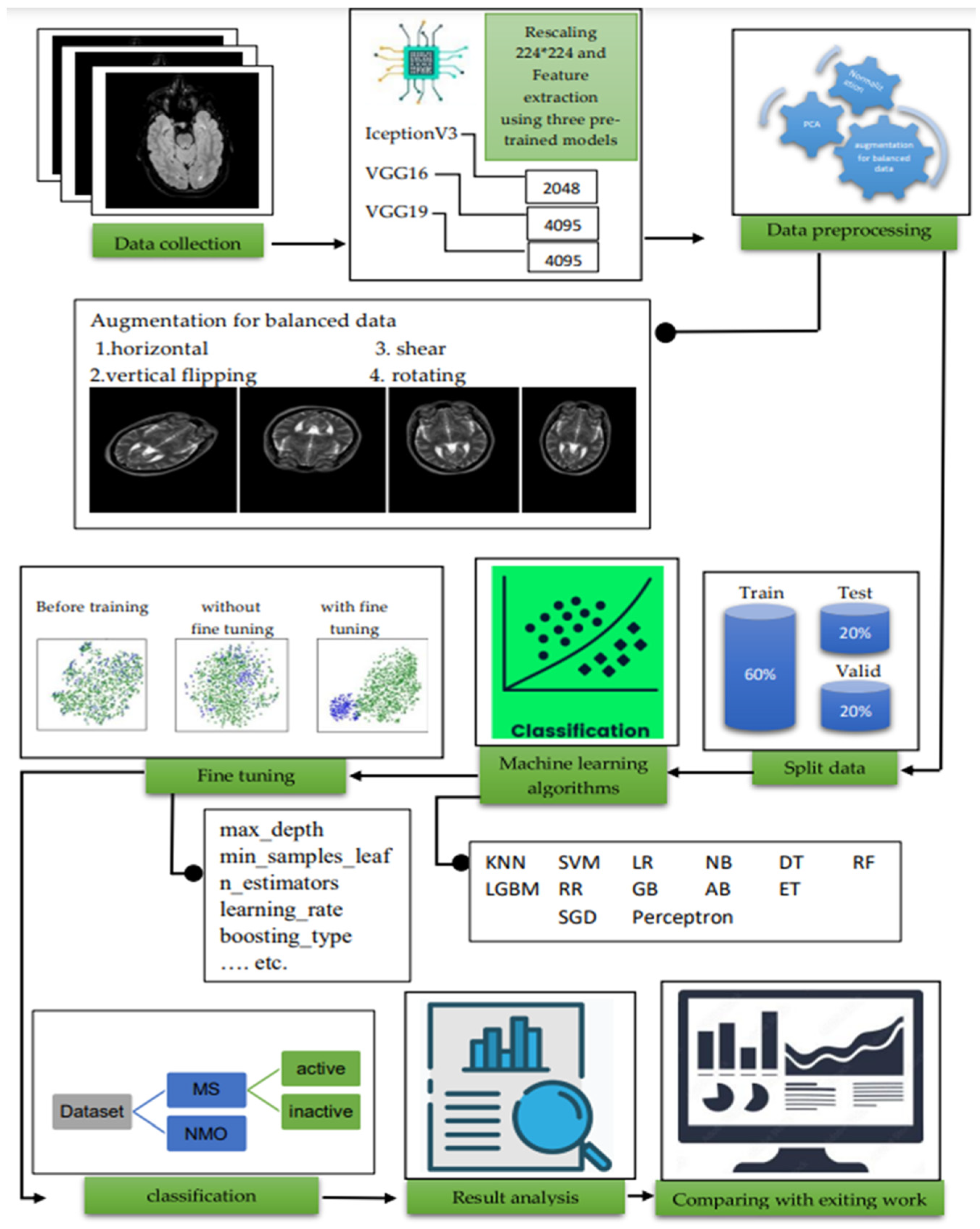
3. Methodology
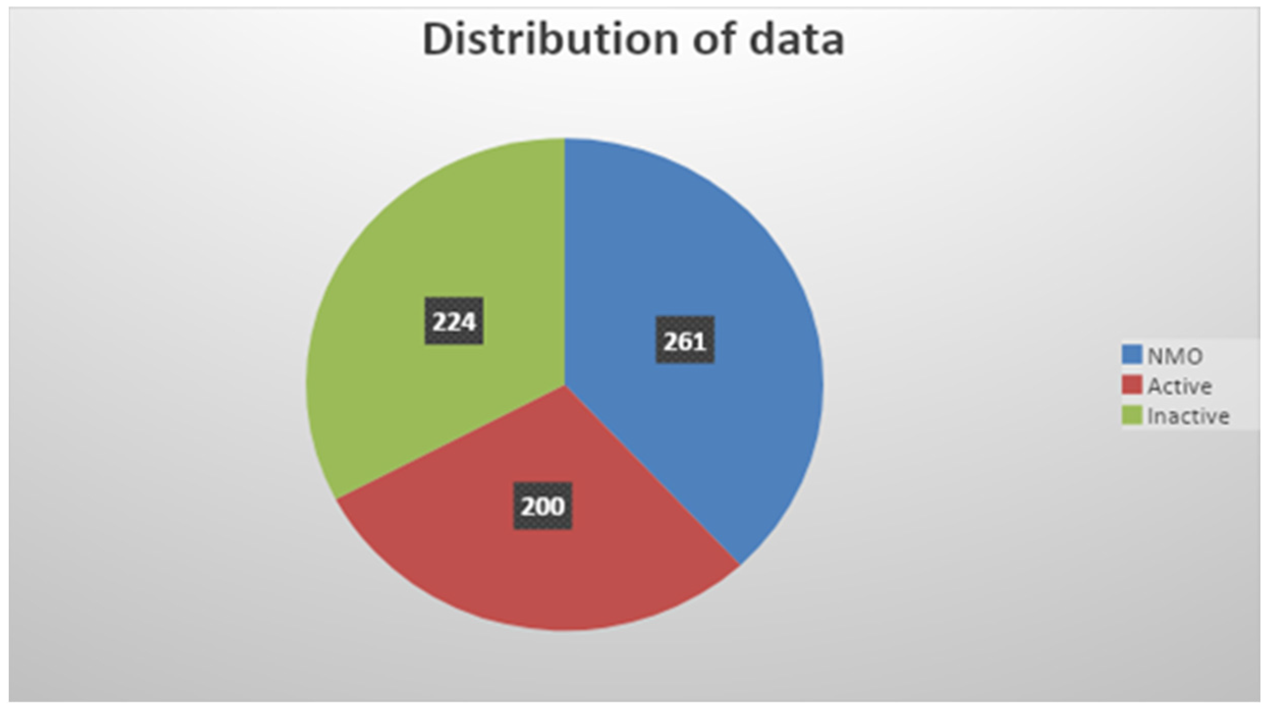
3.1. Data Acquisition
3.1.1. Participants
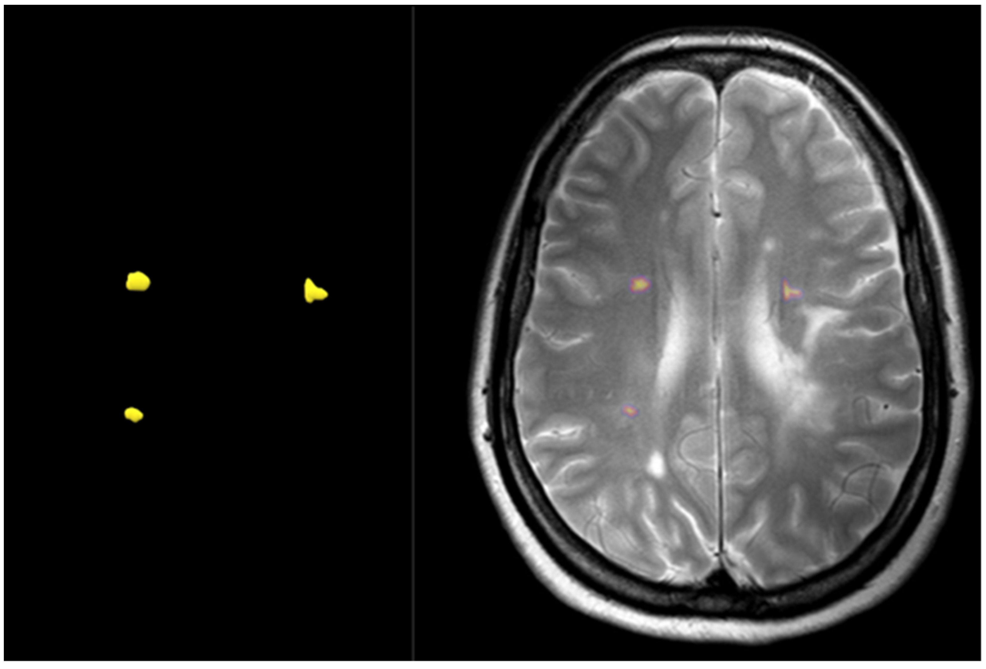
3.1.2. MRI Acquisition
3.1.3. MS vs. NMO Diagnosis
3.2. Pre-Processing
3.2.1. Augmentation
3.2.2. Feature Extraction with Deep Learning Models
3.2.3. Principal Component Analysis
3.2.4. Normalization
3.3. Machine Learning Algorithms
4. Result and Discussion
4.1. Performance Measures and Experiments
- Accuracy: Refers to the correctly expected cases from the sum of all cases as shown in Formula (1):Accuracy = (TP + TN)/(TP + FP + FN + TN) SEQ Equation\* ARABIC
- Precision: Refers to the positive cases that were correctly predicted for all positive cases as shown in Formula (2):Precision = TP/(TP + FP) SEQ Equation\* ARABIC
- Recall: The proportion of predicted true positive cases that were correctly predicted relative to all actual positive cases stated in Formula (3):Recall = TP/(TP + FN) SEQ Equation\* ARABIC
- F1-Score: Balances precision and recall to evaluate overall performance stated in Formula (4):F1-score = 2 × (precision×recall)/(precision + recall) SEQ Equation\* ARABIC
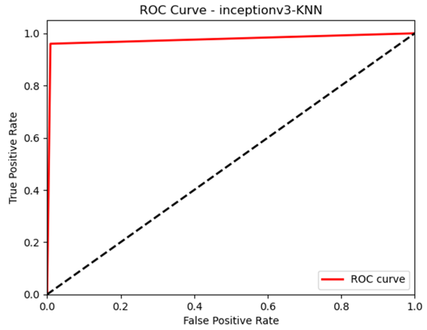
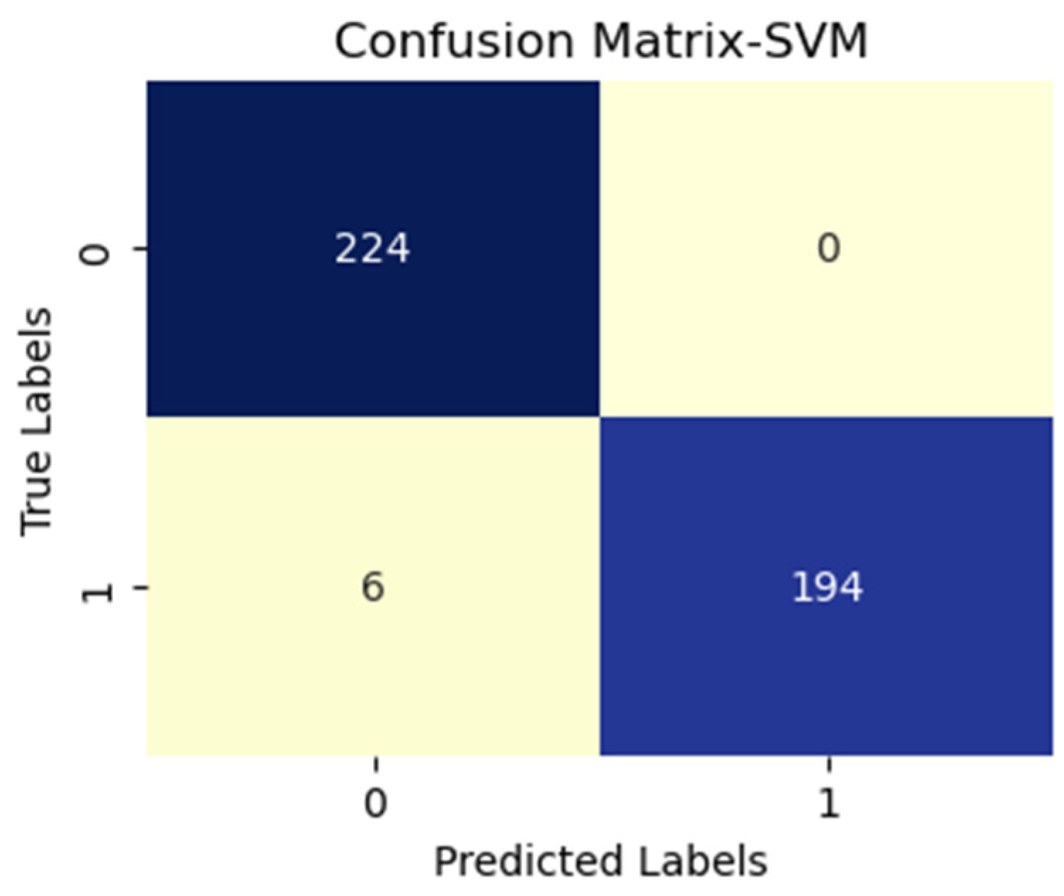
4.2. Result Analysis
4.3. Comparison with Other Studies
5. Conclusions and Recommendations
Author Contributions
Funding
Institutional Review Board Statement
Informed Consent Statement
Data Availability Statement
Conflicts of Interest
Appendix A
- Random Forest (RF)
- Support Vector Machine (SVM)
- Naïve Bayes (NB)
- k-Nearest Neighbor (KNN)
- Logistic Regression
- Decision Tree (DT)
- Extra Trees Classifier
- LightGBM (LGBM)
- Ada Boost
- Gradient Boosting
- Stochastic Gradient Descent (SGD)
- Ridge Regression
References
- Calabresi, P.A. Diagnosis and management of multiple sclerosis. Am. Fam. Physician 2004, 70, 1935–1944. [Google Scholar]
- Goldenberg, M.M. Multiple sclerosis review. Pharm. Ther. 2012, 37, 175. [Google Scholar]
- Brownlee, W.J.; Hardy, T.A.; Fazekas, F.; Miller, D.H. Diagnosis of multiple sclerosis: Progress and challenges. Lancet 2017, 389, 1336–1346. [Google Scholar] [CrossRef]
- Arshad, A.; Jabeen, M.; Ubaid, S.; Raza, A.; Abualigah, L.; Aldiabat, K.; Jia, H. A novel ensemble method for enhancing Internet of Things device security against botnet attacks. Decis. Anal. J. 2023, 8, 100307. [Google Scholar] [CrossRef]
- Ömerhoca, S.; Akkaş, S.Y.; İçen, N.K. Multiple sclerosis: Diagnosis and differential diagnosis. Arch. Neuropsychiatry 2018, 55, S1–S9. [Google Scholar] [CrossRef] [PubMed]
- Lennon, V.A.; Wingerchuk, D.M.; Kryzer, T.J.; Pittock, S.J.; Lucchinetti, C.F.; Fujihara, K.; Weinshenker, B.G. A serum autoantibody marker of neuromyelitis optica: Distinction from multiple sclerosis. Lancet 2004, 364, 2106–2112. [Google Scholar] [CrossRef] [PubMed]
- Kim, W.; Kim, S.H.; Lee, S.H.; Li, X.F.; Kim, H.J. Brain abnormalities as an initial manifestation of neuromyelitis optica spectrum disorder. Mult. Scler. J. 2011, 17, 1107–1112. [Google Scholar] [CrossRef] [PubMed]
- Mandler, R.N.; Ahmed, W.; Dencoff, J.E. Devic’s neuromyelitis optica: A prospective study of seven patients treated with prednisone and azathioprine. Neurology 1998, 51, 1219–1220. [Google Scholar] [CrossRef] [PubMed]
- Kawachi, I.; Lassmann, H. Neurodegeneration in multiple sclerosis and neuromyelitis optica. J. Neurol. Neurosurg. Psychiatry 2017, 88, 137–145. [Google Scholar] [CrossRef]
- Kim, H.; Lee, Y.; Kim, Y.H.; Lim, Y.M.; Lee, J.S.; Woo, J.; Kim, K.K. Deep learning-based method to differentiate neuromyelitis optica spectrum disorder from multiple sclerosis. Front. Neurol. 2020, 11, 599042. [Google Scholar] [CrossRef]
- Miller, D.H.; Albert, P.S.; Barkhof, F.; Francis, G.; Frank, J.A.; Hodgkinson, S.; Lublin, F.D.; Paty, D.W.; Reingold, S.C.; Simon, J. Guidelines for the use of magnetic resonance techniques in monitoring the treatment of multiple sclerosis. Ann. Neurol. 1996, 39, 6–16. [Google Scholar] [CrossRef] [PubMed]
- Goodin, D.S.; Frohman, E.M.; Garmany, G.P.; Halper, J.; Likosky, W.H.; Lublin, F.D. Disease modifying therapies in multiple sclerosis. Neurology 2002, 58, 169–178. [Google Scholar] [PubMed]
- Lassmann, H. Multiple sclerosis pathology. Cold Spring Harb. Perspect. Med. 2018, 8, a028936. [Google Scholar] [CrossRef] [PubMed]
- Moraal, B.; Wattjes, M.P.; Geurts, J.J.G.; Dirk, L.K.; van Schijndel, R.A.; Pouwels, P.J.W.; Vrenken, H.; Barkhof, F. Improved detection of active multiple sclerosis lesions: 3D subtraction imaging. Radiology 2010, 255, 154–163. [Google Scholar] [CrossRef]
- Lladó, X.; Ganiler, O.; Oliver, A.; Martí, R.; Freixenet, J.; Valls, L.; Vilanova, J.C.; Ramió-Torrentà, L.; Rovira, À. Automated detection of multiple sclerosis lesions in serial brain MRI. Neuroradiology 2012, 54, 787–807. [Google Scholar] [CrossRef]
- Buyukturkoglu, K.; Zeng, D.; Bharadwaj, S.; Tozlu, C.; Mormina, E.; Igwe, K.C.; Lee, S.; Habeck, C.; Brickman, A.M.; Riley, C.S.; et al. Classifying multiple sclerosis patients on the basis of SDMT performance using machine learning. Mult. Scler. J. 2021, 27, 107–116. [Google Scholar] [CrossRef]
- Ramanujam, R.; Zhu, F.; Fink, K.; Karrenbauer, V.D.; Lorscheider, J.; Benkert, P.; Kingwell, E.; Tremlett, H.; Hillert, J.; Manouchehrinia, A. Accurate classification of secondary progression in multiple sclerosis using a decision tree. Mult. Scler. J. 2021, 27, 1240–1249. [Google Scholar] [CrossRef]
- Loizou, C.P.; Pantzaris, M.; Pattichis, C.S. Normal appearing brain white matter changes in relapsing multiple sclerosis: Texture image and classification analysis in serial MRI scans. Magn. Reson. Imaging 2020, 73, 192–202. [Google Scholar] [CrossRef]
- Saccà, V.; Sarica, A.; Novellino, F.; Barone, S.; Tallarico, T.; Filippelli, E.; Granata, A.; Chiriaco, C.; Bruno Bossio, R.; Valentino, P.; et al. Evaluation of machine learning algorithms performance for the prediction of early multiple sclerosis from resting-state FMRI connectivity data. Brain Imaging Behav. 2019, 13, 1103–1114. [Google Scholar] [CrossRef]
- Samah, Y.; Yassine, B.S.; Naceur, A.M. Multiple sclerosis lesions detection from noisy magnetic resonance brain images tissue. In Proceedings of the 2018 15th International Multi-Conference on Systems, Signals & Devices (SSD), Yasmine Hammamet, Tunisia, 19–22 March 2018. [Google Scholar]
- Maggi, P.; Fartaria, M.J.; Jorge, J.; La Rosa, F.; Absinta, M.; Sati, P.; Meuli, R.; Du Pasquier, R.; Reich, D.S.; Cuadra, M.B. CVSnet: A machine learning approach for automated central vein sign assessment in multiple sclerosis. NMR Biomed. 2020, 33, e4283. [Google Scholar] [CrossRef]
- Roy, S.; Butman, J.A.; Reich, D.S.; Calabresi, P.A.; Pham, D.L. Multiple sclerosis lesion segmentation from brain MRI via fully convolutional neural networks. arXiv 2018, arXiv:1803.09172. [Google Scholar]
- Sepahvand, N.M.; Arnold, D.L.; Arbel, T. CNN detection of new and enlarging multiple sclerosis lesions from longitudinal MRI using subtraction images. In Proceedings of the 2020 IEEE 17th International Symposium on Biomedical Imaging (ISBI), Iowa City, IA, USA, 3–7 April 2020. [Google Scholar]
- Eshaghi, A.; Wottschel, V.; Cortese, R.; Calabrese, M.; Sahraian, M.A.; Thompson, A.J.; Alexander, D.C.; Ciccarelli, O. Gray matter MRI differentiates neuromyelitis optica from multiple sclerosis using random forest. Neurology 2016, 87, 2463–2470. [Google Scholar] [CrossRef] [PubMed]
- Zhang, H.; Nguyen, T.D.; Zhang, J.; Marcille, M.; Spincemaille, P.; Wang, Y.; Gauthier, S.A.; Sweeney, E.M. QSMRim-Net: Imbalance-aware learning for identification of chronic active multiple sclerosis lesions on quantitative susceptibility maps. NeuroImage Clin. 2022, 34, 102979. [Google Scholar] [CrossRef] [PubMed]
- Coronado, I.; Gabr, R.E.; Narayana, P.A. Narayana. Deep learning segmentation of gadolinium-enhancing lesions in multiple sclerosis. Mult. Scler. J. 2018, 27, 519–527. [Google Scholar] [CrossRef] [PubMed]
- Gaj, S.; Ontaneda, D.; Nakamura, K. Automatic segmentation of gadolinium-enhancing lesions in multiple sclerosis using deep learning from clinical MRI. PLoS ONE 2021, 16, e0255939. [Google Scholar] [CrossRef]
- Narayana, P.A.; Coronado, I.; Sujit, S.J.; Wolinsky, J.S.; Lublin, F.D.; Gabr, R.E. Deep learning for predicting enhancing lesions in multiple sclerosis from noncontrast MRI. Radiology 2020, 294, 398–404. [Google Scholar] [CrossRef]
- Seok, J.M.; Cho, W.; Chung, Y.H.; Ju, H.; Kim, S.T.; Seong, J.K.; Min, J.H. Differentiation between multiple sclerosis and neuromyelitis optica spectrum disorder using a deep learning model. Sci. Rep. 2023, 13, 11625. [Google Scholar] [CrossRef]
- Kavaklioglu, B.C.; Erdman, L.; Goldenberg, A.; Kavaklioglu, C.; Alexander, C.; Oppermann, H.M.; Patel, A.; Hossain, S.; Berenbaum, T.; Yau, O. Machine learning classification of multiple sclerosis in children using optical coherence tomography. Mult. Scler. J. 2022, 28, 2253–2262. [Google Scholar] [CrossRef]
- Kenney, R.C.; Liu, M.; Hasanaj, L.; Joseph, B.; Abu Al-Hassan, A.; Balk, L.J.; Behbehani, R.; Brandt, A.; Calabresi, P.A.; Frohman, E. The role of optical coherence tomography criteria and machine learning in multiple sclerosis and optic neuritis diagnosis. Neurology 2022, 99, e1100–e1112. [Google Scholar] [CrossRef]
- Garcia-Martin, E.; Dongil-Moreno, F.; Ortiz, M.; Ciubotaru, O.; Boquete, L.; Sánchez-Morla, E.; Jimeno-Huete, D.; Miguel, J.; Barea, R.; Vilades, E. Diagnosis of Multiple Sclerosis using Optical Coherence Tomography Supported by Explainable Artificial Intelligence. 2023; Preprint. [Google Scholar] [CrossRef]
- Gharaibeh, M.; Alzu’bi, D.; Abdullah, M.; Hmeidi, I.; Al Nasar, M.R.; Abualigah, L.; Gandomi, A.H. Radiology imaging scans for early diagnosis of kidney tumors: A review of data analytics-based machine learning and deep learning approaches. Big Data Cogn. Comput. 2022, 6, 29. [Google Scholar] [CrossRef]
- Thompson, A.J.; Banwell, B.L.; Barkhof, F.; Carroll, W.M.; Coetzee, T.; Comi, G.; Correale, J.; Fazekas, F.; Filippi, M.; Freedman, M.S.; et al. Diagnosis of multiple sclerosis: 2017 revisions of the McDonald criteria. Lancet Neurol. 2018, 17, 162–173. [Google Scholar] [CrossRef]
- Wingerchuk, D.M.; Banwell, B.; Bennett, J.L.; Cabre, P.; Carroll, W.; Chitnis, T.; De Seze, J.; Fujihara, K.; Greenberg, B.; Jacob, A.; et al. International consensus diagnostic criteria for neuromyelitis optica spectrum disorders. Neurology 2015, 85, 177–189. [Google Scholar] [CrossRef]
- Singer, G.; Marudi, M. Ordinal decision-tree-based ensemble approaches: The case of controlling the daily local growth rate of the COVID-19 epidemic. Entropy 2020, 22, 871. [Google Scholar] [CrossRef] [PubMed]
- Jaradat, A.S.; Al Mamlook, R.E.; Almakayeel, N.; Alharbe, N.; Almuflih, A.S.; Nasayreh, A.; Gharaibeh, H.; Gharaibeh, M.; Gharaibeh, A.; Bzizi, H. Automated Monkeypox Skin Lesion Detection Using Deep Learning and Transfer Learning Techniques. Int. J. Environ. Res. Public Health 2023, 20, 4422. [Google Scholar] [CrossRef] [PubMed]
- Simonyan, K.; Zisserman, A. Very deep convolutional networks for large-scale image recognition. arXiv 2014, arXiv:1409.1556. [Google Scholar]
- Szegedy, C.; Vanhoucke, V.; Ioffe, S.; Shlens, J.; Wojna, Z. Rethinking the inception architecture for computer vision. In Proceedings of the IEEE Conference on Computer Vision and Pattern Recognition (CVPR), Las Vegas, NV, USA, 27–30 June 2016. [Google Scholar]
- Abualigah, L.M.Q. Feature Selection and Enhanced Krill Herd Algorithm for Text Document Clustering; Springer: Cham, Switzerland, 2019; p. 816. [Google Scholar]
- Fonville, J.M.; Carter, C.; Cloarec, O.; Nicholson, J.K.; Lindon, J.C.; Bunch, J.; Holmes, E. Robust data processing and normalization strategy for MALDI mass spectrometric imaging. Anal. Chem. 2012, 84, 1310–1319. [Google Scholar] [CrossRef]
- Otair, M.; Ibrahim, O.T.; Abualigah, L.; Altalhi, M.; Sumari, P. An enhanced grey wolf optimizer based particle swarm optimizer for intrusion detection system in wireless sensor networks. Wirel. Netw. 2022, 28, 721–744. [Google Scholar] [CrossRef]
- Khaledian, N.; Nazari, A.; Khamforoosh, K.; Abualigah, L.; Javaheri, D. TrustDL: Use of trust-based dictionary learning to facilitate recommendation in social networks. Expert Syst. Appl. 2023, 228, 120487. [Google Scholar] [CrossRef]
- Musleh, D.; Alotaibi, M.; Alhaidari, F.; Rahman, A.; Mohammad, R.M. Intrusion Detection System Using Feature Extraction with Machine Learning Algorithms in IoT. J. Sens. Actuator Netw. 2023, 12, 29. [Google Scholar] [CrossRef]
- Selvanayaki, K.S.; Somasundaram, R.; Shyamala, D.J. Detection and Recognition of Vehicle Using Principal Component Analysis. In Proceedings of the International Conference on ISMAC in Computational Vision and Bio-Engineering 2018 (ISMAC-CVB); Springer: Cham, Switzerland, 2019; p. 30. [Google Scholar]
- Al-Manaseer, H.; Abualigah, L.; Alsoud, A.R.; Zitar, R.A.; Ezugwu, A.E.; Jia, H. A novel big data classification technique for healthcare application using support vector machine, random forest and J48. In Classification Applications with Deep Learning and Machine Learning Technologies; Springer: Cham, Switzerland, 2023; Volume 1071, pp. 205–215. [Google Scholar]
- Houssein, E.H.; Dirar, M.; Abualigah, L.; Mohamed, W.M. An efficient equilibrium optimizer with support vector regression for stock market prediction. Neural Comput. Appl. 2022, 34, 3165–3200. [Google Scholar] [CrossRef]
- Leung, K.M. Naive Bayesian Classifier, Department of Computer Science/Finance and Risk Engineering, Polytechnic University. 2007. Available online: https://cse.engineering.nyu.edu/~mleung/FRE7851/f07/naiveBayesianClassifier.pdf (accessed on 2 July 2023).
- Abualigah, L. Classification Applications with Deep Learning and Machine Learning Technologies; Springer: Cham, Switzerland, 2022; p. 1071. [Google Scholar]
- Friedman, J.H. Stochastic gradient boosting. Comput. Stat. Data Anal. 2002, 38, 367–378. [Google Scholar] [CrossRef]
- LeCun, Y.; Bottou, L.; Orr, G.B.; Müller, K.R. Efficient backprop. In Neural Networks: Tricks of the Trade; Springer: Berlin/Heidelberg, Germany, 2002; pp. 9–50. [Google Scholar]
- Hastie, T.; Tibshirani, R.; Friedman, J.H.; Friedman, J.H. The Elements of Statistical Learning: Data Mining, Inference, and Prediction; Springer: Berlin/Heidelberg, Germany, 2009; Volume 2. [Google Scholar]


| Author | Data | Approaches | Results |
|---|---|---|---|
| [16] | 183 MRI | Random forest | AUC: 90% |
| [17] | 14387 MS | Decision tree | Accuracy: 89.5% |
| [18] | MRI images MS | SVM | Accuracy of (NAWM0 vs. ROISC0): 89% (NAWM0 vs. NAWM6-12): 95% (NAWM0 vs L0): 98% (NAWM6-12 vs. L6-12): 92% (ROIS0 vs. L0): 95% (ROIS0 vs. L6-12): 90% (ROIS0 vs. ROISC0): 65% |
| [19] | clinical data based on MR images | ANN, SVM, KNN, naïve Bayes, random forest | Accuracy of SVM and random forest: 85.7% |
| [20] | MRI images MS | SVM with DDP for analyzes the MRI images | Accuracy: T1: 97.12% T2: 94.21% |
| [21] | 80 dataset MRI | 3DCNN (CVSnet) | Accuracy: 91% |
| [22] | 100 dataset MS ISBI 2015 challenge (14 patients) | CNN (segmentation) | Score: 90.48 |
| [23] | 35 patients with MS and 18 patients with NMOSD | CNN with SqueezeNet | Accuracy: 81.1% Sensitivity of MS: 80.0%, Sensitivity of NMOSD: 83.3% |
| [24] | 90 patients with MS and NMO | Random forest | Accuracy: MS vs. HCs: 92% NMO vs. HCs: 88% |
| [25] | 172 MRI MS for detecting Active | QSMRim-Net | AUC: 0.760 |
| [26] | 1006 patients MRI to detect Active | CNN (U5) | DSC: 0.77 TPR: 0.90 FPR: 0.23 |
| [27] | 600 MRI for Active | 2D Unet, random forest | Accuracy: 87.7% |
| [28] | 1008 patients MRI for Active | VGG16 | AUCs: Slice-wise: 0.82 ± 0.02 Participant-wise enhancement: 0.75 ± 0.03 |
| [29] | 1677 different scans of MRI active and inactive | 3D Unet | AUC: 0.95 Sensitivities: 0.69 Specificities: 0.97 |
| [33] | MRI images | ResNet18 and Grad-CAM | Accuracy: 76.1%, sensitivity: 77.3%, specificity: 74.8%, |
| [30] | 512 eyes from 187 patients | Random forest | Accuracy: 80% for MS 75% for demyelinating diseases |
| [31] | 1568 PwMS and 552 controls | SVM | (AUC) = 0.89 (95% CI 0.85–0.93) sensitivity = 81%, and specificity = 80% |
| [32] | 79 patients | SVM-RFE-LOOCV | Sensitivity = 0.86 specificity = 0.90 |
| MS | NMO | p-Value | |
|---|---|---|---|
| Gender ratio (F/M) | 2/1 | 5/1 | 0.758 |
| Age (years), mean ± SD | 45 ± 14.90 | 30 ± 30.66 | 0.743 |
| Disease duration (years), mean ± SD | 9.20 ± 7.14 | 6.16 ± 9.26 | 0.705 |
| CNN Models for Feature Extraction | Machine Learning Algorithms | Precision | Recall | F1-Score | Accuracy |
|---|---|---|---|---|---|
| VGG16 | Logistic regression | 0.78 | 0.71 | 0.74 | 0.75 |
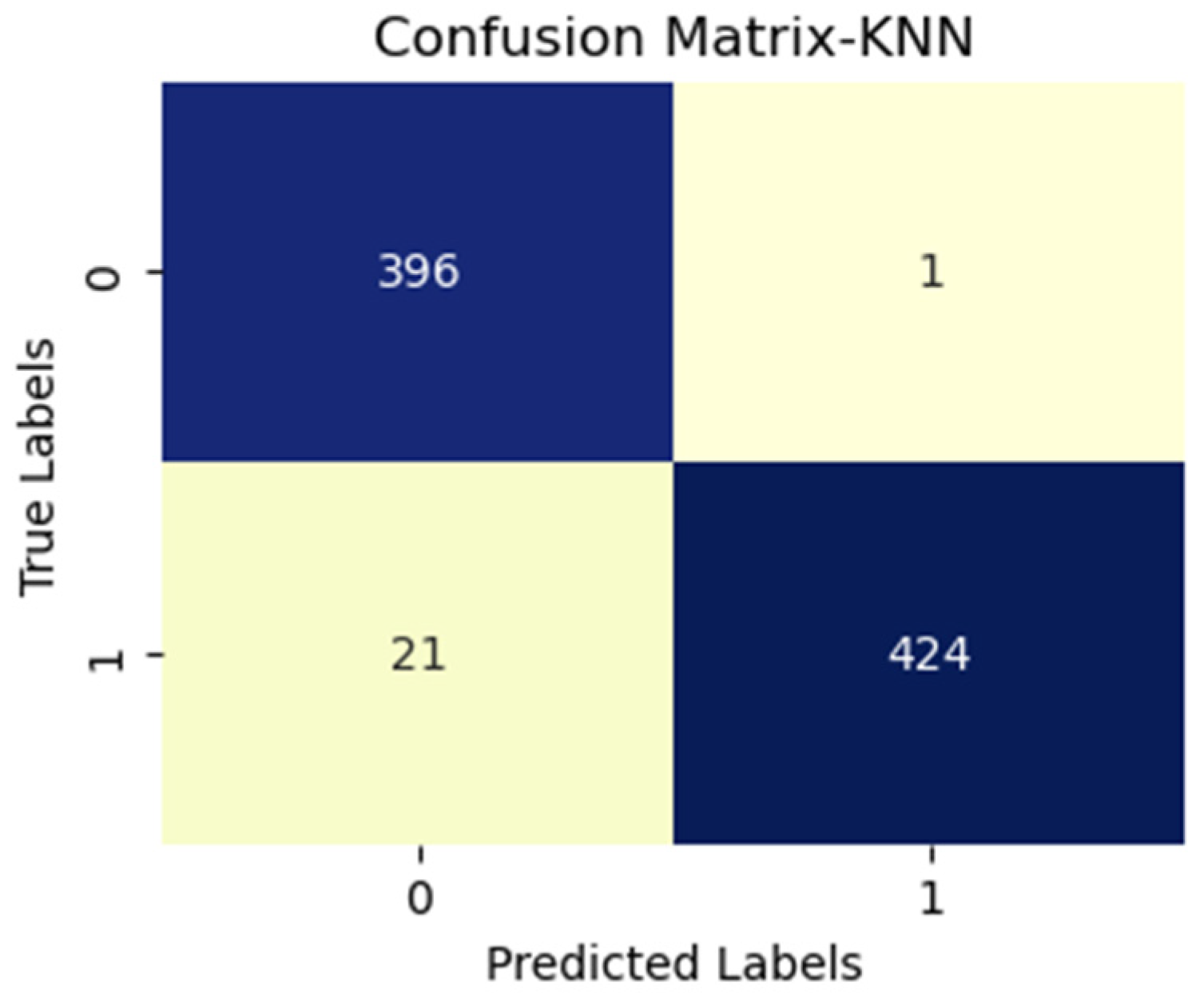
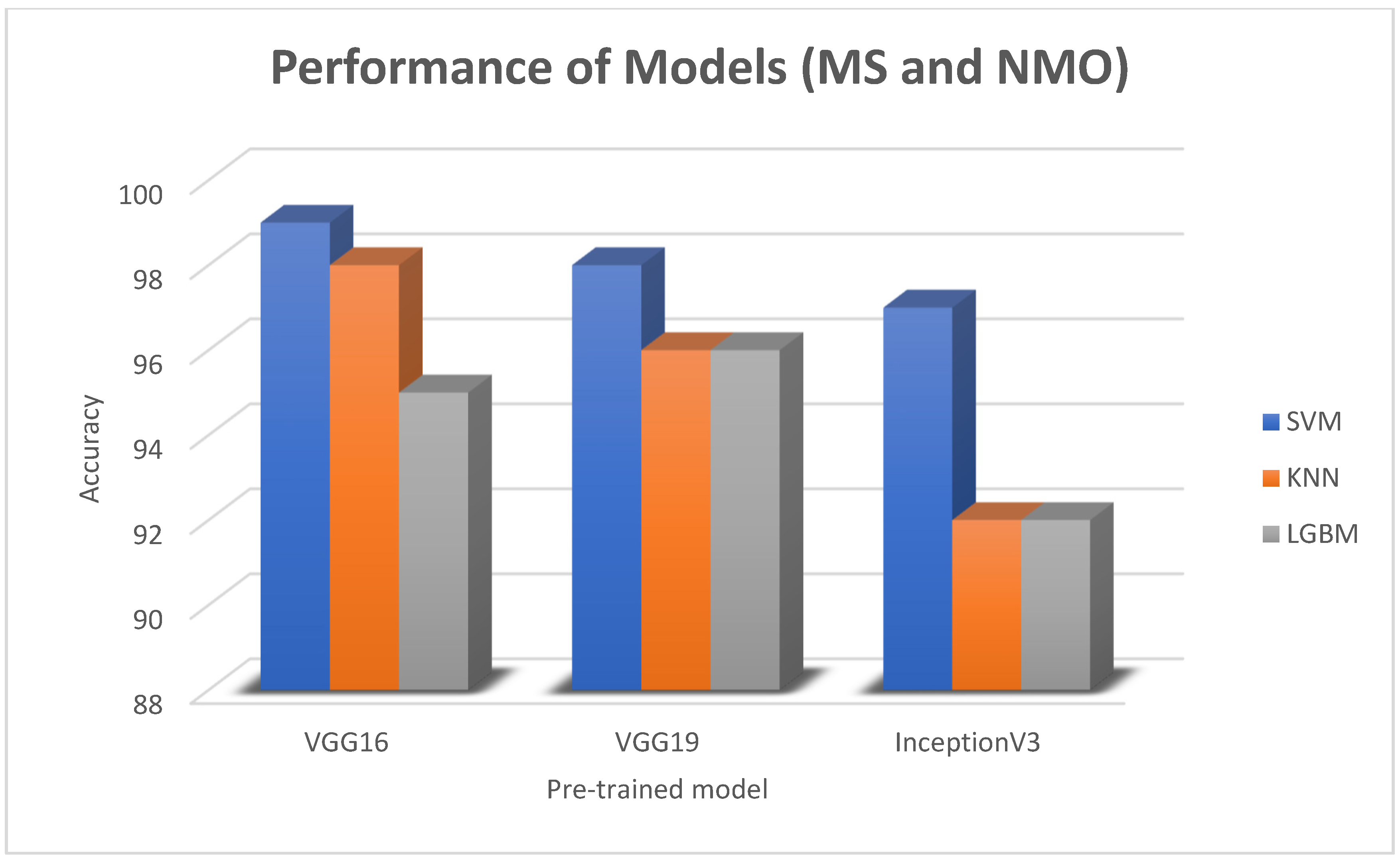
| KNN | 0.98 | 0.99 | 0.99 | 0.99 | |
| SVM | 0.99 | 0.97 | 0.96 | 0.96 | |
| Naïve Bayes | 0.71 | 0.61 | 0.66 | 0.68 | |
| DT | 0.78 | 0.74 | 0.76 | 0.76 | |
| Perceptron | 0.76 | 0.59 | 0.66 | 0.70 | |
| Stochastic gradient descent | 0.84 | 0.59 | 0.70 | 0.74 | |
| RF | 0.94 | 0.89 | 0.92 | 0.92 | |
| Extra trees classifier | 0.95 | 0.71 | 0.81 | 0.80 | |
| Gradient boost | 0.96 | 0.93 | 0.94 | 0.94 | |
| Ada boost | 0.80 | 0.68 | 0.74 | 0.75 | |
| Ridge regression | 0.77 | 0.68 | 0.72 | 0.73 | |
| LGBM | 0.95 | 0.90 | 0.93 | 0.93 | |
| VGG19 | Logistic regression | 0.80 | 0.74 | 0.77 | 0.77 |
| KNN | 0.96 | 0.98 | 0.97 | 0.97 | |
| SVM | 0.98 | 0.93 | 0.95 | 0.95 | |
| Naïve Bayes | 0.74 | 0.68 | 0.71 | 0.72 | |
| DT | 0.72 | 0.72 | 0.72 | 0.72 | |
| Perceptron | 0.76 | 0.64 | 0.70 | 0.72 | |
| Stochastic gradient descent | 0.76 | 0.76 | 0.76 | 0.76 | |
| RF | 0.96 | 0.90 | 0.93 | 0.93 | |
| Extra trees classifier | 0.97 | 0.75 | 0.85 | 0.86 | |
| Gradient boost | 0.96 | 0.90 | 0.93 | 0.93 | |
| Ada boost | 0.80 | 0.71 | 0.75 | 0.76 | |
| Ridge regression | 0.81 | 0.72 | 0.76 | 0.77 | |
| LGBM | 0.96 | 0.91 | 0.94 | 0.94 | |
| InceptionV3 | Logistic regression | 0.80 | 0.76 | 0.78 | 0.78 |
| KNN | 0.92 | 0.95 | 0.93 | 0.93 | |
| SVM | 0.97 | 0.89 | 0.92 | 0.93 | |
| Naïve Bayes | 0.74 | 0.64 | 0.69 | 0.71 | |
| Perceptron | 0.68 | 0.73 | 0.71 | 0.69 | |
| Stochastic gradient descent | 0.77 | 0.78 | 0.78 | 0.77 | |
| DT | 0.72 | 0.72 | 0.72 | 0.71 | |
| Extra trees classifier | 0.93 | 0.79 | 0.85 | 0.86 | |
| Gradient boost | 0.92 | 0.86 | 0.89 | 0.89 | |
| Ridge regression | 0.91 | 0.72 | 0.77 | 0.78 | |
| Ada boost | 0.76 | 0.74 | 0.75 | 0.75 | |
| LGBM | 0.92 | 0.88 | 0.90 | 0.90 |
| CNN Models for Feature Extraction | Machine Learning Algorithms | Precision | Recall | F1-Score | Accuracy |
|---|---|---|---|---|---|
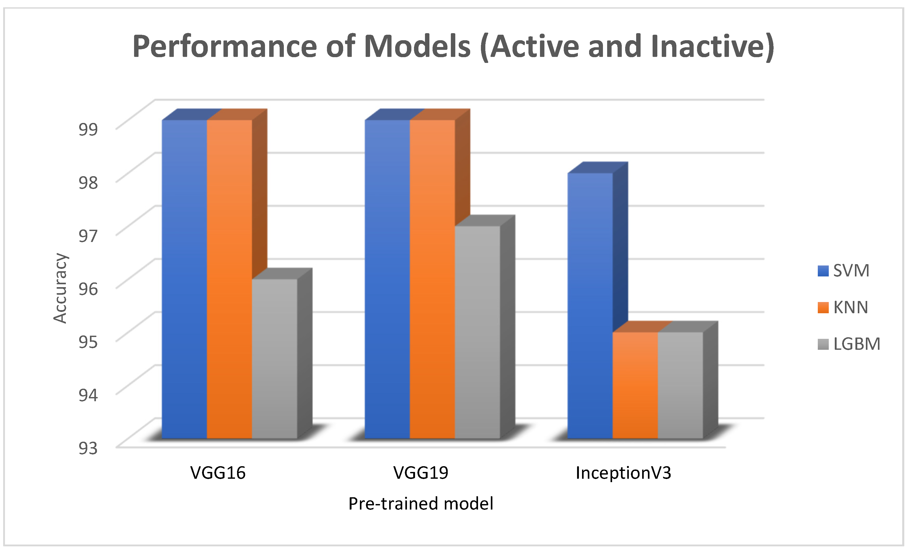
| VGG16 | Logistic regression | 0.90 | 0.86 | 0.88 | 0.89 |
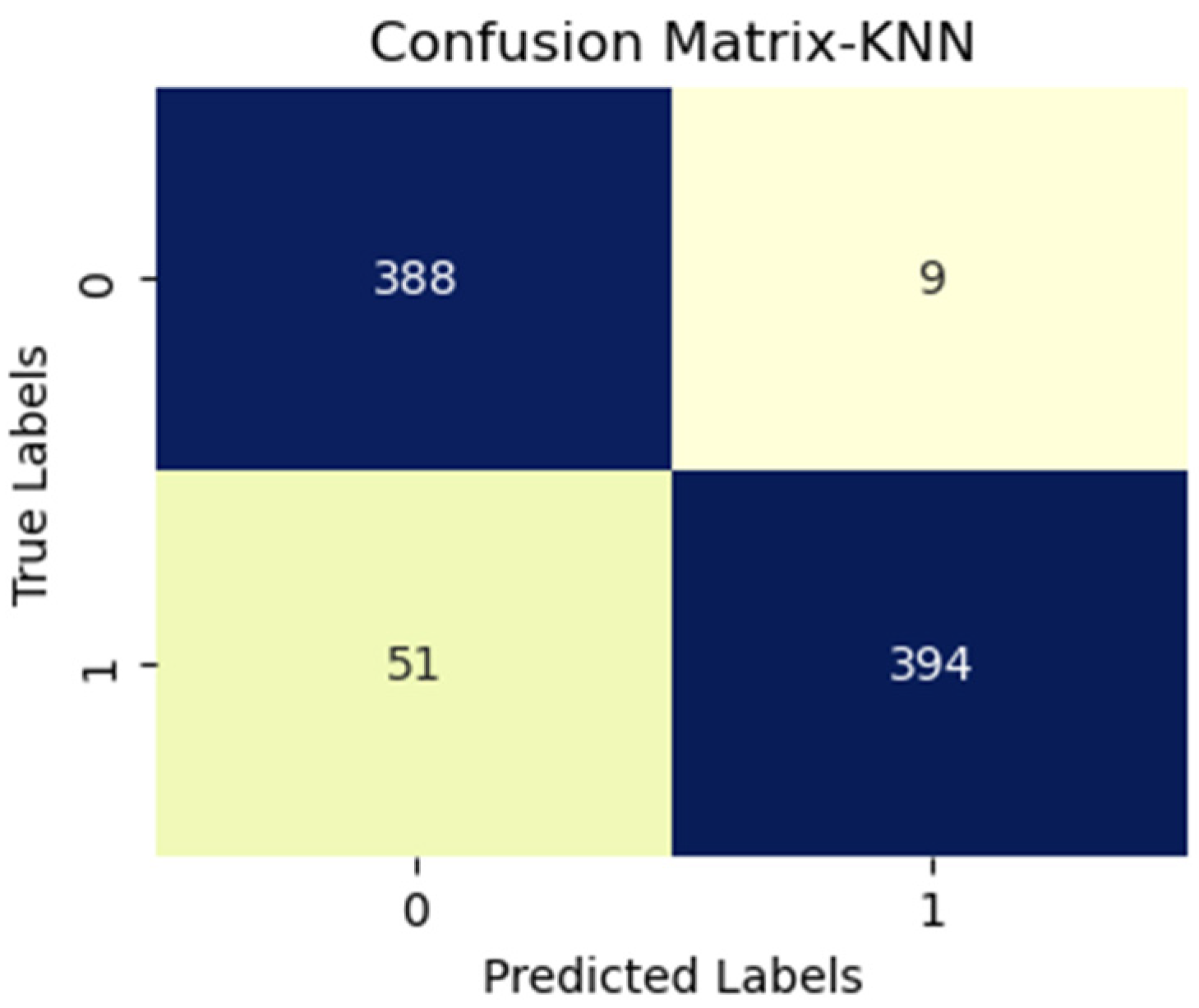
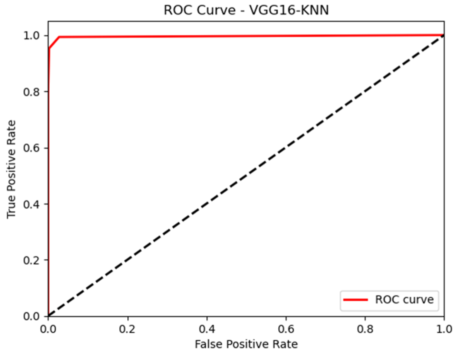
| KNN | 0.99 | 0.96 | 0.98 | 0.98 | |
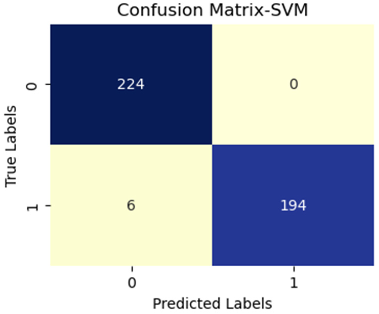
| SVM | 0.99 | 0.97 | 0.98 | 0.98 | |
| Naïve Bayes | 0.85 | 0.79 | 0.82 | 0.83 | |
| DT | 0.80 | 0.75 | 0.77 | 0.79 | |
| Perceptron | 0.91 | 0.80 | 0.85 | 0.86 | |
| Stochastic gradient descent | 0.78 | 0.91 | 0.89 | 0.89 | |
| RF | 0.96 | 0.94 | 0.95 | 0.95 | |
| Extra trees classifier | 0.95 | 0.95 | 0.95 | 0.95 | |
| Gradient boost | 0.96 | 0.96 | 0.96 | 0.96 | |
| Ada boost | 0.80 | 0.82 | 0.81 | 0.81 | |
| Ridge regression | 0.89 | 0.86 | 0.88 | 0.88 | |
| LGBM | 0.96 | 0.97 | 0.97 | 0.97 | |
| VGG19 | Logistic regression | 0.90 | 0.86 | 0.88 | 0.89 |
| KNN | 0.99 | 0.96 | 0.97 | 0.97 | |
| SVM | 0.99 | 0.98 | 0.98 | 0.98 | |
| Naïve Bayes | 0.86 | 0.79 | 0.82 | 0.83 | |
| DT | 0.80 | 0.79 | 0.79 | 0.80 | |
| Perceptron | 0.88 | 0.86 | 0.87 | 0.87 | |
| Stochastic gradient descent | 0.87 | 0.88 | 0.87 | 0.88 | |
| RF | 0.96 | 0.95 | 0.95 | 0.96 | |
| Extra trees classifier | 0.96 | 0.97 | 0.96 | 0.96 | |
| Gradient boost | 0.95 | 0.95 | 0.95 | 0.95 | |
| Ada boost | 0.78 | 0.81 | 0.79 | 0.79 | |
| Ridge regression | 0.90 | 0.86 | 0.88 | 0.88 | |
| LGBM | 0.97 | 0.95 | 0.96 | 0.96 | |
| InceptionV3 | Logistic regression | 0.89 | 0.86 | 0.87 | 0.88 |
| KNN | 0.98 | 1.00 | 0.98 | 0.98 | |
| SVM | 0.98 | 0.97 | 0.97 | 0.97 | |
| Naïve Bayes | 0.88 | 0.78 | 0.82 | 0.84 | |
| Perceptron | 0.83 | 0.85 | 0.84 | 0.84 | |
| Stochastic gradient descent | 0.89 | 0.86 | 0.88 | 0.88 | |
| DT | 0.76 | 0.71 | 0.73 | 0.75 | |
| Extra trees classifier | 0.94 | 0.92 | 0.93 | 0.93 | |
| RF | 0.96 | 0.91 | 0.94 | 0.94 | |
| Gradient boost | 0.94 | 0.86 | 0.90 | 0.91 | |
| Ridge regression | 0.89 | 0.87 | 0.88 | 0.88 | |
| Ada boost | 0.84 | 0.82 | 0.83 | 0.83 | |
| LGBM | 0.95 | 0.88 | 0.91 | 0.92 |
| Ref | Data | Methodology | Results |
|---|---|---|---|
| [24] | 90 patients with MS and NMO | Random forest | Accuracy: MS vs. HCs: 92% NMO vs. HCs: 88% |
| [18] | MRI images MS | SVM | Accuracy: (NAWM0 vs. L0): 98% |
| [20] | MRI images MS | SVM with DDP for analyzes the MRI images | Accuracy: T1: 97.12% T2: 94.21% |
| The proposed method | MS and NMO images | VGG16 + KNN | Accuracy: 99% |
| Ref | Data | Methodology | Results |
|---|---|---|---|
| [38] | 1677 different scans of MRI active and inactive | 3D Unet | AUC: 0.95 |
| [28] | 1008 patients MRI for active | VGG16 | AUCs: slice-wise: 0.82 ± 0.02 |
| [27] | 600 MRI for active | 2D Unet, random forest | Accuracy: 87.7% |
| The proposed method | Active and inactive images | VGG16 + SVM | Accuracy: 98% |
Disclaimer/Publisher’s Note: The statements, opinions and data contained in all publications are solely those of the individual author(s) and contributor(s) and not of MDPI and/or the editor(s). MDPI and/or the editor(s) disclaim responsibility for any injury to people or property resulting from any ideas, methods, instructions or products referred to in the content. |
© 2023 by the authors. Licensee MDPI, Basel, Switzerland. This article is an open access article distributed under the terms and conditions of the Creative Commons Attribution (CC BY) license (https://creativecommons.org/licenses/by/4.0/).
Share and Cite
Gharaibeh, M.; Abedalaziz, W.; Alawad, N.A.; Gharaibeh, H.; Nasayreh, A.; El-Heis, M.; Altalhi, M.; Forestiero, A.; Abualigah, L. Optimal Integration of Machine Learning for Distinct Classification and Activity State Determination in Multiple Sclerosis and Neuromyelitis Optica. Technologies 2023, 11, 131. https://doi.org/10.3390/technologies11050131
Gharaibeh M, Abedalaziz W, Alawad NA, Gharaibeh H, Nasayreh A, El-Heis M, Altalhi M, Forestiero A, Abualigah L. Optimal Integration of Machine Learning for Distinct Classification and Activity State Determination in Multiple Sclerosis and Neuromyelitis Optica. Technologies. 2023; 11(5):131. https://doi.org/10.3390/technologies11050131
Chicago/Turabian StyleGharaibeh, Maha, Wlla Abedalaziz, Noor Aldeen Alawad, Hasan Gharaibeh, Ahmad Nasayreh, Mwaffaq El-Heis, Maryam Altalhi, Agostino Forestiero, and Laith Abualigah. 2023. "Optimal Integration of Machine Learning for Distinct Classification and Activity State Determination in Multiple Sclerosis and Neuromyelitis Optica" Technologies 11, no. 5: 131. https://doi.org/10.3390/technologies11050131
APA StyleGharaibeh, M., Abedalaziz, W., Alawad, N. A., Gharaibeh, H., Nasayreh, A., El-Heis, M., Altalhi, M., Forestiero, A., & Abualigah, L. (2023). Optimal Integration of Machine Learning for Distinct Classification and Activity State Determination in Multiple Sclerosis and Neuromyelitis Optica. Technologies, 11(5), 131. https://doi.org/10.3390/technologies11050131