The Fractional Step Method versus the Radial Basis Functions for Option Pricing with Correlated Stochastic Processes

Abstract

In option pricing models with correlated stochastic processes, an option premium is commonly a solution to a partial differential equation (PDE) with mixed derivatives in more than two space dimensions. Alternating direction implicit (ADI) finite difference methods are popular for solving a PDE with more than two space dimensions; however, it is not straightforward to employ the ADI method for solving a PDE with mixed derivatives. The aim of this study is to find out which numerical method would be appropriate to solve PDEs with mixed derivatives based on the accuracy of the solutions and the computation time. This study applies the fractional step method and the radial basis functions to solve a PDE with a mixed derivative, and investigates the efficiency of these numerical methods. Numerical experiments are conducted by applying these methods to exchange option pricing; exchange options are selected because the exchange option premium has an analytical form. The numerical results show that the both methods calculate premiums with high accuracy in the presence of mixed derivatives. The fractional step method calculates the option premium more accurately and much faster than the radial basis functions. Therefore, from the numerical experiments, this study concludes that the fractional step method is more appropriate than the radial basis functions for solving a PDE with a mixed derivative.

1. Introduction

Many financial option models are formulated using two or more stochastic processes. Margrabe (1978) derived a valuation formula for exchange option, which is a function of two stochastic asset prices. Heston (1993) developed an equity option pricing model in which the logarithm of an equity price follows a Wiener process with stochastic volatility. Amin and Jarrow (1992) formulated an equity option pricing model with a stochastic equity price and the stochastic risk-free interest rate. Heath et al. (1992) proposed a multi-factor risk-free interest rate model. Lando (1998) evaluated credit derivatives with a stochastic default intensity and the stochastic risk-free interest rate. In these models, option premiums are given as solutions to partial differential equations (PDEs) with mixed derivatives in two or more space dimensions.

PDEs seldom have analytical solutions and hence, numerical procedures are essential to calculate option premiums. Various numerical methods have been applied to option pricing, including tree models (Shreve 2004), finite difference methods (Duffy 2006), and Monte Carlo simulations (Jäckel 2002), among others. When option pricing models are formulated using two or more stochastic processes, correlations between the stochastic processes affect option premiums. However, numerical procedures for correlated stochastic processes are not straightforward. The construction of a correlated tree is not a simple task. Correlated stochastic processes introduce mixed derivatives to PDEs. Among the finite difference methods, the alternating direction implicit (ADI) finite difference method is popular in finance studies; however, the original ADI method is unable to solve PDEs with mixed derivatives (Duffy 2006, p. 224). Monte Carlo simulation can generate correlated random variables; however, it is a time-consuming way to obtain accurate option premiums. Thus, it is essential to establish efficient methods to solve PDEs with mixed derivatives.

The purpose of this study is to examine the accuracy of the solutions and the computation time for solving PDEs with mixed derivatives. In this study, the fractional step method and the radial basis function are used as the basis of the numerical methods. The fractional step method is unfamiliar in the field of finance research, which usually employs the ADI finite difference method to solve PDEs with two or more space dimensions. As noted above, it is not a straightforward process to use the ADI finite difference method to solve PDEs with mixed derivatives.1 The radial basis functions, also known as the meshfree method, were not used until 2000; since then, however, they have become very popular among researchers in many fields (see, e.g., Fasshauer 2007; Liu 2009; Liu and Gu 2005). The radial basis functions are easy to implement, even in higher space dimensions. Thus, the fractional step method and the radial basis functions are applied to solve PEDs with mixed derivatives. Both numerical methods are conducted to evaluate the exchange option premium; the exchange option premium is a solution to a PDE with mixed derivatives, and an analytical solution for the exchange option is known. Therefore, exchange options are suitable as a benchmark to evaluate the efficiency of the numerical methods.

The rest of the paper is organized as follows. Section 2 explains payoffs of exchange options and presents the analytical pricing formula for exchange option. The fractional step method and the radial basis functions are reviewed to solve a PDE with mixed derivatives in Section 3 and Section 4, respectively. The drawback of the ADI method is also explained in Section 3. Section 5 presents the results from numerical experiments, which examine the accuracy and computation time of the fractional step method and the radial basis functions. Both numerical methods are applied to pricing of exchange options. Section 5.1 describes the general setting for the numerical experiments. Section 5.2 investigates the sufficient number of partitions of the space dimensions to obtain the accurate numerical results. The calculation times are examined in this subsection. Section 5.3 investigates the accuracy of both numerical methods for various correlations. Section 6 concludes.

2. Exchange Option

An exchange option allows its holder to exchange one asset for another. Consider an exchange option to exchange stock 2 for stock 1 at maturity, $T$. Payoff at maturity, $f_T$, is expressed as

$$f_T=\max \left(0,S_{1,T}-S_{2,T}\right).$$

(1)

The exchange option premium is calculated using the Black–Scholes model (Margrabe 1978). In the Black–Scholes framework, the time evolution of a stock price follows a log-normal distribution,

$$d\left(\log S_i\right)=\left(r-\frac{1}{2}{\sigma }_i{}^2\right)dt+{\sigma }_{i}d{W}_{i,t},$$

(2)

where $r$ is the risk-free rate, ${\sigma }_i$ is its volatility, and $W_{i,t}$ is a Wiener process under a martingale measure $(i=1,2)$. The correlation between Wiener processes is ${\rho }_{12},$

$$⟨d{W}_{1,t},d{W}_{2,t}⟩={\rho }_{12}dt,$$

(3)

where $⟨,⟩$ stands for a quadratic variation. Stochastic calculus and the arbitrage condition show that the time-$t$ exchange option premium, $f$, satisfies the following PDE,

$$\frac{\partial f}{\partial t}+\frac{1}{2}{\sigma }_1{}^2\frac{{\partial }^{2}f}{\partial x_1{}^2}+{\rho }_{12}{\sigma }_1{\sigma }_2\frac{{\partial }^{2}f}{\partial x_1\partial x_2}+\frac{1}{2}{\sigma }_2{}^2\frac{{\partial }^{2}f}{\partial x_2{}^2}+\left(r-\frac{1}{2}{\sigma }_1{}^2\right)\frac{\partial f}{\partial x_1}+\left(r-\frac{1}{2}{\sigma }_2{}^2\right)\frac{\partial f}{\partial x_2}-rf=0$$

(4)

where $x_i=\log (S_i)$ $(i=1,2)$ is a logarithm transformed price. A pricing formula is developed by Margrabe (1978) as,

$$f=S_{1}N(d^{(+)})-S_{2}N(d^{(-)}), d^{(\pm )}=\frac{\ln \frac{S_1}{S_2}\pm \frac{1}{2}{\sigma }^2\tau }{\sigma \sqrt{\tau }}, {\sigma }^2={\sigma }_1{}^2-2{\rho }_{12}{\sigma }_1{\sigma }_2+{\sigma }_2{}^2$$

(5)

Section 3 and Section 4 explain the fractional step method and the radial basis functions, respectively. In these sections, the PDE in two space dimensions is written as

$$\frac{\partial f}{\partial t}+A_{11}\frac{{\partial }^{2}f}{\partial x_1{}^2}+2A_{12}\frac{{\partial }^{2}f}{\partial x_1\partial x_2}+A_{22}\frac{{\partial }^{2}f}{\partial x_2{}^2}+B_1\frac{\partial f}{\partial x_1}+B_2\frac{\partial f}{\partial x_2}+Cf=0$$

(6)

which includes the PDE, as can be seen in Equation (4). The terminal time condition is given as intrinsic values of the exchange option. The boundary conditions for space variables are set following Jeong and Kim (2013),

$$\frac{{\partial }^{2}f}{\partial x_1{}^2}(x_{1,L},x_2,t)=\frac{{\partial }^{2}f}{\partial x_1{}^2}(x_{1,U},x_2,t)=\frac{{\partial }^{2}f}{\partial x_2{}^2}(x_1,x_{2,L},t)=\frac{{\partial }^{2}f}{\partial x_2{}^2}(x_1,x_{2,U},t)=0$$

(7)

where $x_{i,L}$ and $x_{i,U}$ are the lower and upper bounds of space variables, respectively $(i=1,2)$.

3. The Fractional Step Method

The fractional step method is a variation of the finite difference methods. The fractional step method was developed by Yanenko and his collaborators (Yanenko 1971). As far as we are concerned, few previous studies applied the fractional step method to option pricing: American option pricing (Ikonen and Toivanen 2007) and barrier option pricing (Itkin and Carr 2008; Toivanen 2010).

First, the finite difference method is reviewed to explain the fractional step method. Again, consider a PDE,

$$\frac{\partial u}{\partial t}=A_{xx}\frac{{\partial }^{2}u}{\partial x^2}+2A_{xy}\frac{{\partial }^{2}u}{\partial x\partial y}+A_{yy}\frac{{\partial }^{2}u}{\partial y^2}+B_x\frac{\partial u}{\partial x}+B_y\frac{\partial u}{\partial y}+Cu,$$

(8)

$0\le t\le T$, $x_L\le x\le x_U$, and $y_L\le y\le y_U$, with an initial condition,

$$u(0,x,y)=g(x,y),$$

(9)

and boundary conditions,

$$\underset{x\to x_L}{\lim }\frac{{\partial }^{2}u}{\partial x^2}(t,x,y)=0,\hspace{1em}\underset{x\to x_U}{\lim }\frac{{\partial }^{2}u}{\partial x^2}(t,x,y)=0,$$

(10)

$$\underset{y\to y_L}{\lim }\frac{{\partial }^{2}u}{\partial y^2}(t,x,y)=0,\hspace{1em}\underset{y\to y_U}{\lim }\frac{{\partial }^{2}u}{\partial y^2}(t,x,y)=0$$

(11)

To find a solution to Equation (8) using a numerical procedure, the time axis is discretized as

$$t_n=n\left(\Delta t\right),\hspace{1em}n=0,1,\dots ,N,\hspace{1em}\Delta t=\frac{T}{N}.$$

(12)

Likewise, the two-dimensional space is discretized to construct a mesh,

$$x_i=x_0+i\left(\Delta x\right),\hspace{1em}i=0,1,\dots ,M,\hspace{1em}\Delta x=\frac{x_U-x_L}{M}$$

(13)

$$y_j=y_0+j\left(\Delta y\right),\hspace{1em}j=0,1,\dots ,M,\hspace{1em}\Delta y=\frac{y_U-y_L}{M}.$$

(14)

The numbers of partitions, $N$ and $M$, are called the number of mesh points. In the following, $u(x_i,y_j,t_n)$ is denoted as $u_{i,j}^n$.

Here, the ADI method is discussed. When the mixed derivative is absent, the PDE reduces to

$$\frac{\partial u}{\partial t}=A_{xx}\frac{{\partial }^{2}u}{\partial x^2}+A_{yy}\frac{{\partial }^{2}u}{\partial y^2}+B_x\frac{\partial u}{\partial x}+B_y\frac{\partial u}{\partial y}+Cu=L_{x}u+L_{y}u$$

(15)

where

$$L_x=A_{xx}\frac{{\partial }^2}{\partial x^2}+B_x\frac{\partial }{\partial x}+\frac{1}{2}C,\hspace{1em}{L}_y=A_{yy}\frac{{\partial }^2}{\partial y^2}+B_y\frac{\partial }{\partial y}+\frac{1}{2}C$$

(16)

The ADI method inserts an intermediate time $t_{n+\frac{1}{2}}$ between $t_n$ and $t_{n+1}$. Then, from $t_n$ to $t_{n+\frac{1}{2}}$, the implicit method is applied to $x$ and the explicit method is applied to $y$. Next, from $t_{n+\frac{1}{2}}$ to $t_{n+1}$, the implicit method is applied to $y$ and the explicit method is applied to $x$. These procedures are rewritten as

$$\frac{u_{i,j}^{n+\raisebox{1ex}{$1$}\!\left/ \!\raisebox{-1ex}{$2$}\right.}-u_{i,j}^n}{\raisebox{1ex}{$\Delta t$}\!\left/ \!\raisebox{-1ex}{$2$}\right.}=L_x{u}_{i,j}^{n+\raisebox{1ex}{$1$}\!\left/ \!\raisebox{-1ex}{$2$}\right.}+L_y{u}_{i,j}^n$$

(17)

$$\frac{u_{i,j}^{n+1}-u_{i,j}^{n+\raisebox{1ex}{$1$}\!\left/ \!\raisebox{-1ex}{$2$}\right.}}{\raisebox{1ex}{$\Delta t$}\!\left/ \!\raisebox{-1ex}{$2$}\right.}=L_x{u}_{i,j}^{n+\raisebox{1ex}{$1$}\!\left/ \!\raisebox{-1ex}{$2$}\right.}+L_y{u}_{i,j}^{n+1}$$

(18)

To apply the ADI method, the derivative terms of $x$ and of $y$ should be decoupled. Therefore, the ADI method is not capable of solving a PDE with mixed derivatives.

The fractional step method was developed by Yanenko (1971). This method is also known as the splitting method or the locally one-dimensional method. The fractional step method is applied to solve PDEs with mixed derivatives. By using the fractional step method with a $\theta$ scheme, the PDE of Equation (8) is written as

$$\begin{array}{l}\frac{u_{i,j}^{n+\raisebox{1ex}{$1$}\!\left/ \!\raisebox{-1ex}{$2$}\right.}-u_{i,j}^n}{\Delta t}=A_{xx}\frac{{\partial }^2}{\partial x^2}\left(\left(1-\theta \right)u_{i,j}^n+\theta u_{i,j}^{n+\raisebox{1ex}{$1$}\!\left/ \!\raisebox{-1ex}{$2$}\right.}\right)+A_{xy}\frac{{\partial }^2}{\partial x\partial y}{u}_{i,j}^n\\ \hspace{1em}\hspace{1em}\hspace{1em}\hspace{1em}\hspace{1em}\hspace{1em}+B_x\frac{\partial }{\partial x}\left(\left(1-\theta \right)u_{i,j}^n+\theta u_{i,j}^{n+\raisebox{1ex}{$1$}\!\left/ \!\raisebox{-1ex}{$2$}\right.}\right)+C_x\left(\left(1-\theta \right)u_{i,j}^n+\theta u_{i,j}^{n+\raisebox{1ex}{$1$}\!\left/ \!\raisebox{-1ex}{$2$}\right.}\right)\end{array}$$

(19)

$$\begin{array}{l}\frac{u_{i,j}^{n+1}-u_{i,j}^{n+\raisebox{1ex}{$1$}\!\left/ \!\raisebox{-1ex}{$2$}\right.}}{\Delta t}=A_{yy}\frac{{\partial }^2}{\partial y^2}\left(\left(1-\theta \right)u_{i,j}^{n+\raisebox{1ex}{$1$}\!\left/ \!\raisebox{-1ex}{$2$}\right.}+\theta u_{i,j}^{n+1}\right)+A_{xy}\frac{{\partial }^2}{\partial x\partial y}{u}_{i,j}^{n+\raisebox{1ex}{$1$}\!\left/ \!\raisebox{-1ex}{$2$}\right.}\\ \hspace{1em}\hspace{1em}\hspace{1em}\hspace{1em}\hspace{1em}\hspace{1em}+B_y\frac{\partial }{\partial y}\left(\left(1-\theta \right)u_{i,j}^{n+\raisebox{1ex}{$1$}\!\left/ \!\raisebox{-1ex}{$2$}\right.}+\theta u_{i,j}^{n+1}\right)+C_y\left(\left(1-\theta \right)u_{i,j}^{n+\raisebox{1ex}{$1$}\!\left/ \!\raisebox{-1ex}{$2$}\right.}+\theta u_{i,j}^{n+1}\right)\end{array}$$

(20)

The fully implicit scheme corresponds to $\theta =1$ and the Crank–Nicolson scheme is obtained by setting $\theta =\frac{1}{2}$. Expressing the differential terms in Equation (19) by finite differences, it can be rewritten as

$$a_{i,j}^x{u}_{i-1,j}^{n+\raisebox{1ex}{$1$}\!\left/ \!\raisebox{-1ex}{$2$}\right.}+b_{i,j}^x{u}_{i,j}^{n+\raisebox{1ex}{$1$}\!\left/ \!\raisebox{-1ex}{$2$}\right.}+c_{i,j}^x{u}_{i+1,j}^{n+\raisebox{1ex}{$1$}\!\left/ \!\raisebox{-1ex}{$2$}\right.}=d_{i,j}^x{u}_{i-1,j}^n+e_{i,j}^x{u}_{i,j}^n+f_{i,j}^x{u}_{i+1,j}^n+g_{i,j}^x$$

(21)

where

$$a_{i,j}^x=\theta \left(-\frac{{\left(A_{xx}\right)}_{i,j}}{{\left(\Delta x\right)}^2}+\frac{{\left(B_x\right)}_{i,j}}{2\left(\Delta x\right)}\right)$$

(22)

$$b_{i,j}^x=\left(\frac{1}{\left(\Delta \tau \right)}+\theta \left(\frac{2{\left(A_{xx}\right)}_{i,j}}{{\left(\Delta x\right)}^2}-{\left(C_x\right)}_{i,j}\right)\right)$$

(23)

$$c_{i,j}^x=\theta \left(-\frac{{\left(A_{xx}\right)}_{i,j}}{{\left(\Delta x\right)}^2}-\frac{{\left(B_x\right)}_{i,j}}{2\left(\Delta x\right)}\right)$$

(24)

$$d_{i,j}^x=\left(1-\theta \right)\left(\frac{{\left(A_{xx}\right)}_{i,j}}{{\left(\Delta x\right)}^2}-\frac{{\left(B_x\right)}_{i,j}}{2\left(\Delta x\right)}\right)$$

(25)

$$e_{i,j}^x=\left(\frac{1}{\left(\Delta \tau \right)}+\left(1-\theta \right)\left(-\frac{2{\left(A_{xx}\right)}_{i,j}}{{\left(\Delta x\right)}^2}+{\left(C_x\right)}_{i,j}\right)\right)$$

(26)

$$f_{i,j}^x=\left(1-\theta \right)\left(\frac{{\left(A_{xx}\right)}_{i,j}}{{\left(\Delta x\right)}^2}+\frac{{\left(B_x\right)}_{i,j}}{2\left(\Delta x\right)}\right)$$

(27)

$$g_{i,j}^x={\left(A_{xy}\right)}_{i,j}\left(\frac{u_{i+1,j+1}^n-u_{i+1,j-1}^n-u_{i-1,j+1}^n+u_{i-1,j-1}^n}{4\left(\Delta x\right)\left(\Delta y\right)}\right)$$

(28)

Similarly, Equation (20) is rewritten as

$$a_{i,j}^y{u}_{i,j-1}^{n+1}+b_{i,j}^y{u}_{i,j}^{n+1}+c_{i,j}^y{u}_{i,j+1}^{n+1}=d_{i,j}^y{u}_{i,j-1}^{n+\raisebox{1ex}{$1$}\!\left/ \!\raisebox{-1ex}{$2$}\right.}+e_{i,j}^y{u}_{i,j}^{n+\raisebox{1ex}{$1$}\!\left/ \!\raisebox{-1ex}{$2$}\right.}+f_{i,j}^y{u}_{i,j+1}^{n+\raisebox{1ex}{$1$}\!\left/ \!\raisebox{-1ex}{$2$}\right.}+g_{i,j}^y$$

(29)

where

$$a_{i,j}^y=\left(-\frac{{\left(A_{yy}\right)}_{i,j}}{{\left(\Delta y\right)}^2}+\frac{{\left(B_y\right)}_{i,j}}{2\left(\Delta y\right)}\right)$$

(30)

$$b_{i,j}^y=\left(\frac{1}{\left(\Delta \tau \right)}+\frac{2{\left(A_{yy}\right)}_{i,j}}{{\left(\Delta y\right)}^2}-{\left(C_y\right)}_{i,j}\right)$$

(31)

$$c_{i,j}^y=\left(-\frac{{\left(A_{yy}\right)}_{i,j}}{{\left(\Delta y\right)}^2}-\frac{{\left(B_y\right)}_{i,j}}{2\left(\Delta y\right)}\right)$$

(32)

$$d_{i,j}^y=\left(1-\theta \right)\left(\frac{{\left(A_{yy}\right)}_{i,j}}{{\left(\Delta y\right)}^2}-\frac{{\left(B_y\right)}_{i,j}}{2\left(\Delta y\right)}\right)$$

(33)

$$e_{i,j}^y=\left(\frac{1}{\left(\Delta \tau \right)}+\left(1-\theta \right)\left(-\frac{2{\left(A_{yy}\right)}_{i,j}}{{\left(\Delta y\right)}^2}+{\left(C_y\right)}_{i,j}\right)\right)$$

(34)

$$f_{i,j}^y=\left(1-\theta \right)\left(\frac{{\left(A_{yy}\right)}_{i,j}}{{\left(\Delta y\right)}^2}+\frac{{\left(B_y\right)}_{i,j}}{2\left(\Delta y\right)}\right)$$

(35)

$$g_{i,j}^y={\left(A_{xy}\right)}_{i,j}\left(\frac{u_{i+1,j+1}^{n+\raisebox{1ex}{$1$}\!\left/ \!\raisebox{-1ex}{$2$}\right.}-u_{i+1,j-1}^{n+\raisebox{1ex}{$1$}\!\left/ \!\raisebox{-1ex}{$2$}\right.}-u_{i-1,j+1}^{n+\raisebox{1ex}{$1$}\!\left/ \!\raisebox{-1ex}{$2$}\right.}+u_{i-1,j-1}^{n+\raisebox{1ex}{$1$}\!\left/ \!\raisebox{-1ex}{$2$}\right.}}{4\left(\Delta x\right)\left(\Delta y\right)}\right)$$

(36)

Equations (21) and (29) are successively solved from time $t_1$ to $t_N$, given an initial condition.

4. The Radial Basis Functions

The radial basis functions, also known as the meshfree method, is a relatively new numerical method (Fasshauer 2007; Liu 2009; Liu and Gu 2005), and the first application of the radial basis functions to option pricing was performed by Hon and Mao (1998). The radial basis functions have been applied to option pricing with the Levy process model (Brummelhuis and Chan 2014; Chan 2016; Golbabai et al. 2012; Kadalbajoo et al. 2016; Lung and Hubbert 2014; Saib et al. 2012), the Heston model (Ballestra and Pacelli 2013; Mollapouras et al. 2019), and the Cox–Ingersoll–Ross model (Jebreen 2019). The radial basis functions can be applied to various types of options other than plain vanilla options. For example, the radial basis functions can be applied to the barrier option (Goto et al. 2007), the basket option (Company et al. 2018; Shcherbakov and Larsson 2016), and the Asian option (Goto et al. 2007).

Given a function $f(t,x)$ $(x\in {ℝ}^d)$ and its values $y_j=f(t,x_j)$ at $x_j$ $(j=1,\dots ,n)$, the function $f(t,x)$ is expressed as a linear combination of basis functions ${\varphi }_j(x)$,

$$f(t,x)\approx {\displaystyle {\sum }_{j=1}^n{\varphi }_j(x)u_j(t)}.$$

(37)

Here, the basis functions, $\left\{{\varphi }_j(x)\right\}$, are dependent on the distances between $x$ and ${\xi }_j$$({\xi }_j\in {ℝ}^d)$; thus, they are called the radial basis functions. The set of points $\left\{x_1,\dots ,x_n\right\}$ and $\left\{{\xi }_1,\dots ,{\xi }_n\right\}$ are called the collocation points and centers, respectively. Formally, the collocation points may be different from the centers; however, they coincide with each other in many cases. There are many candidates for the radial basis functions. In this study, following Hon and Mao (1998) and Brummelhuis and Chan (2014), we chose Hardy’s multiquadratics,

$${\varphi }_j(x)=\sqrt{{\left(x-{\xi }_j\right)}^2+c^2}.$$

(38)

The radial basis functions were applied to PDEs in two space dimensions. In the following, it is convenient to denote $(x,y)$ in place of $x(\in {ℝ}^2)$ and redefine $t$ as a term to maturity $(t:=T-t)$. Consider a PDE in two-space dimensions,

$$\frac{\partial f}{\partial t}=A_{xx}\frac{{\partial }^{2}f}{\partial x^2}+2A_{xy}\frac{{\partial }^{2}f}{\partial x\partial y}+A_{yy}\frac{{\partial }^{2}f}{\partial y^2}+B_x\frac{\partial f}{\partial x}+B_y\frac{\partial f}{\partial y}+Cf.$$

(39)

Substituting Equation (37) into Equation (39), the PDE is written as

$$\begin{array}{l}{\displaystyle {\sum }_{j=1}^n{\varphi }_j(x,y)\frac{\partial u_j(t)}{\partial t}}\\ =A_{xx}{\displaystyle {\sum }_{j=1}^n\frac{{\partial }^2{\varphi }_j(x,y)}{\partial x^2}{u}_j(t)}+2A_{xy}{\displaystyle {\sum }_{j=1}^n\frac{\partial {\varphi }_j(x,y)}{\partial x\partial y}{u}_j(t)}+A_{yy}{\displaystyle {\sum }_{j=1}^n\frac{{\partial }^2{\varphi }_j(x,y)}{\partial y^2}{u}_j(t)}\\ \hspace{1em}+B_x{\displaystyle {\sum }_{j=1}^n\frac{\partial {\varphi }_j(x,y)}{\partial x}{u}_j(t)}+B_y{\displaystyle {\sum }_{j=1}^n\frac{\partial {\varphi }_j(x,y)}{\partial y}{u}_j(t)}+C{\displaystyle {\sum }_{j=1}^n{\varphi }_j(x,y)u_j(t)}\end{array}$$

(40)

Defining the following vectors and matrices,

$$y={\left(y_1,\dots ,y_n\right)}^{\prime }={\left(f(x_1),\dots ,f(x_n)\right)}^{\prime },$$

(41)

$$u(t)={\left(u_1(t),\dots ,u_n(t)\right)}^{\prime },$$

(42)

$$\Phi =\left[{\varphi }_{i,j}\right]=\left[{\varphi }_j(x_i)\right],$$

(43)

$${\Phi }_{k,\ell }=\left[{\left({\Phi }_{k,\ell }\right)}_{i,j}\right]=\left[{\frac{{\varphi }_j}{\partial x_k\partial x_{\ell }}|}_{x=x_i}\right],$$

(44)

$${\Phi }_k=\left[{\left({\Phi }_k\right)}_{i,j}\right]=\left[{\frac{{\varphi }_j}{\partial x_k}|}_{x=x_i}\right],$$

(45)

$$k,l\in \{x,y\}.$$

(46)

Equation (37) is written as

$$y=\Phi u$$

(47)

and the matrix representation of the PDE of Equation (40) is expressed as,

$$\Phi \frac{\partial u}{\partial t}=L_{\Phi }u$$

(48)

where

$$L_{\Phi }=A_{xx}{\Phi }_{xx}+2A_{xy}{\Phi }_{12}+A_{yy}{\Phi }_{yy}+B_x{\Phi }_x+B_y{\Phi }_y+C\Phi$$

(49)

Then the next step is to discretize the time differential using the $\theta$ scheme,

$$\Phi \frac{u^{i+1}-u^i}{\Delta \tau }=L_{\Phi }\left(\left(1-\theta \right)u(t_i)+\theta u(t_{i+1})\right)$$

(50)

Arranging Equation (50), we obtain the recursive relation

$$u(t_{i+1})={\left(\Phi -\theta \Delta \tau L_{\Phi }\right)}^{-1}\left(\Phi +\left(1-\theta \right)\Delta \tau L_{\Phi }\right)u(t_i)$$

(51)

Similar to the case of the fractional step method, the fully implicit scheme corresponds to $\theta =1$ and the Crank–Nicolson scheme is obtained by setting $\theta =\frac{1}{2}$. Successive iterations of solving $u(t_{i+1})$ using $u(t_i)$ from $i=1$ to $i=N$ give the option premium at the initial time. Note that the boundary conditions for space dimensions are not necessary to the radial basis functions.

The radial basis functions do not ensure the positivity of the time-$t_i$ option premium at $x_k$, $f(t_i,x_k)={\displaystyle {\sum }_{j=1}^n{\varphi }_j(x_k)u_j(t_i)}$. To remedy the negative premium, the following procedure is conducted at each time step: (i) once $u_j(t_i)$ is obtained, $f=\Phi u$ is calculated, (ii) negative values of $f(t_i,x_k)$ are replaced by zero, and (iii) redefine $u_j(t_i)$ as $u={\Phi }^{-1}f$.

5. Numerical Experiments

This section examines the accuracy and computation time of the fractional step method and the radial basis function. Both numerical methods are applied to pricing of exchange options. Section 5.1 describes the general setting for the numerical experiments. Section 5.2 investigates the sufficient number of partitions of the space dimensions to obtain the accurate numerical results, and examines the calculation time. Section 5.3 investigates the accuracy of both numerical methods for various correlations.

5.1. General Setting

Numerical experiments examine pricing errors and computation times using the fractional step method and the radial basis functions to calculate exchange option premiums. Both methods are applied with the fully implicit scheme ($\theta =1$) and the Crank–Nicolson scheme ($\theta =\frac{1}{2}$). The domain is set common to the fractional step method and the radial basis functions. In the application of the radial basis functions, the collocation points and the centers are the same, and are set to the mesh points for the fractional step method. Thus, the number and location of mesh points are the same in the fractional step methods and the radial basis functions, and, therefore, the accuracy and computation time of the fractional step method and the radial basis functions are comparable.

The specification of the exchange option is given as follows unless otherwise specified. The initial prices of stock 1 and 2 are 10 dollars, $S_1=S_2=10$, and their volatilities are 0.3, ${\sigma }_1={\sigma }_2=0.3$. The risk-free interest rate is 0.05, $r=0.05$. To analyze the effect of positive and negative correlations on the exchange option premium, two cases of correlation coefficient, $\rho =-0.75$ and $\rho =0.75$, are studied. The maturity of the exchange option is 1 year, $T=1$. The domain of $x$ is set to $[x_L,x_U]=[\log S_L,\log S_U]$ so that the time-$T$ stock prices evolve within $\pm 5\sigma$ bounds:

$$S_L=S\exp \left(\left(r-\frac{1}{2}{\sigma }^2\right)T-5\sigma \sqrt{T}\right), \mathrm{and} S_U=S\exp \left(\left(r-\frac{1}{2}{\sigma }^2\right)T+5\sigma \sqrt{T}\right).$$

The domain of $y$ is taken as the same as that of $x$, $[y_L,y_U]=[\log S_L,\log S_U]$. The number of partitions of time is set to $N=30$. The number of partitions of space is set to $M=80$, which produces percentage pricing errors for the exchange option less than 1% both for the radial basis functions and the fractional step methods with the fully implicit and the Crank–Nicolson schemes. The radial basis functions have some parameters to be fixed. Following Hon and Mao (1998) and Brummelhuis and Chan (2014), we set Hardy’s multiquadratics to $c=4d_{\min }$ where $d_{\min }$ is the minimum distance between any two collocation points $x_j$. As can be shown in the following subsections, this choice gives accurate numerical results.

The analytical expression of the exchange option premium, Equation (5), gives theoretical values of 2.2100 and 0.8447 for $\rho =-0.75$ and $\rho =0.75$, respectively. The premium for the negative correlation is greater than that for the positive correlation because the negative correlation produces a wider price difference between stocks 1 and 2. Pricing errors are calculated by subtracting the theoretical value from numerical results. Percentage pricing errors are calculated by dividing the pricing errors by the theoretical value.

The fractional step method and the radial basis functions are implemented using Matlab to solve the PDE with mixed derivatives, as can be seen in Equation (4). Exchange option premiums are calculated under various parameter settings. Numerical calculations are performed on a laptop PC with Intel Xero E-2176M CPU @2.70 GHz and 64 GB RAM.

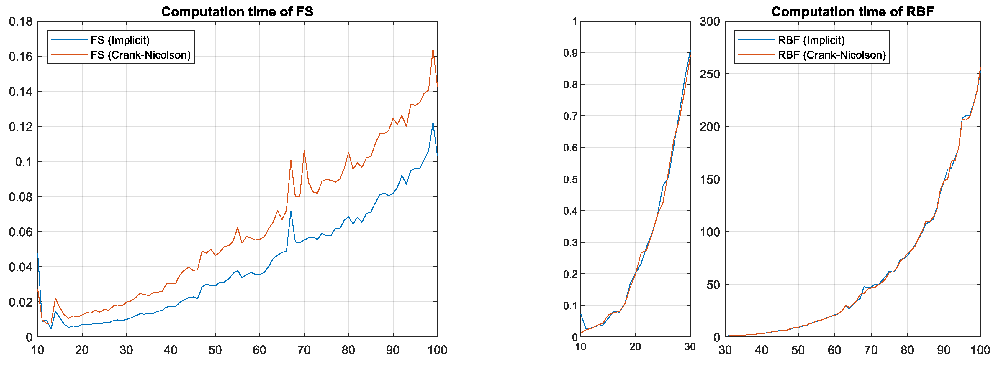
5.2. Number of Partitions of Space Dimension

The minimum number of partitions of the space dimensions is investigated to obtain accurate numerical results. Pricing errors, percentage pricing errors, and computation times are examined by changing the number of partitions of the space dimension from $M=10$ to $M=100$ with 1 increment. The decimal and percentage pricing errors are shown in Figure 1 and Figure 2, respectively. The computation times are shown in Figure 3.

Figure 1. Pricing errors (in decimals) with respect to the number of partitions of space dimensions for $\rho =-0.75$ (Left) and $\rho =0.75$ (Right), respectively.

Figure 2. Pricing errors (in percentages) with respect to the number of partitions of space dimensions for $\rho =-0.75$ (Left) and $\rho =0.75$ (Right), respectively.

Figure 3. Computation time (in seconds) with respect to the number of partitions of space dimensions for the fractional step method (FS) (Left) and the radial basis functions (RBF) (Right).

First, the results on decimal pricing errors are analyzed. The decimal pricing errors are shown in Figure 1. The pricing errors of the fractional step methods monotonically converge to zero as the number of partitions increases. The pricing errors of the radial basis functions converge to zero with fluctuations as the number of partitions increases; when the number of partitions is smaller than 50, the exchange option premium is smaller than the theoretical value for the even number of partitions, while the exchange option premium is bigger than the theoretical value for the odd number of partitions. Thus, an average of numerical value for the partition size $m$ and $m+1$ reduces pricing error. Comparing the decimal pricing errors, the fractional step method provides smaller decimal errors than the radial basis functions for a common mesh. The pricing errors for $\rho =0.75$ are greater than those for $\rho =-0.75$ when there is the same number of partitions. Option premiums are smaller for $\rho =0.75$ than for $\rho =-0.75$, which results in larger errors for $\rho =0.75$ than for $\rho =-0.75$.

Next, the results on percentage pricing errors are analyzed. The percentage pricing errors, shown in Figure 2, display similar behavior to the decimal pricing errors. The percentage pricing errors of the fractional step methods monotonically converge to zero. The percentage pricing errors of the radial basis functions converge to zero with fluctuations as the number of partitions increases. The minimum numbers of partition to achieve percentage pricing errors less than 1% are 22 and 21 for $\rho =-0.75$ applying the fractional step methods with the fully implicit scheme and the Crank–Nicolson scheme, respectively. The minimum numbers of partition size to achieve percentage pricing errors less than 1% are 45 and 54 for $\rho =0.75$ applying the fractional step methods with the fully implicit scheme and the Crank–Nicolson scheme, respectively. The minimum numbers of partition size to achieve percentage pricing errors less than 1% are 28 and 34 for $\rho =-0.75$ applying the radial basis functions with the fully implicit and the Crank–Nicolson scheme, respectively. The minimum numbers of partition size to achieve percentage pricing errors less than 1% are 66 and 78 for $\rho =0.75$ applying the radial basis functions with the fully implicit scheme and the Crank–Nicolson scheme, respectively. In conclusion, the fractional step method is more accurate than the radial basis functions when the same mesh is used.

Computation times of the fractional step method and the radial basis functions are shown in Figure 3. Here, the computation times are calculated as an average of computation times for $\rho =-0.75$ and $\rho =0.75$. The computation time of the fractional step method increases linearly as the number of partitions increases, while that of the radial basis functions grows exponentially as the number of partitions increases. Thus, when the number of partitions is 10, the computation times of the fractional step method are comparable with those of the radial basis functions; the fractional step method is much faster than the radial basis functions as the number of partitions increases. As mentioned at the end of Section 4, when the radial basis functions are conducted to evaluate exchange options, the non-negativity of option premium $f=\Phi u$ is not ensured. To recover the non-negativity of option premium, negative values of option premium at the intermediate times are replaced by zero and re-defined $u$ as $u={\Phi }^{-1}f$. This procedure takes time and increases the computation time of the radial basis functions as the number of partitions increases.

The results in this subsection confirm that both the fractional step method and the radial basis functions can appropriately solve PDEs with mixed derivative terms. Comparing their results, the fractional step method is more accurate than the radial basis functions with the same mesh and the fractional step method is much faster than the radial basis functions.

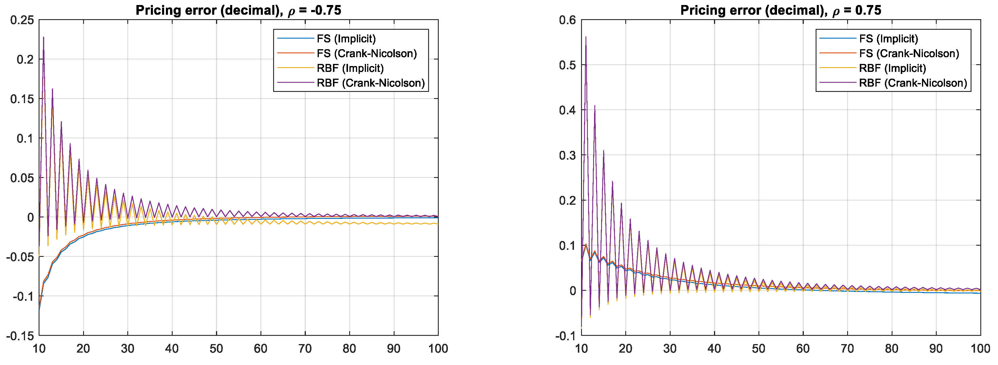
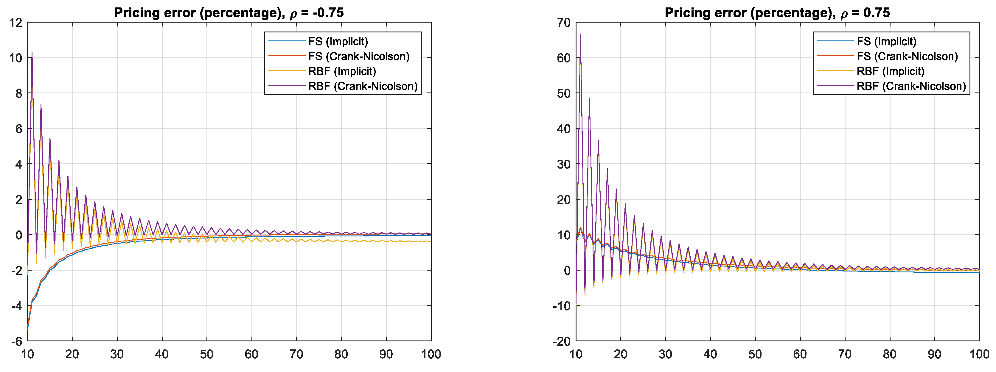
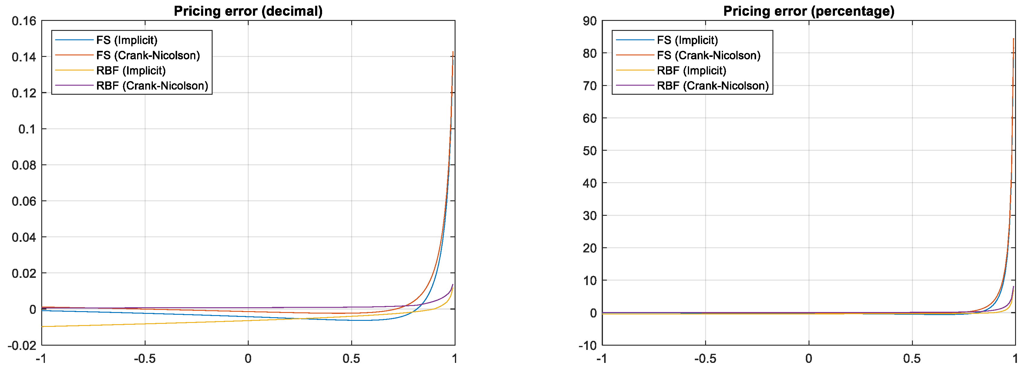
5.3. Errors with Respect to Correlation

The main purpose of this study is to examine whether the fractional step method and the radial basis functions can solve PDEs with mixed derivatives. Numerical results of exchange option premiums are obtained by changing $\rho$ from $-1$ to $0.99$ with 0.01 increments, and the results are shown in Figure 4. The exchange option premium is a decreasing function with respect to the correlation. The analytical premium varies from 2.3582 for $\rho =-1$ to 0.1692 for $\rho =0.99$.

Figure 4. Theoretical exchange option premium with respect to $\rho$.

First, the decimal pricing errors are examined with respect to the correlations, as depicted in Figure 5. The decimal pricing errors of the fractional step method using the fully implicit scheme are less than 0.01 for $-1\le \rho \le 0.88$, and those using the Crank–Nicolson scheme are less than 0.01 for $-1\le \rho \le 0.85$. The decimal pricing errors of the radial basis functions using the fully implicit scheme are less than 0.01 for $-1\le \rho \le 0.98$, and those using the Crank–Nicolson scheme are less than 0.01 for $-1\le \rho \le 0.97$. Thus, the differences between the fully implicit scheme and the Crank–Nicolson scheme are negligible for the fractional step method and for the radial basis functions. For strong correlations, the decimal and percentage pricing errors of the fractional step method are greater than those of the radial basis functions. The decimal pricing errors of the fractional step method at $\rho =0.99$ are 0.138251 and 0.142960 for the fully implicit scheme and the Crank–Nicolson scheme, respectively. The decimal pricing errors of the radial basis functions at $\rho =0.99$ are 0.01183 and 0.013793 for the fully implicit scheme and the Crank–Nicolson scheme, respectively. Thus, the radial basis functions give accurate numbers, even for an extremely strong correlation.

Figure 5. Decimal (Left) and percentage (Right) pricing errors of the fractional step method (FS) and the radial basis functions (RBF) with respect to the correlation.

Next, the percentage pricing errors are examined with respect to the correlations, shown in Figure 5. The behavior of the percentage pricing errors is similar to that of the decimal pricing errors. The percentage pricing errors of the fractional step method using the fully implicit scheme are less than 1% for $-1\le \rho \le 0.86$, and those using the Crank–Nicolson scheme are less than 1% for $-1\le \rho \le 0.82$. The percentage pricing errors of the radial basis functions using the fully implicit scheme are less than 1% for $-1\le \rho \le 0.95$, and those using the Crank–Nicolson scheme are less than 1% for $-1\le \rho \le 0.91$. Thus, the fractional step method gives sufficiently accurate results except for extremely strong correlations. The radial basis functions give more accurate results than the fractional step method with the same mesh.

The pricing errors of the fractional step method are reduced by increasing the number of partitions for time and space dimensions to $N=120$ and $M=250$, respectively. The decimal and percentage pricing errors are depicted in Figure 6. Using this mesh, the percentage errors of the fractional step method using the fully implicit scheme are less than 1% for $-1\le \rho \le 0.94$, and those using the Crank–Nicolson scheme are less than 1% for $-1\le \rho \le 0.93$. Despite the large number of partitions, the computation time is less than the radial basis functions with $N=30$ and $M=80$.

Figure 6. Percentage pricing errors of the fractional step method (FS) with a finer mesh, N = 120 and M = 250 with respect to the strong correlation.

6. Conclusions

This study conducts numerical experiments to solve PDEs with mixed derivatives. The experiments show that both the fractional step method and the radial basis functions are efficient methods to solve PDEs with mixed derivatives. The computation time of the radial basis functions is longer than that of the fractional step method when the numbers of partitions are the same. The computation time of the radial basis functions increases exponentially as the number of partitions increases. The radial basis functions do not ensure the non-negativity of the option premium, and it takes time to recover the non-negativity of the option premium at the intermediate times. The computation time of the fractional step method increases linearly as the number of partitions increases. Moreover, the fractional step method gives accurate results even with relatively small numbers of partitions. Both the fractional step method and the radial basis functions give accurate numbers except for the extremely strong correlations. Even under the extremely strong correlations, the fractional step method gives accurate results by increasing the number of partitions with computation time less than the radial basis functions. Therefore, this study concludes that the fractional step method is superior to the radial basis function.

Both numerical methods are applicable to various option pricings in two space dimensions such as equity options under stochastic interest rates, multi-factor interest rate models, credit derivatives under stochastic interest rates and default intensity, and so forth. Moreover, these methods can be applied to a PDE with more than two dimensions. We leave these problems for further research.

References

- Amin, Kaushik I., and Robert A. Jarrow. 1992. Pricing options on risky assets in a stochastic interest rate economy. Mathematical Finance 2: 217–37. [Google Scholar] [CrossRef]
- Ballestra, Luca Vincenzo, and Graziella Pacelli. 2013. Pricing European and American options with two stochastic factors: A highly efficient radial basis function approach. Journal of Economic Dynamics and Control 37: 1142–67. [Google Scholar] [CrossRef]
- Brummelhuis, Raymond, and Ron T. L. Chan. 2014. A radial basis function scheme for option pricing in exponential Lévy models. Applied Mathematical Finance 21: 238–69. [Google Scholar] [CrossRef]
- Chan, Ron Tat Lung. 2016. Adaptive radial basis function methods for pricing options under jump-diffusion models. Computational Economics 47: 623–43. [Google Scholar] [CrossRef]
- Company, Rafael, Vera N. Egorova, Lucas Jódar, and Fazlollah Soleymani. 2018. A local radial basis function method for high-dimensional American option pricing problems. Mathematical Modelling and Analysis 23: 117–38. [Google Scholar] [CrossRef]
- Duffy, Daniel J. 2006. Finite Difference Methods in Financial Engineering: A partial Differential Equation Approach. Sussex: John Wiley & Sons, Inc. [Google Scholar]
- Fasshauer, Gregory E. 2007. Meshfree Approximation Methods with Matlab. Singapore: World Scientific. [Google Scholar]
- Golbabai, Ahmad, Davood Ahmadian, and Mariyan Milev. 2012. Radial basis functions with application to finance: American put option under jump diffusion. Mathematical and Computer Modelling 55: 1354–62. [Google Scholar] [CrossRef]
- Goto, Yumi, Zhai Fei, Shen Kan, and Eisuke Kita. 2007. Options valuation by using radial basis function approximation. Engineering Analysis with Boundary Elements 31: 836–43. [Google Scholar] [CrossRef]
- Heath, David, Robert Jarrow, and Andrew Morton. 1992. Bond pricing and the term structure of interest rates: A new methodology for contingent claims valuation. Econometrica 60: 77–105. [Google Scholar] [CrossRef]
- Hendricks, Christian, Matthias Ehrhardt, and Michael Günther. 2016. High-order ADI schemes for diffusion equations with mixed derivatives in the combination technique. Applied Numerical Mathematics 101: 36–52. [Google Scholar] [CrossRef]
- Heston, Steven L. 1993. A closed-form solution for options with stochastic volatility with applications to bond and currency options. The Review of Financial Studies 6: 327–43. [Google Scholar] [CrossRef]
- Hon, Yiu-Chung, and Xian-Zhong Mao. 1998. A Radial Basis Function Method for Solving Options Pricing Model. Working paper. Hong Kong: City University of Hong Kong. [Google Scholar]
- Ikonen, Samuli, and Jari Toivane. 2007. Componentwise splitting methods for pricing American options under stochastic volatility. International Journal of Theoretical and Applied Finance 10: 331–61. [Google Scholar] [CrossRef]
- In’t Hout, K. J., and S. Foulon. 2010. ADI finite difference schemes for option pricing in the Heston model with correlation. International Journal of Numerical Analysis and Modeling 7: 303–20. [Google Scholar]
- Itkin, Andrey, and Peter Carr. 2008. A Finite-Difference Approach to the Pricing of Barrier Options in Stochastic Skew Models. Working paper. UCLA College: Los Angeles. [Google Scholar]
- Jäckel, Peter. 2002. Monte Carlo Methods in Finance. Sussex: John Wiley & Sons, Ltd. [Google Scholar]
- Jebreen, Haifa Bin. 2019. A Gaussian radial basis function-finite difference technique to simulate the HCIR equation. Journal of Computational and Applied Mathematics 347: 181–95. [Google Scholar] [CrossRef]
- Jeong, Darae, and Junseok Kim. 2013. A comparison study of ADI and operator splitting methods on option pricing models. Journal of Computational and Applied Mathematics 247: 162–71. [Google Scholar] [CrossRef]
- Kadalbajoo, Mohan K., Alpesh Kumar, and Lok Pati Tripathi. 2016. A radial basis function based implicit–explicit method for option pricing under jump-diffusion models. Applied Numerical Mathematics 110: 159–73. [Google Scholar] [CrossRef]
- Lando, David. 1998. On Cox processes and credit risky securities. Review of Derivatives Research 2: 99–120. [Google Scholar] [CrossRef]
- Liu, Gui-Rong. 2009. Meshfree Methods: Moving Beyond the Finite Element Method, 2nd ed. Boca Raton: CRC Press. [Google Scholar]
- Liu, Gui-Rong, and Yuan-Tong Gu. 2005. An Introduction to Meshfree Methods and Their Programming. Berlin: Springer. [Google Scholar]
- Lung, Ron Tat, and Chan Simon Hubbert. 2014. Options pricing under the one-dimensional jump-diffusion model using the radial basis function interpolation scheme. Review of Derivatives Research 17: 161–89. [Google Scholar]
- Margrabe, William. 1978. The value of an option to exchange one asset for another. The Journal of Finance 33: 177–86. [Google Scholar] [CrossRef]
- Mollapouras, Reza, Ali Fereshtian, and Michèle Vanmaele. 2019. Radial basis functions with partition of unity method for American options with stochastic volatility. Computational Economics 53: 259–87. [Google Scholar] [CrossRef]
- Saib, Aslam Aly El-Faïdal, Désiré Yannick Tangman, and Muddun Bhuruth. 2012. A new radial basis functions method for pricing American options under Merton’s jump-diffusion model. International Journal of Computer Mathematics 89: 1164–85. [Google Scholar] [CrossRef]
- Shcherbakov, Victor, and Elisabeth Larsson. 2016. Radial basis function partition of unity methods for pricing vanilla basket options. Computers & Mathematics with Applications 71: 185–200. [Google Scholar]
- Shreve, Steven E. 2004. Stochastic Calculus for Finance I: The Binomial Asset Pricing Model. New York: Springer. [Google Scholar]
- Toivanen, Jari. 2010. A componentwise splitting method for pricing American options under the Bates model. In Applied and Numerical Partial Differential Equations. Edited by Fitzgibbon William, Yuri Kuznetsov, Pekka Neittaanmäki, Jacques Périaux and Olivier Pironneau. New York: Springer, pp. 213–27. [Google Scholar]
- Yanenko, Nikolaj N. 1971. The Method of Fractional Steps. Berlin: Springer. [Google Scholar]