Does Time Varying Risk Premia Exist in the International Bond Market? An Empirical Evidence from Australian and French Bond Market

Abstract

The presence of risk premium is an issue that weakens the rational expectation hypothesis. This paper investigates changing behavior of time varying risk premium for holding 10 year maturity bond using a bivariate VARMA-DBEKK-AGARCH-M model. The model allows for asymmetric risk premia, causality and co-volatility spillovers jointly in the global bond markets. Empirical results show significant asymmetric partial co-volatility spillovers and risk premium exist in the bond markets. The estimates of the bivariate risk premia show bi-directional causality exist between the Australia and France Bond markets. Overall results suggest nonexistence of pure rational expectation theory in the risk premium model. This information is useful for the agents’ strategic policy decision making in global bond markets.

1. Introduction

Conditional volatility models are routinely estimated within the univariate and multivariate contexts for time varying return volatility, risk-premia, and volatility spillovers in the high-to-low frequency financial data. Since volatility is unobservable, the researchers have argued to model volatility utilizing (i) realized volatility, (ii) implied volatility, and (iii) conditional volatility in the financial markets, see McAleer et al. (2009) and Tsay (2010). Engle (1982) first explicitly developed a conditional volatility model known as autoregressive conditional heteroscedasticity (or ARCH) model. Subsequently, Bollerslev (1986) extended the ARCH of Engle (1982) to include dynamic volatility in the ARCH specification, known as the generalized ARCH (or GARCH) model. Tsay (1987) showed that the Engle’s (1982) ARCH can be derived from a first order random coefficient autoregressive process. The basic ARCH and GARCH models are popular in applied univariate economics and finance, yet they are incapable to capture asymmetric “news” that often arrives in the financial markets during the periods of asset trading and delayed transactions. Since “news” are unobservable and random, various proxies have been used in the finance literature to tackle the unobservable nature of the news variable, see Glosten et al. (1993), Ding et al. (1993), Beg and Anwar (2014) among others. As the financial volatility of returns are “news” dependent, it is of interest to create a variable that can be used as a proxy for the “news” to understand the effect of the so-called “good” and “bad” news in the financial markets in general. Within the univariate context, Glosten et al. (1993) develop a threshold type GARCH (synonym with TGARCH or GJR-GARCH or asymmetric GARCH) and Nelson (1991) developed asymmetric volatility model known as Exponential GARCH (EGARCH) model. Both the GJR and EGARCH capture news effect of volatility but their functional forms are different. Engle and Ng (1993) develop nonparametric diagnostic test that emphasize the asymmetry of volatility response to news. The conditional volatility specification of Ding et al. (1993) is called asymmetric power ARCH (or APARCH) model. The APARCH model nests both asymmetric model of Glosten et al. (1993) and EGARCH model of Nelson (1991). Another development of the univariate ARCH/GARCH model is the time varying ARCH-in-mean (or ARCH-M) model, first introduced by Engle et al. (1987). This model captures risk premium for holding risky assets.

In this paper, we employ both univariate and bivariate asymmetric GARCH-in mean (AGARCH-M) model where a conditional variance is a determinant of time-varying risk premia. Which enters in the forecast equation of the expected bond returns. Any increase in the expected return will be identified as risk premium. The presence of risk premium is an issue that weakens the rational expectation hypothesis see, Shiller (1978, 1981), Shiller et al. (1983); Campbell (1986); Engle et al. (1987) among others for the univariate case. This paper, explores linkages between Australia and France bond markets connecting two different continents using bivariate VARMA-DBEKK-AGARCH-M model. The model is estimated by the quasi-maximum likelihood (in absence of multivariate Gausinity) for the Australian and French data. The model investigates the direction of causality, co-volatility spillovers, and presence of risk premia jointly across the two markets. The existence of time varying risk premium, and asymmetric co-volatility spillovers are the most valuable sources of information through which efficient portfolio allocation and diversification can be understood across markets both locally and globally. This information is useful for measuring and predicting volatility, pricing securities, and risk management in general.

The structure of the paper is as follows. In Section 2, Review of related literature and in Section 3, Data, models and methodology are discussed. Section 4 presents empirical results. Finally, Section 5 concludes the paper.

2. Review of Related Literature

Markowitz (1959) developed a testable form of asset allocation utilizing mean-variance approach. The principles of the mean-variance lies on the following optimization rules:

• Minimize the variance of portfolio return given expected return, and
• Maximize expected return, given variance.

Motivated by the work of Markowitz (1959); Sharpe (1964) and Lintner (1965) independently developed a model of “dependence” between expected returns and risk in dealing with risk–return nexus. Sharpe (1964) and Lintner (1965), introduce their models with additional two key assumptions: (a) All investors are assumed to follow the mean variance rule, and (b) unlimited lending and borrowing at the risk–free rate, $r_f$, which does not depend on the amount borrowed or lent.

This model is known as capital asset pricing model (CAPM). The theory of CAPM states that the risk premium on a security is proportional to the risk premium on market portfolio. That is $r_i-r_f\propto \left(r_m-r_f\right)$, where $r_i$ and $r_f$ are the returns on security $i$ and the risk-free rate, respectively, $r_m$ is the return on the market portfolio, and the proportionality constant of the model is denoted by ${\beta }_i$ is the $i-$th security’s “beta” value. A stock’s beta is important to investors and policy makers since it reveals the stock’s volatility. This model has been extensively used in empirical finance. Although theoretically, the CAPM is sound but suffers from empirical evidence.

Poor empirical performance of the traditional static CAPM gives rise to modification of the CAPM. Basu (1977, 1983) gave evidence that when common stocks are sorted on earnings–price ratios (E/P), the future returns on high E/P stocks are higher than predicted by the traditional CAPM. Banz (1981) documented a size effect when stocks are sorted by market capitalization, in which average returns on small stocks are higher than predicted by the CAPM. Stattman (1980) and Rosenberg et al. (1985) documented those stocks with high book-to-market equity ratios have high average returns that are not captured by their betas. Fama and French (1992) updated and synthesized the evidence on the empirical failures of the CAPM. Using the cross-sectional regression approach, Fama and French confirm that size, earnings–price, debt–equity, and book-to-market ratios added to the explanation of expected stock returns provided by market betas. Fama and French (1996) reach the same conclusion using the time-series regression applied to portfolios of stocks sorted by price ratios.

Jagannathan and Wang (1996) included other risk factors, different from Fama and French (1992), into the model and found some support to the theory and practice of CAPM. Specifically, they found some improvements of the model for monthly data rather than annual data. The Fama and French (1992) model is known as three factor asset pricing model in finance. They further extended the model by including a few other exogenous variables into the model. The Fama and French (2015) five factor asset pricing model directed at capturing the size, value, profitability, and investment patterns in average stock returns and found that the five-factor model performs better than the three-factor model. However, the five-factor model's main problem is its failure to capture the low average returns on small stocks whose returns behave like those of firms that invest a lot despite low profitability. Ratios involving stock prices have information about expected returns missed by market betas. Such ratios are thus prime candidates to expose shortcomings of asset pricing models in the case of the CAPM, shortcomings of the prediction that market betas suffice to explain expected returns. These observations may be regarded as misspecification of the traditional CAPM due to omitted variables. So, the consequence of the traditional CAPM might suffer from bias and inconsistency.

Another important issue of the failure of empirical support to CAPM might be the linearity assumption of expected returns. The linear model could perform badly in empirical applications if the linearity assumption is violated. It is well known that most of the asset returns exhibit stylized facts, e.g., limit cycles, sudden jumps, amplitude-frequency dependencies, and nonlinearity. The inherent nonlinearity of the traditional linear CAPM could be a model specification problem. Therefore, the assumption of linearity of CAPM needs to be tested before adopting such a model for policy decision analysis. One of the sources of inherent nonlinearity may enter into the model through the conditional second moment of the financial return series. If linearity does not hold then the use of correlation as a measure of dependence between different financial assets is not appropriate for optimal portfolio selection by the CAPM. Therefore, the traditional static CAPM approach founded on the assumption of multivariate normality could not be appropriate. This may be regarded as functional misspecification of the traditional CAPM.

The nonlinearity that may enter into the returns series was first cleverly modelled by the Nobel Laureate Robert Engle in 1982. This model is known as autoregressive conditional heteroskedastic (ARCH) model, widely used in the finance and elsewhere. Engle showed that it is possible to model the conditional mean and conditional variance of a series of observations jointly. This theory is a stronger additional contribution to the traditional static CAPM. The ARCH model captures various stylized facts that exhibited by the financial asset returns, such as volatility clustering, asymmetry, and a high degree of persistence. Bollerslev (1986) extended Engles’s (1982) ARCH by developing a technique that allows the conditional variance to be an autoregressive moving average (ARMA) process. This expanded conditional variance is widely known as Generalized Autoregressive Conditional Heteroskedastic (GARCH) model, Bollerslev (1986). These two models are widely used in empirical finance for volatility modelling.

Although the ARCH/GARCH models are popular and extensively used in finance literature, however they are restricted only to symmetric information. Various extensions of ARCH/GARCH has appeared in the literature to overcome some inherent nonlinearity problems within GARCH class of models. Since volatility clustering is the likely characteristic of financial returns which is nonlinear by nature, can be modelled by asymmetric t-distribution, generalized error distribution, extreme-value theory among others. A popular nonlinear extension of ARCH/GARCH is the Nelson’s (1991) exponential generalized autoregressive conditional hetroscedasticity (EGARCH) model. It attempted to include asymmetric impact of shocks on volatility. In addition, this model does not require the non-negativity restrictions on the parameters contradictory to ARCH/GARCH conditional volatility models.

Another popular extension of GARCH is the Glosten et al. (1993) is known as GJR-return volatility model in financial econometrics. Other asymmetric models include “News impact curves” of Engle and Ng (1993), nonlinear asymmetric GARCH (NAGARCH) and vector AGARCH (VAGARCH) of Engle (1990) among others. These models have different centers than the EGARCH and GJR. It is important to note that if a negative return shock causes more volatility than a positive shock of the same size, the classical GARCH model under predicts the amount of volatility following bad news and over predicts the amount of volatility following good news.

The asset pricing theories agree that a high risk has to be compensated by higher expected returns. It is therefore, reasonable to include variance into the expected return model to take account of risk premium. The resulting model is known as ARCH-in-Mean (ARCH-M) model and GARCH-in-Mean (GARCH-M) models within the ARCH/GARCH context. ARCH-M model was first introduced by Engle et al. (1987) in the univariate context. Significance of the ARCH-M could be treated as a failure of efficient market hypothesis (EMH) represented by the traditional CAPM. Bollerslev et al. (1988) address the issue of risk premia within the multivariate GARCH-M framework. Their result support the time-varying conditional variance–covariance of the asset returns. They also found significant risk premia influenced by the conditional moment results. On the issue of risk premium, Christoffersen et al. (2012) derived the distribution of returns using a two-factor volatility model, namely dynamic volatility and dynamic jump intensity. In their model each factor ties own risk premium. Using U.S. returns, they find statistically significant results which outperform the standard model without the jumps. They found significant risk premium on the dynamic jump intensity which has a much larger impact on option prices. Combining the jump diffusion and GARCH, Arshanapalli et al. (2011) tested the risk–return relationship in the U.S. stock returns. They found significant relationship between the risk and the return.

Campbell et al. (2020), generates time-varying risk premia on bonds and stocks based on consumption-based habit model of homoskedastic macroeconomic dynamics. They found co-movement of macroeconomic dynamics of stocks and bonds return. This information could help modelling time-varying risk premia in a wide range of consumption-based risk premium. Cochrane and Piazzesi (2005) studied time variation in expected excess bond returns. They focus on real risk premia in the real term structure. Their multiple regression of excess returns on all forward rates provide stronger evidence against expectations hypothesis. Which indicates that a single linear combination of forward rates forecasts returns of all maturities. They do not include the time-varying premium to macroeconomic or monetary fundaments in the model.

3. The Data, Models and Methodology

3.1. The Data

The 10 year maturity bond price series for the Australia and France markets are extracted from The Bloomberg database. The series starts at 4 January 1990 and the sample period ends on 30 December 2016. The daily bond return having maturity of ten year is constructed using

r_t = 100 * ln (p_t/p_t−1)

(1)

where $p_t$ is the bond price at time t and $p_{t-1}$ is the one period lag series. The $r_t$ in (1) is called the continuously compounded return or log return in percentage.

Empirical analysis begins with numerical descriptive statistics and graphical means of observing the properties of for the Australian and French bond returns data. We then perform the unit root tests followed by diagnostic tests for the return series to examine the statistical properties in Section 4. We report the quasi-maximum likelihood estimates (QMLEs) in absence of Gaussinity of the standardized return shock of the univariate autoregressive moving average asymmetric GARCH in mean (ARMA-AGARCH-M) models followed by the multivariate estimation of the two country’s vector autoregressive moving average diagonal BEKK—asymmetric GARCH-M (VARMA-DBEKK-AGARCH-M) model. The Granger causality of the bond returns, and the partial co-volatility spillovers for the bivariate bond returns investigated.

3.2. Specification of the Model

To understand the dynamic interdependence of bond returns, time-varying risk-premium, causality, and co-volatility spillovers, we utilize VARMA-DBEKK-AGARCH-M model. This model nests a wide range of multivariate volatility models and considers various issues of modelling real financial series. This model is capable to extract asymmetry, Granger-type causality and Chang et al. (2018) type co-volatility spillovers between assets across countries.

3.2.1. Univariate Models for Conditional Mean and Conditional Volatility

For the conditional mean of security return, r_t, we use Box–Jenkin’s autoregressive moving average (ARMA) model as follows.

$$r_t|F_{t-1}={\varphi }_0+{{\displaystyle \sum }}_{j=1}^k{\varphi }_j{r}_{t-j}+{{\displaystyle \sum }}_{l=1}^m{\psi }_l{\epsilon }_{t-l}+{\epsilon }_t$$

(2)

where ${\varphi }_o,{\varphi }_j, {\psi }_l$ are scalar parameters of the ARMA($k,m$) process, ${\epsilon }_t$ is the innovation or return shock, $F_{t-1}$ is the set of information available at time $t$. The AIC and BIC are routinely used in empirical applications for ARMA order selection. A benchmark model for volatility proposed by Bollerslev (1986) called generalized autoregressive conditional heteroskedasticity (GARCH) model, which takes the following form.

GARCH(p, q):

$$E({\epsilon }_t^2|F_{t-1})=h_t=w+{{\displaystyle \sum }}_{j=1}^q{\alpha }_j{\epsilon }_{t-j}^2+{{\displaystyle \sum }}_{l=1}^p{\beta }_l{h}_{t-l}$$

(3)

The order of GARCH q = 1 and p = 1 has been found appropriate in real applications, Bollerslev (1986, 1987).

The GARCH is a generalization of Engle (1982) autoregressive conditional heteroskedastic (ARCH) model. The basic ARCH/GARCH model cannot distinguish between the asymmetric shocks on volatility, which is a common phenomenon of financial return series. Glosten et al. (1993) (or GJR) develop a model which accounts for asymmetric volatility called AGARCH, takes the following form.

$$\begin{array}{c}{h}_t|F_{t-1}=w+{{\displaystyle \sum }}_{l=1}^p{\beta }_l{h}_{t-l}+{{\displaystyle \sum }}_{j=1}^q{\alpha }_{jl}{\epsilon }_{t-l}^2+{{\displaystyle \sum }}_{l=j}^p{\gamma }_j{d}_{t-j}{\epsilon }_{t-j}^2,\mathrm{where}\\ d_{t-j}=\{\begin{array}{c}1 if{\epsilon }_{t-j}<0\\ 0 otherwise\end{array}\end{array}$$

(4)

Engle et al. (1987), allows the conditional mean returns to depend on its own conditional variance. This model is suitable for analysis of the asset markets’ time varying risk premiums with intent to consider situations where the risk-averse agents require compensation for holding risky assets. This model is generally known as risk premium model expressed as follows.

$$r_t={\mu }_t+{\delta }_{}g\left(h_t\right)+{\epsilon }_t$$

(5)

where ${\mu }_t$ is the conditional mean generated by model (2), $h_t$ is as defined in (3). In finance, $\delta g\left(h_t\right)$ represent the risk premium, see Bera and Higgins (1993). In most applications $g\left(h_t\right)=\sqrt{h_t}$ has been used, for example, Domowitz and Hakkio (1985) and Bollerslev et al. (1988). The GJR specification for conditional volatility when added in the asset return equation, the resulting model (5) becomes GJR-GARCH-M.

3.2.2. Multivariate Models for Conditional Mean and Conditional Volatility

Let $r_t=\left(r_{1t},r_{2t},\dots \dots .,r_{Nt}\right){}^{\prime }$ be an ($N\times 1$) vector of $N$-dimensional asset returns or log returns at the time index $t=1,2,\dots \dots ,T$ with the following structure.

$$r_t|F_{t-1}={\mu }_t+{\epsilon }_t,{\epsilon }_t=H^{0.5}{e}_t$$

(6)

where ${\mu }_t=E(r_t|F_{t-1})$ is the conditional expectation of the vector $r_t$ given the past information $F_{t-1}$ and ${\epsilon }_t=\left({\epsilon }_{1t},{\epsilon }_{2t},\dots \dots .,{\epsilon }_{Nt}\right){}^{\prime }$ is an $\left(N\times 1\right)$ vector of shocks, or innovation at time $t$. Each component of $r_t$ vector is a univariate return of an asset. The $e_t$=$e_{1t},e_{2t},\dots \dots ,e_{Nt}$ is an ($N\times 1$) vector of $\mathit{i.i.d.}$ random vector with probability distribution, say, $G\left(0,I_N\right)$, where $G$ is assumed to be a continuous, $I_N$ is the identity covariance matrix, and 0 is an $N\times 1$ mean vector. The multivariate conditional return can be expressed as a vector autoregressive moving average (VARMA) model as follows.

$$r_t={\mathsf{\Phi }}_0+{{\displaystyle \sum }}_{i=1}^k{\mathsf{\Phi }}_i{r}_{t-i}+{{\displaystyle \sum }}_{l=1}^m{\mathsf{\Psi }}_l{\epsilon }_{t-l}+{\epsilon }_t$$

(7)

where ${\mathsf{\Phi }}_0$ is a $\left(N\times 1\right)$ vector of intercept, ${\mathsf{\Phi }}_i$ and ${\mathsf{\Psi }}_l$ are both ($N\times N$) matrices for each i and l of various lags. The vector of returns can be tested for stationarity. The $\left(N\times N\right)$ covariance matrix $H_t$ with component $h_{ijt},\left(i,j=1,2,\dots \dots N\right),$ need to be specified. Various forms of $H_t$ have been proposed, for example, Silvennoinen and Teräsvirta (2009), Bauwens et al. (2006), Tsay (2006). The two most popular multivariate conditional volatility specifications are the Bollerslev et al. (1988) VEC and Engle and Kroner (1995) BEKK specifications. In the present paper we focus on a diagonal variant of BEKK.

3.2.3. VARMA-DBEKK-AGARCH-in Mean Model

We consider the following form of the multivariate risk premia model.

Return:

$$r_t|F_{t-1}={\mathsf{\Phi }}_0+{{\displaystyle \sum }}_{i=1}^k{\mathsf{\Phi }}_i{r}_{t-i}+{{\displaystyle \sum }}_{l=1}^m{\mathsf{\Psi }}_l{\epsilon }_{t-l}+\delta H_t^{1/2}+{\epsilon }_t$$

(8)

DBEKK-AGARCH:

$$H_t|F_{t-1}=C{}^{\prime }C+{{\displaystyle \sum }}_{j=1}^q{A}_j\left({\epsilon }_{t-j}{\epsilon }_{t-j}^{{}^{\prime }}\right)A{}^{\prime }+{{\displaystyle \sum }}_{l=1}^p{B}_l{H}_{t-l}{B}_l^{{}^{\prime }}+{{\displaystyle \sum }}_{j=1}^q{\Gamma }_j\left(D_{jt}\times \left({\epsilon }_{t-j}{\epsilon }_{t-j}^{{}^{\prime }}\right){\Gamma }_j^{{}^{\prime }}\right)$$

(9)

In model (8) the conditional expected return is augmented by the function of conditional volatility model (9). In the above model (9), the matrices $A$, $B$, and $\Gamma$ are assumed to be diagonal. The matrix $C$ is a lower triangular matrix. A simpler version of (9) with $p=1 \mathrm{and} q=1$, takes the following form.

$$H_t|F_{t-1}=C{}^{\prime }C+A\left({\epsilon }_{t-1}{\epsilon }_{t-1}^{{}^{\prime }}\right)A{}^{\prime }+B_l{H}_{t-1}B{}^{\prime }+\Gamma (D_{t-1}\times \left({\epsilon }_{t-1}{\epsilon }_{t-1}^{{}^{\prime }}\right)\Gamma {}^{\prime }$$

(10)

where

$$D_{t-1}=\{\begin{array}{c}1 if{\epsilon }_{t-1}<0\\ 0 if{\epsilon }_{t-1}\le 0\end{array}$$

the other variables are as defined above. Let us assume that ${\epsilon }_t=H_t{\eta }_t$, where ${\eta }_t$ is a vector of identically and independently distributed vector of random variables with mean zero vector and unit variance covariance matrix.

3.3. Estimation

The estimators of the parameters of the models (8) and (9) are obtained by maximizing the log likelihood function

$$L\left(\theta \right)=\left(\frac{1}{T}\right){{\displaystyle \sum }}_{t=1}^T{l}_t\left(\theta \right)$$

(11)

$$\mathrm{where}{l}_t\left(\theta \right)=-0.5{{\displaystyle \sum }}_t\left(\mathit{ln}|H_t|+{\epsilon }_t{H}_t^{-1}{\epsilon }_t^{{}^{\prime }}\right)$$

where $\theta$ is the set of parameters of the models (8) and (9), $l_t\left(\theta \right)$ is the log of the argument, |.| is the determinant of the argument. Equation (11) takes the form of the Gaussian likelihood. Because we do not assume multivariate normality of the standardized return shock ${\eta }_t$, estimators of the parameters from (11) are the quasi-maximum likelihood estimators (QMLEs). The QMLEs are consistent and asymptotically normal, see Ling and McAleer (2003), Chang et al. (2018). Therefore, the classical asymptotic tests are valid for statistical inference.

3.4. Co-Volatility Spillovers Effect

Volatility spillover effects can be estimated utilizing the definitions given in the paper by Chang et al. (2017, 2018). In this paper, we apply the partial co-volatility spillovers as follows:

$$\frac{\partial H_{ijt}}{\partial {\epsilon }_{k,t-1}},i\ne j,k=\mathrm{either} i \mathrm{or} j$$

(12)

4. Empirical Results

4.1. Preliminary Data Analysis

In this section we provide both numerical and graphical descriptive analysis of the 10 year bond rates of Australia and France, and time series properties of the series for 6144 daily observations.

Table 1 below provides the basic descriptive statistics of the Australia and France bond return series each comprising 6144 observations.

Table 1. Descriptive statistics for the Daily 10-year bond returns.

Statistics	Australia	France
Mean	−0.015006 (0.4072)	−0.0031 (0.8938)
Standard deviation (st.dev)	1.4191	1.8012
Minimum	−10.7556	−15.7247
Maximum	12.9630	20.8273
Skewness	0.295699 (0.0000)	0.3952 (0.0000)
Excess Kurtosis	5.2828 (0.0000)	7.5076 (0.0000)
Jarque and Bera (JB)	7232.9308 (0.0000)	14,586.7843 (0.0000)
Sample size	6144	6144

Note: 1. The returns are in percentages and the sample period starts 4 January 1990 and ends 30 December 2016. The data source is given in the text. 2. The p-value of the test is in parentheses.

The basic statistics of the two series show excess kurtosis, implying that the series have fat tails. Both the series are non-normal by the Jarque and Bera (1987) test. Time plot of the price and return volatility of each series shown in Figure 1a,b below.

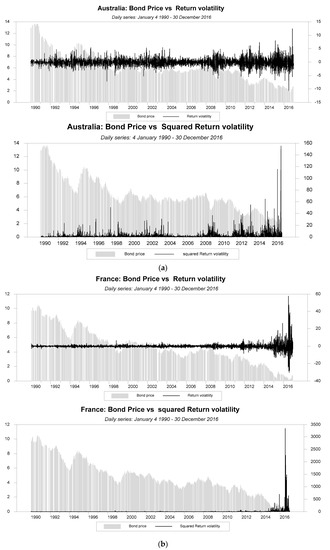
Figure 1. (a) Plot of Bond price, return volatility and squared return series of Australia; (b) Plot of Bond price, return volatility and squared return series of France.

From the Figure 1a,b above, we observe that the pattern of movement of the bond prices sloping downward for both Australia and France. However, the volatility of returns changes with varying degree of clustering across the two bond markets. The Australian bond market experience tranquil period from 2005 to 2007. However, bond return volatility started fluctuating from late 2007 until the beginning of 2010. Bond market of France on the other hand exhibit tranquility before 2007. The bond market of France increased slightly during 2008 and continue to fluctuate at a faster rate and peaked quite high during 2015 to 2016 compared with 2010. This could be due to the global and European financial crises and Russian financial crisis. The Australian bond return volatility was comparatively high during 1996 to 2004 than the previous years. This could be due to the Asian crises. While during 2008 to 2016 the volatility clustering was relatively high compared with the periods 2007. Both the markets peaked up high volatility during the global financial crisis.

Next, we utilize augmented Dickey–Fuller (ADF), Phillips–Perron (PP) and KPSS tests for stationarity property of both the Australia and France series.

The Unit root tests result of Table 2 suggests that both the bond returns series are stationary by the augmented Dickey–Fuller (ADF), Phillips–Perron (PP), and Kwiatkowski–Phillips–Schmidt–Shin (KPSS) tests. Finally, the independent, identical distribution (iid) issue of the data property is tested by the Ljung and Box (1978) [$LB$] test and the nonlinearity test of the series is conducted by the McLeod and Li (1983) Chi-square test and by the Tsay (1986)’s original-F-test (Ori-F). The test results are provided in Table 3 below.

Table 2. Unit root tests for the Bond returns.

Bond Returns	Type	Null Hypothesis	Alternative Hypothesis	Test Statistic	Critical Value
					(1% Level)	(5% Level)
Australia	ADF	Nonstationary	Stationary	−36.5301 ***	−3.435	−2.863
	PP	Nonstationary	Stationary	−84.5055 ***	−3.435	−2.863
	KPSS	Stationary	Nonstationary	0.0460	0.739	0.347
France	ADF	Nonstationary	Stationary	−37.7938 ***	−3.435	−2.863
	PP	Nonstationary	Stationary	−81.2682 ***	−3.435	−2.863
	KPSS	Stationary	Nonstationary	0.0466	0.739	0.347

Note: ‘***’ 1% significance level.

Table 3. Preliminary diagnostics tests on the return and squared return series.

Type	Australia	France
Ljung–Box$\left(LB\right)-Q\left(10\right)$	43.661 (0.000)	25.704 (0.004)
Ljung–Box$\left(LB\right)-Q\left(20\right)$	58.920 (0.000)	37.804 (0.009)
Ljung–Box$\left(LB\right)-Q^2\left(10\right)$	669.249 (0.000)	1133.363 (0.000)
Ljung–Box$\left(LB\right)-Q^2\left(20\right)$	1049.775 (0.000)	2011.404 (0.000)
McLeod–Li(10)	668.992 (0.000)	1132.953 (0.000)
McLeod–Li(20)	1048.742 (0.000)	2010.004 (0.000)
Tsay Ori_F(10, 6134) lags(4)	4.362 (0.000)	3.099 (0.001)
ARCH-LM lags(4)	68.156 (0.000)	77.092 (0.000)

Note: The p-value is in parentheses.

Serial independence of the series is rejected by the LB-tests. The series are found to be asymmetric with heavy tails by the skewness and kurtosis tests respectively. Both the series are found to be nonlinear by the McLeod and Tsay tests.

4.2. Empirical Estimation of the Univariate ARMA-AGARCH-M Models

In this section, we report the quasi-maximum likelihood estimates (QMLEs) of the univariate ARMA-AGARCH-M models for the bond return of Australia and France

(a)

Empirical estimation of risk premium of the Australia bond return having maturity of 10 year:

$$\begin{array}{c}Aus{t}_t=-{0.0451}^{***}+{0.3182}^{***}Aus{t}_{t-1}-{0.3845}^{***}{\epsilon }_{1,}{}_{t-1}+{0.01959}^{**}{h}_{1t}^{\frac{1}{2}}+{\epsilon }_{1,t}\\ \left(s.e\right) \left(0.0131\right) \left(0.0132\right) \left(0.1253\right) \left(0.0188\right)\\ h_{1t}|F_{t-1}={0.0058}^{***}+{0.025}^{***}{\epsilon }_{t-1}^2+{0.9615}^{***}{h}_{1,t-1}+{0.0221}^{***}{d}_{1t-1}{\epsilon }_{1t-1}^2\\ \left(s.e\right) \left(0.0015\right) \left(0.0038\right) \left(0.00034\right) \left(0.0221\right)\end{array}$$

where $d_{1t-1}$ is an indicator variable as defined in the text. Note: “***” significant at the 1% level; “**” significant at the 5% level.

The estimated coefficients of the Australia risk-premium model are all significant at one percent level. The risk premium parameter and the asymmetric news effect are significant. The leverage effects are found to be significant. The Ljung and Box (1978) test results on the standardized residuals and those of squared standardized residuals indicate no model inadequacy. The bond return model captures both news effect and risk premium. This information is useful for prediction of volatility and risk premium in the Australian market independently of the French market.

(b)

Empirical estimation of risk premium of the France bond return having maturity of 10 year:

$$\begin{array}{c}Franc{e}_t=-{0.0726}^{***}+0.3315Franc{e}_{t-1}-0.3504{\epsilon }_{2t-1}+{0.0145}^{**}{h}_t^{\frac{1}{2}}+{\epsilon }_{2t}\\ \left(s.e\right) \left(0.0217\right) \left(0.2911\right) \left(0.2883\right) \left(0.0058\right)\\ h_{2t}|F_{t-1}={0.0047}^{***}+{0.0340}^{***}{\epsilon }_{2t-1}^2+{0.9452}^{***}{h}_{2t-1}+{0.04361}^{***}{d}_{2t-1}{\epsilon }_{2t-1}^2\\ \left(s.e\right) \left(0.0015\right) \left(0.0048\right) \left(0.0039\right) \left(0.0063\right)\end{array}$$

where $d_{2t-1}$ is an indicator variable as defined in the text. Note: “***” significant at the 1% level; “**” significant ant the 5% level.

The Ljung and Box (1978) test result on the standardized residuals and those of squared standardized residuals indicate no model inadequacy for French data. The estimated France Bond returns indicate that the autoregressive and the moving average terms are insignificant in the model. The Univariate volatility model for France shows significant asymmetric news effect on volatility and existence of risk premium term at 5% level.

Ljung and Box (1978) test on the standardized residuals & squared standardized residuals of Australian and France risk Premium model are reported in Table 4.

Table 4. Preliminary diagnostics tests on the residuals and squared residuals of the risk premium model for Australia and France.

Type	Australia	France
$\mathrm{LB}-\mathrm{Q}\left(10\right)$	$3.759\left(0.9576\right)$	$12.550\left(0.2499\right)$
$\mathrm{LB}-{\mathrm{Q}}^2\left(10\right)$	$8.740\left(0.5569\right)$	$11.493\left(0.3204\right)$
$\mathrm{LB}-\mathrm{Q}\left(20\right)$	$13.591\left(0.8506\right)$	$31.695\left(0.047\right)$
$\mathrm{LB}-{\mathrm{Q}}^2\left(20\right)$	$16.554\left(0.6817\right)$	$20.442\left(0.4306\right)$
Log-likelihood	−10,099.3285	−9976.8864

Note: The p-value is in parentheses; Ljung–Box ($LB$).

4.3. Empirical Estimation, Causality, and Partial Co-Volatility of the VARMA-DBEKK-AGARCH-M Model

In this section we provide bi-variate estimation of the VARMA-DBEKK-AGARCH-M model

(a)

Estimation of the bivariate VARMA-DBEKK-AGARCH model.

$\left(\begin{array}{l}Aus{t}_t\\ Franc{e}_t\end{array}\right)=\left(\begin{array}{l}-0.0579***\\ \left(0.0177\right)\\ -0.0237**\\ \left(0.0103\right)\end{array}\right)+\left(\begin{array}{l}0.02100.2136***\\ \left(0.0417\right)\left(0.0101\right)\\ 0.0424***0.6064***\\ \left(0.0104\right)\left(0.1177\right)\end{array}\right)\left(\begin{array}{l}Aus{t}_{t-1}\\ Franc{e}_{t-1}\end{array}\right)+\left(\begin{array}{l}-0.1662***0\\ \left(0.0447\right)\\ 00.6381\\ \left(0.1143\right)\end{array}\right)\left(\begin{array}{l}{\epsilon }_{1t-1}\\ {\epsilon }_{2t-1}\end{array}\right)+$ $\left(\begin{array}{l}0.0433***-0.0419\\ \left(0.0162\right)\left(0.0281\right)\\ \mathrm{0.01490.0036}*\\ \left(0.213\right)\left(0.0019\right)\end{array}\right)\left(\begin{array}{l}\sqrt{h_{11}}\\ \sqrt{h_{22}}\end{array}\right)$

The estimates of the bivariate risk premia show significant causality running from France to Australia bond market and vice versa. This implies bi-directional causality exits between Australia and France Bond markets. Highly significant risk premium exists in the Australian Bond. While, weaker risk premium exists in the French Bond market compared to Australia Bond market. This could be due to the French bond market structure and financial crisis.

(b)

Empirical estimation and partial co-volatility of the DBEKK-AGARCH model

$C=\left(\begin{array}{l}0.0824***0\\ \left(0.0093\right)\\ 0.0361***-0.0652***\\ \left(0.0092\right)\left(0.0084\right)\end{array}\right),A=\left(\begin{array}{l}0.1934***\\ \left(0.0089\right)\\ 0.1352***\\ (0.0121\end{array}\right),B=\left(\begin{array}{l}0.9793***\\ \left(0.0019\right)\\ 0.9766***\\ \left(0.0018\right)\end{array}\right)$ $\Gamma =\left(\begin{array}{l}0.0417**\\ \left(0.0185\right)\\ 0.2352***\\ \left(0.0118\right)\end{array}\right)$

CNote 1. “***” indicate 1% level of significance, “**” indicate 5% level of significance, “*” indicate 10% level of significance. Note2. Standard error is in parentheses.

The partial co-volatility effects computed are as follows.

$$\begin{array}{c}\frac{\partial H_{ijt}}{\partial {\epsilon }_{k,t-1}},i\ne j\left(France,Aust\right),k=either Franceor or Australia\\ \frac{\partial H_{Aust,France,t}}{\partial {\epsilon }_{France,t}}={\stackrel{⌢}{a}}_{11}{\stackrel{⌢}{a}}_{22}{\stackrel{⌢}{\epsilon }}_{Aust,t-1}+{\stackrel{⌢}{\gamma }}_{11}{\stackrel{⌢}{\gamma }}_{22}{d}_t{\stackrel{⌢}{\epsilon }}_{Aust,t-1}=-0.00169\\ \frac{\partial H_{Aust,France,t}}{\partial {\epsilon }_{Aust,t}}={\stackrel{⌢}{a}}_{11}{\stackrel{⌢}{a}}_{22}{\stackrel{⌢}{\epsilon }}_{France,t-1}+{\stackrel{⌢}{\gamma }}_{11}{\stackrel{⌢}{\gamma }}_{22}{d}_t{\stackrel{⌢}{\epsilon }}_{France,t-1}=-0.00271\end{array}$$

where d_t is the indicator variable as defined in the text and the co-volatility spillovers from i to j computed at the average return shock.

From the above empirical results, we observe that the return volatility shocks are significant for both the bond markets. Significant asymmetry exists in both the French and Australian bond markets. The partial co-volatility shows French bond return shock negatively spillover to average co-volatility of Australian bond and French bond. It is to be noted that the Australian bond return shock negatively spillover to average co-volatility of Australian bond and French bond. The negative sign effect of return shock is an important issue in the financial asset market trading.

5. Conclusions

This paper examined volatility dynamics of the bond markets within multivariate context. This study examined the 10-year maturity of the government bond markets of Australia and France. These markets are taken in consideration for analysis because of the reason France GDP is double in size to Australia while growth rate of GDP of Australia is double and both share prime locations and are center of attractions for investors as both of those markets are well developed and matured. The VARMA-DBEKK-AGARCH-M model nests a few variants of multivariate return volatility models. The parameters of the multivariate model are estimated by the quasi-maximum likelihood method. The estimates of the bivariate VARMA-DBEKK-AGARCH-M model show significant causality running from France to Australia bond market and vice versa. This implies bi-directional causality exits between Australia and France Bond markets. The results, however, suggest nonexistence of pure rational expectation theory in the two bond markets. This information is useful particularly, for the agents’ strategic policy decision purposes in the global bond markets. For the Australian case, the estimated coefficients of the univariate ARMA-AGARCH-M are all significant at the conventional level. Significant risk-premium and leverage effect exist in the Australian long term bond. However, for France series both the AR and MA coefficients are insignificant implying that the mean model for France is constant apart from the risk premium term. This finding is useful from the investors’ point of view. One important finding is that there exist co-volatility spillovers between the two bond markets and, the Australian bond return shock negatively spillovers to average co-volatility of Australian bond and French bond and vice versa. The methodology of this paper can be applied to other global financial markets jointly, which is in our future research agenda.

References

- Arshanapalli, Bala, Frank J. Fabozzi, and William Nelson. 2011. Modeling the Time-Varying Risk Premium Using a Mixed GARCH and Jump Diffusion Model. SSRN Electronic Journal. [Google Scholar] [CrossRef]
- Banz, Rolf W. 1981. The Relationship between Return and Market Value of Common Stocks. Journal of Financial Economics. [Google Scholar] [CrossRef]
- Basu, S. 1977. Investment Performance of Common Stocks in Relation to Their Price-Earnings Ratios: A Test of the Efficient Market Hypothesis. The Journal of Finance. [Google Scholar] [CrossRef]
- Basu, Sanjoy. 1983. The Relationship Between Earnings Yeild, Market Value and Retrun for NYSE Common Stocks. Journal of Financial Economics 12: 129–56. [Google Scholar] [CrossRef]
- Bauwens, Luc, Sébastien Laurent, and Jeroen V. K. Rombouts. 2006. Multivariate GARCH Models: A Survey. Journal of Applied Econometrics. [Google Scholar] [CrossRef]
- Beg, A. B. M. Rabiul Alam, and Sajid Anwar. 2014. Detecting Volatility Persistence in GARCH Models in the Presence of the Leverage Effect. Quantitative Finance 14: 2205–13. [Google Scholar] [CrossRef]
- Bera, Anil K., and Matthew L. Higgins. 1993. ARCH MODELS: PROPERTIES, ESTIMATION AND TESTING. Journal of Economic Surveys. [Google Scholar] [CrossRef]
- Bollerslev, Tim. 1986. Generalized Autoregressive Conditional Heteroskedasticity. Journal of Econometrics. [Google Scholar] [CrossRef]
- Bollerslev, Tim. 1987. A Conditionally Heteroskedastic Time Series Model for Speculative Prices and Rates of Return. The Review of Economics and Statistics. [Google Scholar] [CrossRef]
- Bollerslev, Tim, Robert F. Engle, and Jeffrey M. Wooldridge. 1988. A Capital Asset Pricing Model with Time-Varying Covariances. Journal of Political Economy. [Google Scholar] [CrossRef]
- Campbell, John Y. 1986. Bond and Stock Returns in a Simple Exchange Model. Quarterly Journal of Economics. [Google Scholar] [CrossRef]
- Campbell, John Y., Carolin Pflueger, and Luis M. Viceira. 2020. Macroeconomic Drivers of Bond and Equity Risks. Journal of Political Economy. [Google Scholar] [CrossRef]
- Chang, Chia Lin, Michael McAleer, and Guangdong Zuo. 2017. Volatility Spillovers and Causality of Carbon Emissions, Oil and Coal Spot and Futures for the EU and USA. Sustainability (Switzerland). [Google Scholar] [CrossRef]
- Chang, Chia Lin, Michael McAleer, and Yu Ann Wang. 2018. Modelling Volatility Spillovers for Bio-Ethanol, Sugarcane and Corn Spot and Futures Prices. Renewable and Sustainable Energy Reviews. [Google Scholar] [CrossRef]
- Christoffersen, Peter, Kris Jacobs, and Chayawat Ornthanalai. 2012. Dynamic Jump Intensities and Risk Premiums: Evidence from S&P500 Returns and Options. Journal of Financial Economics. [Google Scholar] [CrossRef]
- Cochrane, John H., and Monika Piazzesi. 2005. Bond Risk Premia. American Economic Review. [Google Scholar] [CrossRef]
- Ding, Zhuanxin, Clive W. J. Granger, and Robert F. Engle. 1993. A Long Memory Property of Stock Market Returns and a New Model. Journal of Empirical Finance. [Google Scholar] [CrossRef]
- Domowitz, Ian, and Craig S. Hakkio. 1985. Conditional Variance and the Risk Premium in the Foreign Exchange Market. Journal of International Economics. [Google Scholar] [CrossRef]
- Engle, Robert F. 1982. Autoregressive Conditional Heteroscedasticity with Estimates of the Variance of United Kingdom Inflation. Econometrica. [Google Scholar] [CrossRef]
- Engle, Robert F. 1990. Stock Volatility and the Crash of ’87: Discussion. The Review of Financial Studies 3: 103–6. [Google Scholar] [CrossRef]
- Engle, Robert F., and Kenneth F. Kroner. 1995. Multivariate Simultaneous Generalized Arch. Econometric Theory. [Google Scholar] [CrossRef]
- Engle, Robert F., and Victor K. Ng. 1993. Measuring and Testing the Impact of News on Volatility. The Journal of Finance. [Google Scholar] [CrossRef]
- Engle, Robert F., David M. Lilien, and Russell P. Robins. 1987. Estimating Time Varying Risk Premia in the Term Structure: The Arch-M Model. Econometric. [Google Scholar] [CrossRef]
- Fama, Eugene F., and Kenneth R. French. 1992. The Cross-Section of Expected Stock Returns. The Journal of Finance. [Google Scholar] [CrossRef]
- Fama, Eugene F., and Kenneth R. French. 1996. Multifactor Explanations of Asset Pricing Anomalies. The Journal of Finance. [Google Scholar] [CrossRef]
- Fama, Eugene F., and Kenneth R. French. 2015. A Five-Factor Asset Pricing Model. Journal of Financial Economics. [Google Scholar] [CrossRef]
- Glosten, Lawrence R., Ravi Jagannathan, and David E. Runkle. 1993. On the Relation between the Expected Value and the Volatility of the Nominal Excess Return on Stocks. The Journal of Finance. [Google Scholar] [CrossRef]
- Jagannathan, Ravi, and Zhenyu Wang. 1996. The Conditional CAPM and the Cross-Section of Expected Returns. The Journal of Finance. [Google Scholar] [CrossRef]
- Jarque, Carlos M., and Anil K. Bera. 1987. A Test for Normality of Observations and Regression Residuals. International Statistical Review / Revue Internationale de Statistique. [Google Scholar] [CrossRef]
- Ling, Shiqing, and Michael McAleer. 2003. On Adaptive Estimation in Nonstationary ARMA Models with GARCH Errors. Annals of Statistics. [Google Scholar] [CrossRef]
- Lintner, John. 1965. The Valuation of Risk Assets and the Selection of Risky Investments in Stock Portfolios and Capital Budgets. The Review of Economics and Statistics 47: 13–37. [Google Scholar] [CrossRef]
- Ljung, G. M., and G. E. P. Box. 1978. On a Measure of Lack of Fit in Time Series Models. Biometrika. [Google Scholar] [CrossRef]
- Markowitz, Harry M. 1959. Portfolio Selection. Yale University Press. Available online: http://www.jstor.org/stable/j.ctt1bh4c8h (accessed on 24 December 2020).
- McAleer, Michael, Suhejla Hoti, and Felix Chan. 2009. Structure and Asymptotic Theory for Multivariate Asymmetric Conditional Volatility. Econometric Reviews. [Google Scholar] [CrossRef]
- McLeod, Allan I., and William K. Li. 1983. Diagnostic checking ARMA time series models using squared-residual autocorrelations. Journal of Time Series Analysis 4: 269–73. [Google Scholar] [CrossRef]
- Nelson, Daniel B. 1991. Conditional Heteroskedasticity in Asset Returns: A New Approach. Econometrica. [Google Scholar] [CrossRef]
- Rosenberg, Barr, Kenneth Reid, and Ronald Lanstein. 1985. Persuasive Evidence of Market Inefficiency. The Journal of Portfolio Management. [Google Scholar] [CrossRef]
- Sharpe, William F. 1964. Capital Asset Prices: A Theory of Market Equilibrium under Conditions of Risk. The Journal of Finance. [Google Scholar] [CrossRef]
- Shiller, Robert J. 1978. Rational Expectations and the Dynamic Structure of Macroeconomic Models. A Critical Review. Journal of Monetary Economics. [Google Scholar] [CrossRef]
- Shiller, Robert J. 1981. Do Stock Prices Move Too Much to Be Justified by Subsequent Changes in Dividends? American Economic Review 71: 421–36. [Google Scholar]
- Shiller, Robert J., John Y. Campbell, Kermit L. Schoenholtz, and Laurence Weiss. 1983. Forward Rates and Future Policy: Interpreting the Term Structure of Interest Rates. Brookings Papers on Economic Activity. [Google Scholar] [CrossRef]
- Silvennoinen, Annastiina, and Timo Teräsvirta. 2009. Modeling Multivariate Autoregressive Conditional Heteroskedasticity with the Double Smooth Transition Conditional Correlation GARCH Model. Journal of Financial Econometrics. [Google Scholar] [CrossRef]
- Stattman, Devin. 1980. Book Values and Stock Returns. The Chicago MBA: A Journal of Selected Papers 4: 25–45. [Google Scholar]
- Tsay, Ruey S. 1986. Nonlinearity Tests for Time Series. Biometrika. [Google Scholar] [CrossRef]
- Tsay, Ruey S. 1987. Conditional Heteroscedastic Time Series Models. Journal of the American Statistical Association. [Google Scholar] [CrossRef]
- Tsay, Ruey S. 2006. Multivariate Volatility Models. Time Series and Related Topics. [Google Scholar] [CrossRef]
- Tsay, Ruey S. 2010. Analysis of Financial Time Series: Third Edition. Analysis of Financial Time Series. [Google Scholar] [CrossRef]
Publisher’s Note: MDPI stays neutral with regard to jurisdictional claims in published maps and institutional affiliations. |
© 2021 by the authors. Licensee MDPI, Basel, Switzerland. This article is an open access article distributed under the terms and conditions of the Creative Commons Attribution (CC BY) license (http://creativecommons.org/licenses/by/4.0/).