Article

Robust Optimization-Based Commodity Portfolio Performance

1
School of Business, Humboldt State University, Arcata, CA 95521, USA
2
School of Business, Linfield University, McMinnville, OR 97128, USA
*
Author to whom correspondence should be addressed.
Int. J. Financial Stud. 2020, 8(3), 54; https://doi.org/10.3390/ijfs8030054
Submission received: 2 August 2020 / Revised: 2 September 2020 / Accepted: 2 September 2020 / Published: 5 September 2020

Abstract

:
This paper examines the performance of a naïve equally weighted buy-and-hold portfolio and optimization-based commodity futures portfolios for various lookback and holding periods using data from January 1986 to December 2018. The application of Monte Carlo simulation-based mean-variance and conditional value-at-risk optimization techniques are used to construct the robust commodity futures portfolios. This paper documents the benefits of applying a sophisticated, robust optimization technique to construct commodity futures portfolios. We find that a 12-month lookback period contains the most useful information in constructing optimization-based portfolios, and a 1-month holding period yields the highest returns among all the holding periods examined in the paper. We also find that an optimized conditional value-at-risk portfolio using a 12-month lookback period outperforms an optimized mean-variance portfolio using the same lookback period. Our findings highlight the advantages of using robust optimization for portfolio formation in the presence of return uncertainty in the commodity futures markets. The results also highlight the practical importance of choosing the appropriate lookback and holding period when using robust optimization in the commodity portfolio formation process.
JEL Classification:
G11; G12; G13

1. Introduction

Optimization-based portfolio construction techniques play a vital role in both pedagogy and practical applications of finance. Optimization based on mean-variance (MV) and conditional value-at-risk (CVaR) is widely used in the finance literature. The mean-variance approach to portfolio construction considers both expected returns and the variance of the returns on risky assets to optimize portfolio weights and achieve the highest expected return for a given level of risk (Markowitz 1952). Following the seminal work of Markowitz (1952), numerous studies have explored the performance and characteristics of optimization-based portfolios: industry value-at-risk (Lwin et al. 2017), mean-variance efficiency in the presence of background risk (Huang and Yang 2020); asset weighting bounds (Green and Hollifield 1992); behavioral mean-variance portfolios (Bi et al. 2018); constrained portfolio estimation (Grauer and Shen 2000); the equally weighted portfolio (DeMiguel et al. 2009); mean-variance portfolios using factor models (Fan et al. 2008); various forms of optimization portfolios (Goldfarb and Iyengar 2003; Scherer 2007; Tütüncü and Koenig 2004; Zakamulin 2017); conditional value-at-risk (Lim et al. 2011); and worst-case optimization (Kim et al. 2013). One of the shortfalls of the standard mean-variance approach is that it considers one set of data realization but fails to consider many other possible realizations of data that may occur due to various sources of risk.
The traditional optimization technique is often an unintentional error maximizer which frequently overweights uncertain statistics. Although it is intuitive and straightforward, the practical application of mean-variance analysis is problematic because as the number of assets grows, the weights of the individual assets do not approach zero as quickly as suggested by naïve notions of diversification (Green and Hollifield 1992). The added benefit of volatility and correlation information is often offset by the uncertainty with which you measure the statistics. Moreover, mean-variance optimal portfolios are very sensitive to slight changes in input parameters. The presence of outliers heavily influences the outcomes of the conventional measure of covariance (Huo et al. 2012). Best and Grauer (1991) show that in the presence of a budget and non-negativity constraint, the portfolio weights, mean, and variance can be exceedingly sensitive to changes in individual asset means. For instance, an increase of 11.6% per annum in the mean of any stock in a portfolio can drive nearly half of the constituents away. Such sensitivity via input parameters is very problematic for portfolio optimization because accurate parameter estimation is complicated, particularly for returns (Michaud 1998). Thus, the results from various traditional optimization techniques should be used carefully.
Robust estimation incorporates parameter uncertainty by defining a set of possible values, and the optimal solution represents the best choice when considering all of the possibilities from the uncertainty parameters. Aptly, robust estimation is about finding “good objective values” for all iterations of uncertain input parameters in an optimization problem (Tütüncü and Koenig 2004).1 Additionally, robust optimization-based portfolios are less sensitive to input parameters (Ceria and Stubbs 2006). Robust optimization uses various robust approaches, including improving the robustness of inputs (Jorion 1986), reducing estimation errors using simulation techniques (Michaud and Michaud 2008), and allowing a combination of investor’s views on the model (Black and Litterman 1992). A portfolio constructed using robust optimization has a higher correlation between the actual expected returns and the alphas implied from the portfolios (Ceria and Stubbs 2006). Looking at robust measures of risk and return can provide a more reflective and accurate insight into return behavior (Kim and White 2004). As a result, robust estimation typically outperforms traditional mean-variance portfolios in a variety of investment scenarios since robust portfolios dampen the uncertainty and sensitivity issues of standard mean-variance analysis (Kim et al. 2013).
Robust optimization has been used extensively in the field of operations and mathematical optics to analyze the characteristics of portfolio performance (Calafiore 2007; Elliott and Siu 2010; Goldfarb and Iyengar 2003; Natarajan et al. 2009; Shen and Zhang 2008; Zhu and Fukushima 2009). Most of the research relating to the computational advantages of robust optimization for investments utilizes broad market equity and volatility data (Goldfarb and Iyengar 2003; Ceria and Stubbs 2006; Post et al. 2019). Tütüncü and Koenig (2004) provide a more in-depth analysis of the equity markets by applying robust optimization techniques to large-cap growth, large-cap value, small-cap growth, and small-cap value and by comparing the behavior of estimates obtained via robust optimization to standard optimization approaches. They find that portfolios formed using robust optimization tend to have significantly improved worst-case behavior and demonstrate stability over long periods. More recently, Kim et al. (2017) conducted a comprehensive empirical analysis of the equity markets to endorse the practical use of robust optimization by investment managers. They find that robust portfolios are one of the most efficient investment strategies over the long-term (1984–2014) and intermediate-term (five-year sub-periods). Additionally, they note that robust optimization portfolios have lower levels of risk for similar levels of risk-adjusted returns compared to classical mean-variance portfolios—that is, the optimized portfolios exhibit a relatively small worst-case loss measure, demonstrating their superiority at allocating risk relative to a set of conservative benchmarks.
To date, a question that has not been addressed in the literature is whether robust optimization provides an advantage in portfolio construction in the commodity futures markets. Similar to the equity markets, active management in the commodity futures markets are concerned with the outperformance of a naïve benchmark portfolio (Gorton and Rouwenhorst 2006; Bhardwaj et al. 2015). Therefore, our objective in this paper is to examine whether robust optimization-based commodity portfolios outperform a naïve buy-and-hold commodity futures portfolio. Additionally, we aim to document the risk and return characteristics of such robust commodity portfolios.
There are three-fold contributions of this paper to commodity futures research. First, we address data uncertainty by comparing the performance of an equally weighted portfolio against the more sophisticated optimization-based commodity portfolios. Second, we document the most informative lookback period in the robust optimization portfolio formation process. Third, we document the optimal holding period for the robust optimzation portfolio formation process.
We focus on robust optimization constructed on the traditional mean-variance and conditional value-at-risk measures of risk to create optimally weighted futures portfolios for five diverse commodity sectors—foods and fibers, grains and oilseeds, livestock, energy, and precious metals. The motivation for investment among commodity sectors, as opposed to individual commodity futures, is due to a preference for diversification among heterogenous assets (Adhikari and Putnam 2020). The simulated data are generated using a normal distribution with a mean and covariance matrix of prior returns from either a 12-, 15-, or 18-month lookback period. The expected weights are calculated on a rolling basis by optimizing the objective function, using the simulated data, and rebalancing at the end of each holding period (i.e., one month). This process is repeated from January 1986 through December 2018. We analyze the performance metrics of three MV robust optimization-based portfolios based on the three lookback periods—MV12, MV15, and MV18—and three CVaR robust optimization-based portfolios conditioned on the three lookback periods—CVaR12, CVaR15, and CVaR18. The optimal performing robust portfolios are subsequently evaluated over 1, 3, 6, 9, and 12-month holding periods.
Our empirical results show that both the MV and CVaR robust optimization-based portfolios conditioned on return data over the prior 12 months (MV12 and CVaR12, respectively) outperform a naïve buy-and-hold portfolio of commodity futures on a nominal and risk-adjusted basis. We find that the robust optimization-based portfolios formed using both 15-month and 18-month lookback periods fail to outperform an equally weighted commodity futures portfolio. These findings are thought-provoking because they highlight the advantages of robust optimization for dealing with the uncertainty and sensitivity of the inputs in commodity futures portfolio formation. However, they also suggest a lack of efficacy when return data beyond 12 months is incorporated into the optimization process.
Since the annual lookback period produces the most desirable results of all the portfolios, we subsequently examine the performance metrics of the MV12 and CVaR12 robust optimization-based portfolios over alternative holding periods. Comparing 1, 3, 6, 9, and 12-month holding periods, we document that the 1-month holding period portfolio with a 12-month lookback yields superior performance relative to the other holding periods. Our results suggest that practitioners may benefit from utilizing robust estimation in the commodity futures markets at this particular investment horizon. Overall, the MV12 and CVaR12 portfolio results are consistent with Kim et al. (2017) who find that the robust optimization-based portfolios are superior investment return strategies on a nominal and risk-adjusted basis, relative to a passive benchmark portfolio. Yet, our findings do highlight greater value-at-risk compared to that of the equity markets.2
The remainder of the paper is organized as follows: Section 2 describes the data and methodological approach. Section 3 describes our results. Section 4 offers concluding remarks.

2. Data and Methodology

2.1. Commodity Sample and Returns Construction

Our empirical analysis focuses on 29 different commodities from five different sectors of the commodity futures markets, namely, food and fibers, grains and oilseeds, livestock, energy, and precious metals. Table 1 provides a detailed list of the commodity futures in each sector.
We extract daily futures price data for the full sample of commodities from the Commodity Research Bureau (CRB) from 1 January 1986 to 31 December 2018. We compute the daily returns on each future contract using either the nearest- or the next nearest-to-delivery contract. More specifically, the daily return series are constructed using the nearby futures contract, of a given commodity, until one month before the contract’s expiration and then rolled over to the next-nearby contract.3 Daily futures’ returns are computed as follows, using the rolling contract approach:
r t + 1 , T i = F t + 1 , T i F t , T i F t , T i
where, F t , T i is the daily price of the futures contract i on day t on the nearest-to-delivery contract with expiration date T , and F t + 1 , T i is the daily price of the same contract on day t + 1. Monthly return series are attained by compounding daily returns to a monthly frequency.4 Once the monthly returns for each commodity are computed, they are then assigned to their respective sector, and an equally-weighted average is computed for the month. The sector returns are computed in this manner for the entire sample of commodities.

2.2. Robust Optimization

In constructing the robust optimization-based portfolios, the inputs are unknown at the time the problem must be solved. This uncertainty makes the optimization problem exceptionally challenging because even a small change in the data and inputs can make the optimal solution meaningless (Jorion 1986). Such uncertainty may arise due to many factors; for instance, fluctuations in the covariance matrix, the variability of market risk over time, imprecise model approximation, and of course, uncertainty in the mean vector. Therefore, it is imperative to have a methodology capable of handling input uncertainty in applied portfolio management.
There are multiple approaches to account for data uncertainty in optimization. Set-based uncertainty and probabilistic uncertainty are the two most popular approaches to deal with data ambiguity in the optimization problem. Each of these techniques helps to obtain solutions that are good for most realizations of data and provides immunization against the effect of data uncertainty. Under the set-based uncertainty models, it is assumed that the data belong to a set with different constraints without making any assumptions about the relative likelihood of the various data points within that set (Goldfarb and Iyengar 2003; Tütüncü and Koenig 2004). We appeal to the probabilistic uncertainty approach that uses a probability distribution to account for different outcomes in the data (Kim et al. 2016).
Let r n be the n-dimensional random vector of returns with joint density P ( r ) and f ( w , r ) be a function of decision vector w = ( w 1 , w , w n ) where w i is the proportion of money invested in asset i and random vector of returns r. The expected value and the variance of the function f ( w , r ) are given by:
μ = E [ f ( w , r ) ] = f ( w , r ) P ( r ) d r
Σ = Var [ f ( w , r ) ] = f ( w , r ) 2   P ( r ) d r E [ f ( w , r ) ] 2
For a given confidence level α ( 0 , 1 ) , the conditional value-at-risk is defined as:
CVaR α ( f ( w , r ) ) = 1 ( 1 α )   f ( w , r ) VaR α ( f ( w , r ) ) f ( w , r ) P ( r ) d r
where, VaR α ( f ( w , r ) ) = min { γ :   Pr ( f ( w , r ) γ ) α } .
There are various approaches to uncertainty transmission in the mean, variance, and CVaR calculations. We focus on Monte Carlo integration to approximate the values of these measures. Under the Monte Carlo integration, we sample many scenarios for the uncertain data from a distribution that contains the possible values. For each sample, we estimate the values of the decision vector. If there are m samples, then the expected value of the decision vector is:
w ^ = 1 m i = 1 m ψ ( z i )
where, ψ ( z ) is some function of f ( w , r ) .
The primary benefit of robust portfolio optimization is that portfolios are formed by solving optimization problems that are based on the classic mean-variance problem. Thus, robust optimization is a simple extension aimed at achieving enhanced and more stable performance for mean-variance investors. The standard Markowitz’s mean-variance optimization problem can be stated in the following form:
minimize w 1 2 w Σ w θ w μ s . t .   w 1 = 1
where, θ 0 is the risk-aversion coefficient.
Let us assume that the investor is facing the investment opportunity set where a riskless bond is paying the risk-free rate ( r rf ). Then the portfolio expected return ( μ p ) and volatility ( σ p 2 ) are given by:
  μ p = w ( μ r rf ) + r rf   and   σ p 2 = w Σ w
and the efficient portfolio can be obtained by maximizing the Sharpe ratio:
max w w ( μ r rf ) w Σ w   s . t .   w 1 = 1
where we impose the additional constraint that 0 w i 0.75 so as not to overweight a portfolio into a given sector.
In addition to the Markowitz mean-variance optimization problem, a different approach that minimizes the CVaR is very widely used by both academics and practitioners. The CVaR optimization technique, which was proposed by Rockafellar and Uryasev (2000), does not depend on any distributional assumptions for returns. Following Rockafellar and Uryasev (2000), CVaR can be defined as follows:
min w ,   α ( α + 1 ( 1 β )   E ( f ( w , r ) α ) + )
where, α is the ( 1 β ) -quantile of the loss distribution tail, ( x ) +   is x if x > 0 and 0 if x 0 . The above problem can be restated as a linear optimization problem by introducing auxiliary variables ( z k ), one for each observation in the sample as follows:
min w , z , α α + 1 q ( 1 β ) k = 1 q z k s . t .   w T r k + α + z k 0   and   z k 0   for   k = 1 ,   ,   q
where we similarly impose the additional constraint that 0 w i 0.75 . An advantage of this formulation is that it allows us to minimize the CVaR of a portfolio via linear programming.

2.3. Algorithms for Robust Optimization under Uncertainty

First, we calculate three different sets of a sample mean vector and covariance matrix using either the past 12, 15, or 18 months of historical returns. Second, we simulate 10,000 samples for each lookback window using each sample mean vector and covariance matrix with 5000 observations. Third, we calculate the optimal commodity sector weights for each sample and estimate the weights vector for period t as the expected value of 10,000 simulation weights. Finally, we use this expected value of the sectoral weights obtained in period t to invest in period t + 1. The portfolios are subsequently rebalanced every month on a rolling basis—that is, new optimal weights are calculated at the beginning of each month for each commodity sector. As discussed in Kim et al. (2017), investors utilizing robust portfolios will not rebalance with a high frequency since robust portfolios are less sensitive to changes in the market, and the aim is not to chase growth-potential assets aggressively.
The lookback, or estimation, period is a critical component to robust estimation. The lookback refers to how long historical data is used for parameter estimation when optimizing and re-optimizing the portfolios each at the end of each holding period. We opt to use lookback periods of 12, 15, and 18 months to provide an adequate amount of observations to form the covariance matrix and estimate parameters.5 Our minimum monthly lookback period (12) is consistent with the lookback period of 2 to 12 months of past returns established in the momentum literature, a signal which has worked well out-of-sample over time and across geography (Asness et al. 2013).

2.4. Performance Metrics

Following the prior research of Kim et al. (2017), we identify several metrics to analyze the performance of the commodity portfolios. Table 2 provides a summary and description of the performance metrics used to analyze the risk and return features of the seven relevant portfolios—one naïve buy-and-hold benchmark portfolio and six robust optimization-based portfolios formed from investment in five commodity sectors. We present and discuss our empirical findings in Section 3.

3. Results

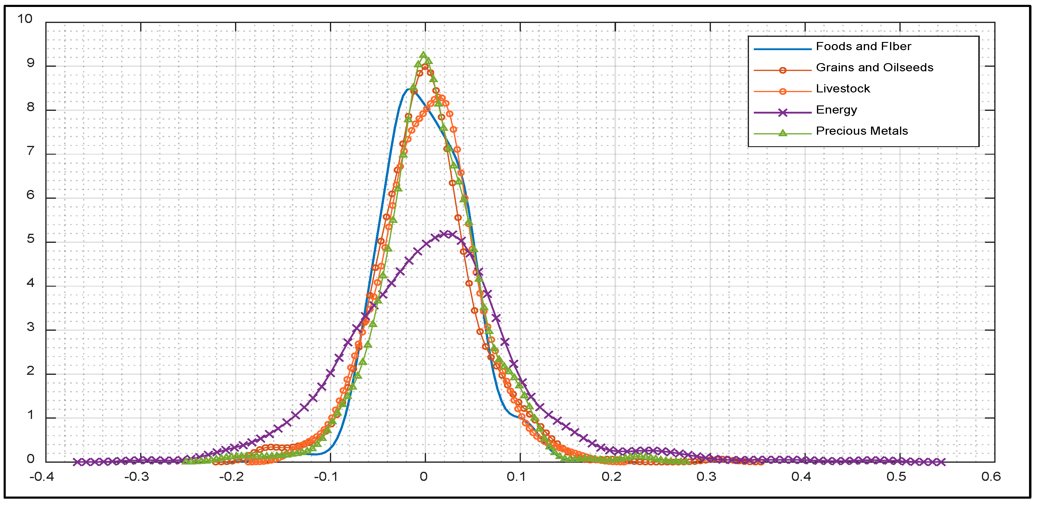
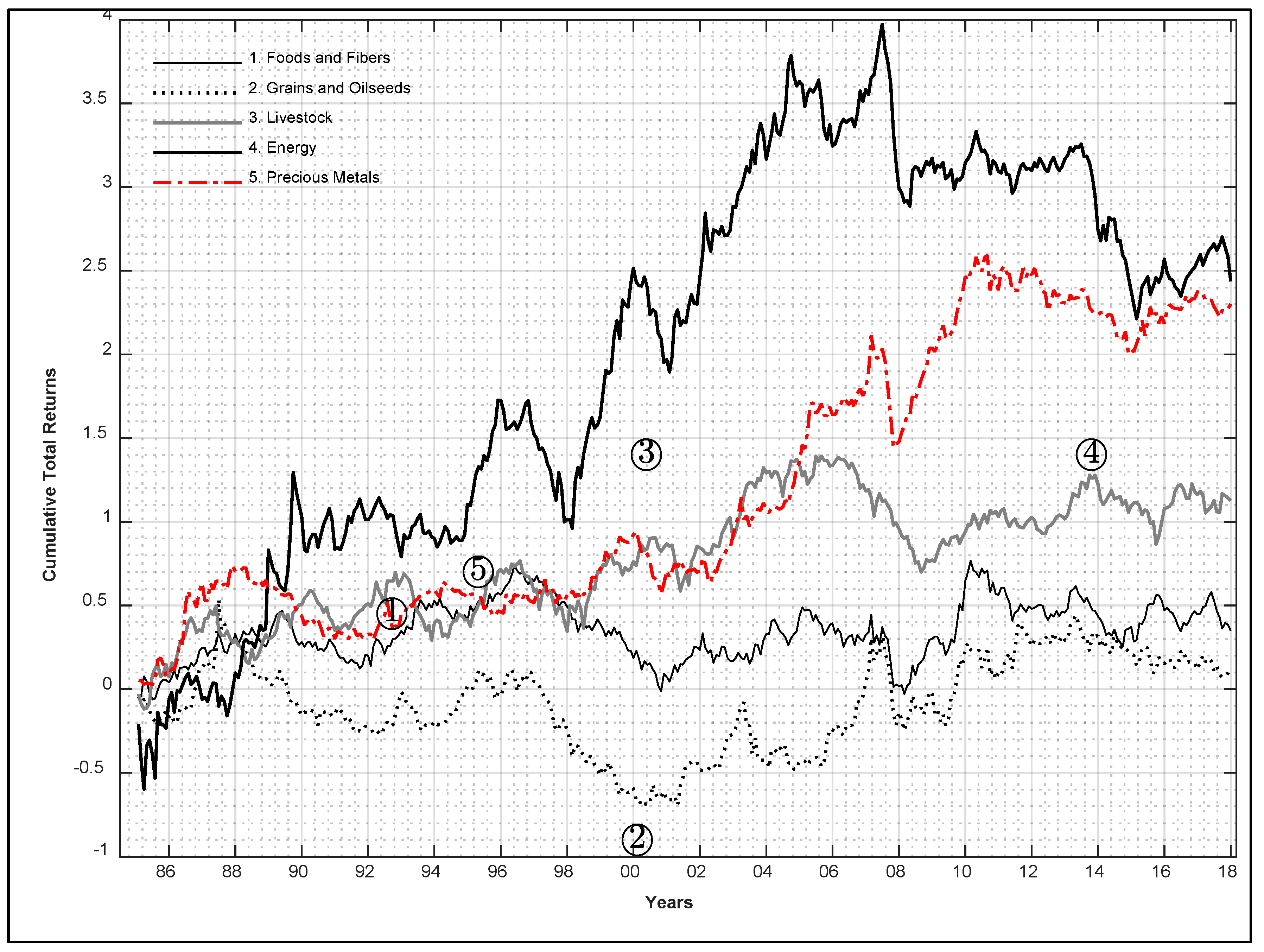
3.1. Sectoral Risk and Returns Analysis

The underlying commodities we use in this study are diverse. Such diversity tends to manifest itself in smaller return correlations between constituents of different sectors rather than members categorized within the same sector (Adhikari and Putnam 2020). This heterogeneity can be viewed through the lens of distributional returns. Figure 1 plots the return distributions of the five commodity sectors. The energy sector exhibits a noticeable positive moderate skewness. The three other commodity sectors show little, if any, skewness. The foods and fibers, as well as livestock sectors, demonstrate slim, light tails (platykurtic) while the other return distributions more or less follow a standard normal distribution. Finally, the varying “peakedness” of the sector distributions highlights the potential usefulness of robust estimation in developing optimal portfolio allocations because of the marked dissimilarities.
Figure 2 provides additional insights into the return behavior of the commodity sectors. In terms of cumulative total returns, the energy and precious metal sectors are the run-away winners. In contrast, the grains and oilseeds sectors are the worst performers during the sample period. Most of the commodity sectors show favorable performance in the early-to-mid 2000s, followed by a sharp downturn coinciding with the 2008 global financial crisis. Yet, it is apparent that the sectors do not comove together strongly. An equally weighted investment in the five commodity sectors seemingly yields obvious diversification benefits. However, the question we seek to answer is how the robust optimization-based portfolios perform compared to such a naïve buy-and-hold benchmark composed of the same constituents.
Table 3 summarizes the key performance metrics of the commodity sectors used in our analysis. As shown in the table, the energy sector yields the highest average (cumulative) return of 7.64% (243.72%) among the five commodity sectors. The precious metals sector narrowly follows the energy sector with an average (cumulative) return of 7.20% (230.11%), followed by the livestock sector, which lags further with an average (cumulative) return of 3.47% (112.74%). Interestingly, the foods and fibers and the grains and oilseeds sectors yield significantly lower average (cumulative) returns of 1.07% (35.01%) and 0.20% (6.58%), respectively. The table also indicates that the energy sector has the highest volatility with an annualized standard deviation of 31.38%; this is roughly 1.5 to 2 times that of the other commodity sectors. The precious metals, energy, and livestock sectors offer the best risk-adjusted returns (i.e., Sharpe, Treynor, and Sortino ratios), respectively.
The results presented in Table 3 show interesting variation in terms of both returns and risk across the commodity groups. While returns and volatility are useful metrics for understanding asset behavior, an essential component for evaluating performance is potential severe loss scenarios. Since extreme fluctuations can be detrimental to returns, we look at both value-at-risk (VaR) and conditional value-at-risk. Based on all statistical measures, the energy sector is the most susceptible and prone to significant losses, followed by precious metals and the grains and oilseeds sectors. Overall, there is tremendous variation in the performance profiles among the five commodity sectors. Therefore, the groups serve our objective of a diverse set of investments to use in the robust optimization portfolio formation process.

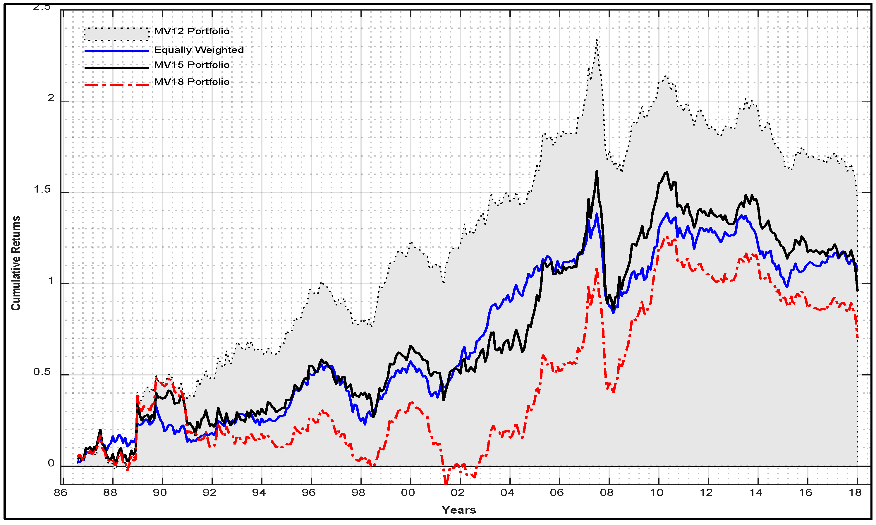
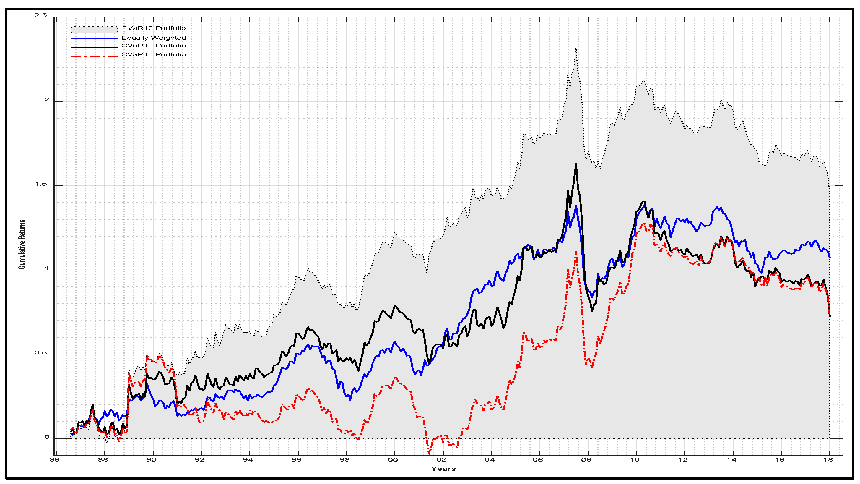
3.2. Portfolio Risk and Returns

Figure 3 shows the cumulative returns of the naïve buy-and-hold equally weighted commodity futures portfolio relative to the MV robust optimization-based portfolios for the sample period from January 1986 to December 2018. The figure illustrates a “horse race” of sorts between the MV12, MV15, and MV18 portfolios against the benchmark. The MV12 pointedly outperforms the equally weighted benchmark, over virtually the entire sample period. The MV15 portfolio both outperforms and underperforms the benchmark portfolio over time, ultimately underachieving relative to the benchmark when the sample period ends. The MV18 portfolio underperforms the passive benchmark portfolio over the entire sample.
Similarly, Figure 4 shows a horse race for the CVaR optimization-based portfolios relative to the long-only naïve benchmark. The findings in relation to the lookback periods are quite similar to the mean-variance portfolios in Figure 3. The CVaR12 markedly outperforms the equally weighted benchmark. The CVaR15 portfolio over and underperforms the benchmark at various points over the sample period, ultimately falling short of the benchmark portfolio by the end of 2018. The CVaR18 portfolio consistently performs the worst of all robust optimization-based portfolios. However, unlike the MV18 portfolio, the CVaR18 portfolio performance tends to hug much closer to the 15-month look back portfolio (i.e., CVaR15) post-2008. Overall, it is apparent that the robust estimation procedure utilizing a 12-month lookback period performs far superior to the other portfolios conditioned on longer lookback periods.
Table 4 summarizes the performance metrics for the benchmark portfolio and all the robust optimization-based portfolios. Following standard practices in the commodity literature (Rad et al. 2020; Bakshi et al. 2017; Erb and Harvey 2006; Miffre and Rallis 2007; Szymanowska et al. 2014), we compare the performance of the sophisticated robust optimization-based portfolios to the equally weighted buy-and-hold benchmark. The average (cumulative) returns for the best-performing MV12 and CVaR12 portfolios are the 4.72% (145.42%) and 4.69% (144.58%); in contrast, the returns for the benchmark portfolio (EW) are 3.46% (107.21%). The annualized standard deviations of MV12 and CVaR12 are 15.59% and 15.55%, respectively. The benchmark portfolio, on the other hand, only has a standard deviation of 11.41%. The standard deviations of the 15- and 18-month lookback portfolios are all higher than their comparable 12-month counterpart, even though these portfolios have lower returns.
Given the disparity in return and risk measures between the MV12 and CVaR12 portfolios and the equally weighted benchmark portfolio, it is natural to compare risk-adjusted returns to see if, in fact, the outperformance of the 12-month lookback portfolios is simply due to increased portfolio risk. The risk-adjusted measures, namely the Sharpe, Treynor, and Sortino ratios, elucidate the superiority of the MV12 and CVaR12 portfolios. In all cases, the risk-adjusted measures are superior to that of the benchmark portfolio. The same is not true of the 15- and 18-month look back portfolios. Hence, the outperformance of the MV12 and CVaR12 portfolios can be attributed to the optimal allocations through robust estimation. These results are consistent with the findings of Zhang et al. (2017) who find that a robust futures strategy outperforms a corresponding non-robust strategy in out-of-sample tests in the face of ambiguity aversion. We conclude that the performance of an equally weighted benchmark portfolio is suboptimal compared to the MV12 and CVaR12 robust optimization portfolios. Our findings highlight the benefits of applying sophisticated, robust optimization while forming a portfolio consisting of commodity futures. This view has also recently found support within the research of Rad et al. (2020). They document the benefits of applying a sophisticated weighting scheme to enhance the performance of long-short commodity portfolios.

3.3. Optimal Performance by Holding Period

Given that the 12-month lookback and 1-month holding period provides superior return results against the benchmark portfolio for both the MV and CVaR optimization methodologies, we further investigate the properties of these portfolios by looking at various holding periods to see if the performance metrics can be further enhanced. Table 5 presents the results for the MV12 portfolio by holding period, where “HP” refers to holding period, and the succeeding integer refers to the number of months the weights are maintained before the portfolio is rebalanced. The statistics in the second column (HP1) correspond to the results found in the third column of Table 4 (MV12)—this is obvious since the initial portfolio analysis was conducted using only 1-month holding periods. For instance, the average (cumulative) return for the three-month holding period portfolio (HP3) is 3.27% (101.40%). We consistently find that as the holding period is extended, there is a decline in the portfolio’s return—that is, there is an inverse relationship between holding period and portfolio return performance for the arithmetic, geometric, and cumulative returns. Risk-adjusted measures have an inverse relationship as well, despite no obvious correlation emerging between the holding period and portfolio standard deviation. Overall, we find a reasonable increase in the value-at-risk measures as the holding period increases. The rise in risk is not linear, but it is clear that longer holding periods equate to additional value-at-risk while achieving lower average returns.
Table 6 shows the metrics for the CVaR12 portfolio by holding period. The statistics for the CVaR12 portfolio across the five different holding periods mirrors that of the MV12 portfolio. For instance, an inverse relationship exists between the holding period and returns, as well as the holding period and risk-adjusted measures. Value-at-risk also rises in a non-linear fashion with the holding period. Taken together, Table 5 and Table 6 clearly demonstrate that a 1-month holding period (i.e., HP1) generates superior return performance at a lower risk compared to the other holding periods, regardless of optimization methodology chosen.

4. Concluding Remarks

This paper studies commodity futures returns over the 33-year period ranging from January 1986 to December 2018. In order to address data uncertainty faced by investors, we utilize robust estimation to form commodity portfolios using both the conventional MV and CVaR framework. First, we create robust optimization-based portfolios by conditioning on prior return data using 12-, 15-, or 18-month lookback periods to generate the covariance matrix. Next, we simulate the return-risk outcomes for each lookback window using the respective sample mean vector and covariance matrix to create the optimal portfolio weights for each commodity sector. Finally, the portfolios are held for one month and are then recalibrated for the next one month holding period on a rolling basis. In total, we analyze the performance metrics of three MV robust optimization-based portfolios over three lookback periods and three CVaR robust optimization-based portfolios over the same three lookback periods.
The performance of the robust portfolios is compared against a naïve equally weighted buy-and-hold benchmark portfolio of commodity futures. The results indicate that portfolios constructed using robust optimization with a 12-month lookback (MV12 and CVaR12) outperform both the benchmark portfolio as well as the other robust optimization-based portfolios. These findings suggest that the utility of historical returns beyond 12 months sharply deteriorates when used as input in forming robust portfolio weights. Our findings are consistent with Kim et al. (2017) that robust optimization-based portfolios can offer returns well beyond what a passive benchmark can offer. However, our findings are qualified, as only a lookback period of 12 months produces superior risk-adjusted returns. A more in-depth analysis of the holding period for the MV12 and CVarR12 portfolios shows that the 1-month holding period is optimal. Overall, our findings suggest that the naïve equally weighting scheme traditionally employed in commodity portfolio constructions can be enhanced by using the sophisticated, robust optimization technique.
The key contributions of this paper are to address data uncertainty faced by investors in the commodity futures markets, evaluate the performance of robust-optimized portfolios against a buy-and-hold equally weighted portfolio, and examine the most informative lookback and holding periods in the commodity portfolio formation process. Our findings suggest that the naïve equally weighted scheme traditionally employed in the portfolio formation process can be improved by the use of a more sophisticated robust optimization technique. A practical implementation of robust optimization in the financial markets may provide valuable benefits to investors. The methodology can efficiently handle a class of interior-point optimizers that are capable of managing second-order constraints and can produce better weights than the classical mean-variance approach under uncertainty. Nonetheless, while risk-adjusted returns outperform a naïve benchmark, an implementation of this approach will have more value-at-risk for investors.

Author Contributions

All three authors spent equal amount of time and effort in completing this paper. All authors have read and agreed to the published version of the manuscript.

Funding

This research received no external funding.

Conflicts of Interest

The authors declare no conflict of interest.

References

  1. Adhikari, Ramesh, and Kyle J. Putnam. 2020. Comovement in the Commodity Futures Markets: An Analysis of the Energy, Grains, and Livestock Sectors. Journal of Commodity Markets 18: 100090. [Google Scholar] [CrossRef]
  2. Asness, Clifford S., Tobias J. Moskowitz, and Lasse Heje Pedersen. 2013. Value and Momentum Everywhere. Journal of Finance 68: 929–85. [Google Scholar] [CrossRef] [Green Version]
  3. Bakshi, Gurdip, Xiaohui Gao, and Alberto G. Rossi. 2017. Understanding the Sources of Risk Underlying the Cross Section of Commodity Returns. Management Science 65: 619–41. [Google Scholar] [CrossRef] [Green Version]
  4. Best, Michael J., and Robert R. Grauer. 1991. On the Sensitivity of Mean-Variance-Efficient Portfolios to Changes in Asset Means: Some Analytical and Computational Results. Review of Financial Studies 4: 315–432. [Google Scholar] [CrossRef] [Green Version]
  5. Bhardwaj, Geetesh, Gary Gorton, and K. Geert Rouwenhorst. 2015. Facts and Fantasies about Commodity Futures Ten Years Later. NBER Working Paper Series; New York: National Bureau of Economic Research, Inc., pp. 1–29. [Google Scholar]
  6. Bi, Junna, Hanqing Jin, and Qingbin Meng. 2018. Behavioral Mean-Variance Portfolio Selection. European Journal of Operational Research 271: 644–63. [Google Scholar] [CrossRef]
  7. Black, Fischer, and Robert Litterman. 1992. Global Portfolio Optimization. Financial Analysts Journal 48: 28–43. [Google Scholar] [CrossRef]
  8. Calafiore, Giuseppe C. 2007. Ambiguous Risk Measures and Optimal Robust Portfolios. SIAM Journal on Optimization 18: 853–77. [Google Scholar] [CrossRef]
  9. Ceria, Sebastián, and Robert A. Stubbs. 2006. Incorporating Estimation Errors into Portfolio Selection: Robust Portfolio Construction. Journal of Asset Management 7: 109–27. [Google Scholar] [CrossRef]
  10. DeMiguel, Victor, Lorenzo Garlappi, and Raman Uppal. 2009. Optimal versus Naive Diversification: How Inefficient Is the 1/N Portfolio Strategy? Review of Financial Studies 22: 1915–53. [Google Scholar] [CrossRef] [Green Version]
  11. Elliott, Robert J., and Tak Kuen Siu. 2010. On Risk Minimizing Portfolios under a Markovian Regime-Switching Black-Scholes Economy. Annals of Operations Research 176: 271–91. [Google Scholar] [CrossRef]
  12. Erb, Claude B., and Campbell R. Harvey. 2006. The Strategic and Tactical Value of Commodity Futures. Financial Analysts Journal 62: 125–78. [Google Scholar] [CrossRef]
  13. Fan, Jianqing, Yingying Fan, and Jinchi Lv. 2008. High Dimensional Covariance Matrix Estimation Using a Factor Model. Journal of Econometrics 147: 186–97. [Google Scholar] [CrossRef] [Green Version]
  14. Goldfarb, Donald, and Garud Iyengar. 2003. Robust Portfolio Selection Problems. Mathematics of Operations Research 28: 1–38. [Google Scholar] [CrossRef]
  15. Gorton, Gary, and K. Geert Rouwenhorst. 2006. Facts and Fantasies about Commodity Futures. Financial Analysts Journal 62: 47–68. [Google Scholar] [CrossRef] [Green Version]
  16. Grauer, Robert R., and Frederick C. Shen. 2000. Do Constraints Improve Portfolio Performance? Journal of Banking and Finance 24: 1253–74. [Google Scholar] [CrossRef]
  17. Green, Richard C., and Burton Hollifield. 1992. When Will Mean-Variance Efficient Portfolios Be Well Diversified? The Journal of Finance 47: 1785–809. [Google Scholar] [CrossRef]
  18. Huang, Xiaoxia, and Tingting Yang. 2020. How Does Background Risk Affect Portfolio Choice: An Analysis Based on Uncertain Mean-Variance Model with Background Risk. Journal of Banking and Finance 111: 105726. [Google Scholar] [CrossRef]
  19. Huo, Lijuan, Tae-Hwan Kim, and Yunmi Kim. 2012. Robust Estimation of Covariance and Its Application to Portfolio Optimization. Finance Research Letters 9: 121–34. [Google Scholar] [CrossRef]
  20. Jensen, Michael C. 1968. Problems in the Selection of Security Portfolios—The Performance of Mutual Funds in the Period 1945–1964. Journal of Finance 23: 389–416. [Google Scholar] [CrossRef]
  21. Jorion, Philippe. 1986. Bayes-Stein Estimation for Portfolio Analysis. The Journal of Financial and Quantitative Analysis 21: 279–92. [Google Scholar] [CrossRef]
  22. Kim, Tae-Hwan, and Halbert White. 2004. On More Robust Estimation of Skewness and Kurtosis. Finance Research Letters 1: 56–73. [Google Scholar] [CrossRef]
  23. Kim, Jang Ho, Woo Chang Kim, and Frank J. Fabozzi. 2013. Composition of Robust Equity Portfolios. Finance Research Letters 10: 72–81. [Google Scholar] [CrossRef]
  24. Kim, Woo Chang, Jang Ho Kim, and Frank J. Fabozzi. 2016. Robust Equity Portfolio Management + Website: Formulations, Implementations and Properties Using MATLAB, 1st ed. Hoboken: John Wiley & Sons, Inc. [Google Scholar]
  25. Kim, Jang Ho, Woo Chang Kim, Do-Gyun Kwon, and Frank J. Fabozzi. 2017. Robust Equity Portfolio Performance. Annals of Operations Research 266: 293–312. [Google Scholar] [CrossRef]
  26. Lim, Andrew E. B., Jeyaveerasingam George Shanthikumar, and Gah-Yi Vahn. 2011. Conditional Value-at-Risk in Portfolio Optimization: Coherent but Fragile. Operations Research Letters 39: 163–71. [Google Scholar] [CrossRef]
  27. Lwin, Khin T., Rong Qu, and Bart L. MacCarthy. 2017. Mean-VaR Portfolio Optimization: A Nonparametric Approach. European Journal of Operational Research 260: 751–66. [Google Scholar] [CrossRef] [Green Version]
  28. Markowitz, Harry. 1952. Portfolio Selection. The Journal of Finance 7: 77–91. [Google Scholar]
  29. Michaud, Richard O. 1998. Efficient Asset Management: A Practical Guide to Stock Portfolio Optimization and Asset Allocation. Boston: Oxford University Press. [Google Scholar]
  30. Michaud, Richard O., and Robert Michaud. 2008. Estimation Error and Portfolio Optimization: A Resampling Solution. Journal of Investment Management 6: 8–28. [Google Scholar] [CrossRef] [Green Version]
  31. Miffre, Joëlle, and Georgios Rallis. 2007. Momentum Strategies in Commodity Futures Markets. Journal of Banking and Finance 31: 1863–86. [Google Scholar] [CrossRef]
  32. Moskowitz, Tobias J., Yao Hua Ooi, and Lasse Heje Pedersen. 2012. Time Series Momentum. Journal of Financial Economics 104: 228–50. [Google Scholar] [CrossRef] [Green Version]
  33. Natarajan, Karthik, Dessislava Pachamanova, and Melvyn Sim. 2009. Constructing Risk Measures from Uncertainty Sets. Operations Research 57: 1129–41. [Google Scholar] [CrossRef] [Green Version]
  34. Post, Thierry, Selçuk Karabatı, and Stelios Arvanitis. 2019. Robust Optimization of Forecast Combinations. International Journal of Forecasting 35: 910–26. [Google Scholar] [CrossRef]
  35. Rad, Hossein, Rand Kwong Yew Low, Joëlle Miffre, and Robert Faff. 2020. Does Sophistication of the Weighting Scheme Enhance the Performance of Long-Short Commodity Portfolios? Journal of Empirical Finance 58: 164–80. [Google Scholar] [CrossRef]
  36. Rockafellar, Ralph Tyrrell, and Stanislav Uryasev. 2000. Optimization of Conditional Value-at-Risk. The Journal of Risk 2: 21–41. [Google Scholar] [CrossRef] [Green Version]
  37. Scherer, Bernd. 2007. Can Robust Portfolio Optimisation Help to Build Better Portfolios? Journal of Asset Management 7: 374–87. [Google Scholar] [CrossRef] [Green Version]
  38. Sharpe, William F. 1964. Capital Asset Prices: A Theory of Market Equilibrium Under Conditions of Risk. The Journal of Finance 19: 425–42. [Google Scholar]
  39. Shen, Ruijun, and Shuzhong Zhang. 2008. Robust Portfolio Selection Based on a Multi-Stage Scenario Tree. European Journal of Operational Research 191: 864–87. [Google Scholar] [CrossRef]
  40. Szymanowska, Marta, Frans de Roon, Theo Nijman, and Rob van den Goorbergh. 2014. An Anatomy of Commodity Futures Risk Premia. Journal of Finance 69: 453–82. [Google Scholar] [CrossRef]
  41. Tütüncü, Reha H., and Mark Koenig. 2004. Robust Asset Allocation. Annals of Operations Research 132: 157–87. [Google Scholar] [CrossRef] [Green Version]
  42. Zakamulin, Valeriy. 2017. Superiority of Optimized Portfolios to Naive Diversification: Fact or Fiction? Finance Research Letters 22: 122–28. [Google Scholar] [CrossRef]
  43. Zhang, Jinqing, Zeyu Jin, and Yunbi An. 2017. Dynamic Portfolio Optimization with Ambiguity Aversion. Journal of Banking and Finance 79: 95–109. [Google Scholar] [CrossRef]
  44. Zhu, Shushang, and Masao Fukushima. 2009. Worst-Case Conditional Value-at-Risk with Application to Robust Portfolio Management. Operations Research 57: 1155–68. [Google Scholar] [CrossRef]
1
In practice, there are many different definitions of robustness based on various mathematical formulations. See Kim et al. (2016) for an overview of several optimization methodologies.
2
It is worth noting that there is an elliptical constraint on the standard deviation of returns in Kim et al. (2017) that is not assumed in our robust estimation process which may impact on the discrepancy in findings.
3
Returns are always calculated on the same contract and we do not include the return on collateral associated with the futures contract in the calculation.
4
Asness et al. (2013) and Moskowitz et al. (2012) create a monthly series with the same procedure; specifically, to convert the daily returns to monthly returns the following formula is applied: R Month = ( i day ( r i 100 + 1 ) 1 ) .
5
In fact, when the past 24 months of return data are used in the robust portfolio optimization process, both the MV and CVaR portfolios further underperform the naïve buy-and-hold benchmark.
Figure 1. Empirical Distributions of Monthly Commodity Futures’ Sector Returns. Notes: This figure shows the distribution of monthly returns for the five commodity sectors over the sample period from January 1986 to December 2018. “Foods” represents the foods and fibers sector, “Grains” represents the grains and oilseeds sector, and “Metals” represents the precious metals sector.
Ijfs 08 00054 g001
Figure 2. Cumulative Monthly Returns by Commodity Sector. Notes: This figure shows the cumulative monthly returns of the five commodity sectors used in this study for January 1986 to December 2018.
Ijfs 08 00054 g002
Figure 3. Performance of Equally Weighted and MV Optimization-based Commodity Portfolios. Notes: This figure shows the cumulative return for the naïve buy-and-hold benchmark portfolio relative to the mean-variance robust optimization-based portfolios over the sample period from January 1986 to December 2018. Equally weighted represents the naïve buy-and-hold benchmark portfolio. MV12, MV15, and MV18 represent the robust optimization-based mean-variance portfolios that use a 12-month, 15-month, and 18-month lookback period of returns, respectively, with a one-month portfolio holding period.
Ijfs 08 00054 g003
Figure 4. Performance of Equally Weighted and CVaR Optimization-based Commodity Portfolios. Notes: This figure shows the cumulative return for the naïve buy-and-hold benchmark portfolio relative to the robust optimization-based portfolios over the sample period from January 1986 to December 2018. Equally weighted represents the naïve buy-and-hold benchmark portfolio. CVaR12, CVaR15, and CVar18 represent the robust optimization-based conditional value-at-risk portfolios that use a 12-month, 15-month, and 18-month lookback period of returns, respectively, with a one-month portfolio holding period.
Ijfs 08 00054 g004
Table 1. Commodity Futures by Sector.
SectorCommodities
Foods and FibersCocoa, Coffee, Orange Juice, Sugar #11, Cotton, Lumber
Grains and OilseedsCorn #2, Oats, Rough Rice #2, Soybeans, Soybean Meal, Soybean Oil, Wheat, Barley, Canola
LivestockFeeder Cattle, Live Cattle, Lean Hogs, Pork Bellies
EnergyCrude Oil, Heating Oil #2, Unleaded Gas, Natural Gas, Propane
Precious MetalsCopper, Gold, Palladium, Platinum, Silver
Notes: This table shows the commodity futures represented in each commodity sector. All commodity futures prices are extracted from the Commodity Research Bureau (CRB).
Table 2. Performance Metrics.
Performance MetricDescription
Arithmetic meanReported as the average monthly return expressed as an annualized percentage.
Standard deviationReported as the average monthly standard deviation expressed as an annualized percentage.
Geometric meanReported as the average monthly return expressed as an annualized percentage.
Cumulative returnReported as the portfolio return over the full sample period.
Sample skewnessReported as a monthly average.
Sample excess kurtosisReported as a monthly average.
Sharpe ratioReported as the average excess monthly return divided by the monthly standard deviation, where the risk-free rate is obtained from Ken French’s website.
Tracking errorReported as the monthly average standard deviation of the difference between a commodity portfolio returns and the value-weighted market index of returns from the Center for Research in Security Prices (CRSP). The CRSP market index return is obtained from Ken French’s website.
Information ratioReported as the excess monthly return of a portfolio in excess of the CRSP value-weighted market index of returns divided by the tracking error.
CAPM alphaReported as the average monthly alpha computed following Jensen (1968) expressed as an annualized percentage, where the market factor is obtained from Ken French’s website.
CAPM betaReported as the average monthly beta computed following Sharpe (1964), where the market factor is obtained from Ken French’s website.
Treynor ratioReported as the average excess monthly return divided by the monthly portfolio beta, where the risk-free rate is obtained from Ken French’s website.
Sortino ratioReported as the average excess monthly return divided by the monthly standard deviation of negative asset returns, where the risk-free rate is obtained from Ken French’s website.
Historical 95% VaRReported as the average expected 1-month loss with 95% certainty, based on historical returns.
Normal 95% VaRReported as the average expected 1-month loss with 95% certainty, under normality.
Historical 95% CVaRReported as the average expected 1-month loss beyond the VaR with 95% certainty, based on normality.
Normal 95% CVaRReported as the average expected 1-month loss beyond the VaR with 95% certainty, based on historical returns.
M-squareReported as the average monthly return of a portfolio plus the product of the average monthly Sharpe ratio of the equally weighted benchmark and the average deviation of the standard deviation of the portfolio under consideration from the benchmark portfolio.
Notes: This table shows the description of the performance metrics that are calculated for all commodity portfolios. The Ken French data library for the broad market and risk-free data can be found at https://mba.tuck.dartmouth.edu/pages/faculty/ken.french/data_library.html.
Table 3. Performance by Commodity Sector.
StatisticsFoodsGrainsLivestockEnergyMetals
Arithmetic Mean (%)1.06620.19963.47037.64067.2003
Standard Deviation (%)15.700819.110817.049231.384518.2431
Geometric Mean (%)−0.1667−1.59851.98632.64065.4434
Cumulative Returns (%)35.01316.5806112.7373243.7192230.1109
Sample Skewness0.13280.38620.06070.69090.0068
Sample Excess Kurtosis0.93563.10460.45673.09752.3497
Sharpe Ratio (%)−0.0384−0.04460.00450.03900.0605
Tracking Error (%)0.05600.06480.06460.09710.0607
Information Ratio (%)−0.1466−0.1377−0.0966−0.0302−0.0539
CAPM Alpha (%)0.22010.20080.04420.18180.2621
CAPM Beta0.00400.00080.06450.03390.0222
Treynor Ratio (%)−0.1460−0.1362−0.0964−0.0301−0.0539
Sortino Ratio (%)−0.0539−0.06300.00640.06050.0900
Historical 95% VaR6.52608.67367.905213.51378.0517
Normal 95% VaR7.36689.05777.810814.28688.0812
Historical 95% CVaR9.024112.323110.181617.822011.4665
Normal 95% CVaR9.260711.36309.867318.072610.2818
M-Square (%)−0.0081−0.0084−0.0063−0.0048−0.0038
Notes: This table presents the performance metrics for each commodity sector over the sample period from January 1986 to December 2018. The sector returns are constructed by averaging the monthly futures returns assigned to each group. “Foods” represents the foods and fibers sector, “Grains” represents the grains and oilseeds sector, and “Metals” represents the precious metals sector.
Table 4. Performance Metrics by Commodity Portfolio.
StatisticsEWMV12MV15MV18CVaR12CVAR15CVaR18
Arithmetic Mean (%)3.45714.71563.08532.24824.68762.30932.3355
Standard Deviation (%)11.414315.586315.884016.066715.551315.629416.0739
Geometric Mean (%)2.78003.47141.77920.96293.44931.05371.0478
Cumulative Returns (%)107.2094145.424995.839070.1003144.577971.983272.7921
Sample Skewness−0.58600.6603−0.25340.86130.6664−0.25700.8595
Sample Excess Kurtosis3.112912.07466.708810.625412.19786.119210.7345
Sharpe Ratio (%)0.00950.02940.0003−0.01440.0290−0.0137−0.0129
Tracking Error (%)0.04770.05550.05610.05730.05550.05600.0573
Information Ratio (%)−0.1181−0.0834−0.1057−0.1155−0.0838−0.1172−0.1142
CAPM Alpha (%)0.18520.22180.22310.20140.22050.20840.2014
CAPM Beta0.01530.01730.01140.00920.01730.00910.0096
Treynor Ratio (%)−0.1192−0.0823−0.1059−0.1129−0.0827−0.1174−0.1117
Sortino Ratio (%)0.01290.04440.0004−0.02130.0437−0.0189−0.0190
Historical 95% VaR5.09985.85836.71286.43425.89086.67516.3910
Normal 95% VaR5.13627.01617.28867.44357.00177.23097.4398
Historical 95% CVaR7.73019.222210.679210.28529.218710.761110.2213
Normal 95% CVaR6.51308.89629.20469.38158.87769.11629.3787
M-Square (%)−0.0055−0.0047−0.0059−0.0066−0.0047−0.0065−0.0065
Notes: This table shows the performance metrics for the commodity portfolios over the sample period from January 1986 to December 2018. EW represents the naïve buy-and-hold benchmark. MV12, MV15, and MV18 represent the robust optimization-based mean-variance portfolios that use a 12-month, 15-month, and 18-month lookback period of returns, respectively. Similarly, CVaR12, CVaR15, and CVar18 represent the robust optimization-based conditional value-at-risk portfolios that use a 12-month, 15-month, and 18-month lookback period of returns, respectively.
Table 5. Performance Metrics by Holding Period for MV Optimization Portfolio using a 12-Month Lookback Period.
StatisticsHP1HP3HP6HP9HP12
Arithmetic Mean (%)4.71563.26703.21492.97772.8339
Standard Deviation (%)15.586316.212916.102215.940816.4617
Geometric Mean (%)3.47141.93521.90331.68931.4789
Cumulative Returns (%)145.4249101.399799.806092.541688.1293
Sample Skewness0.66030.57840.59690.41590.7399
Sample Excess Kurtosis12.074610.446210.02137.66996.2305
Sharpe Ratio (%)0.02940.00340.0025−0.0016−0.0040
Tracking Error (%)0.05550.05660.05610.05820.0589
Information Ratio (%)−0.0834−0.1023−0.1040−0.1035−0.1042
CAPM Alpha (%)0.22180.23330.24040.16440.1804
CAPM Beta0.01730.01150.01100.01490.0129
Treynor Ratio (%)−0.0823−0.1008−0.1025−0.1024−0.1026
Sortino Ratio (%)0.04440.00500.0037−0.0024−0.0061
Historical 95% VaR5.85836.55226.90926.55166.7393
Normal 95% VaR7.01617.43017.38177.32437.5833
Historical 95% CVaR9.22229.957810.22249.95309.9973
Normal 95% CVaR8.89629.38589.32419.24729.5690
M-Square (%)−0.0047−0.0058−0.0058−0.0060−0.0061
Notes: This table shows the performance metrics for the mean-variance optimization-based commodity portfolios utilizing a 12-month lookback by holding period, over the sample period January 1986 to December 2018. HP1, HP3, HP6, HP9, and HP12 represent the 1-, 3-, 6-, 9-, and 12-month portfolio holding periods, respectively.
Table 6. Performance Metrics by Holding Period for CVaR Optimization Portfolio using 12-Month Lookback Period.
StatisticsHP1HP3HP6HP9HP12
Arithmetic Mean (%)4.68783.14523.13132.97322.8119
Standard Deviation (%)15.551316.161516.048615.929916.3438
Geometric Mean (%)3.44951.82291.82901.68761.4750
Cumulative Returns (%)144.583697.674497.247392.403187.4524
Sample Skewness0.66650.57380.59110.44860.6995
Sample Excess Kurtosis12.197810.552810.10237.86845.8570
Sharpe Ratio (%)0.02900.00130.0011−0.0017−0.0044
Tracking Error (%)0.05550.05640.05590.05820.0586
Information Ratio (%)−0.0838−0.1044−0.1055−0.1036−0.1051
CAPM Alpha (%)0.22050.23450.24170.16430.1807
CAPM Beta0.01730.01100.01060.01490.0128
Treynor Ratio (%)−0.0827−0.1028−0.1039−0.1024−0.1035
Sortino Ratio (%)0.04370.00190.0016−0.0025−0.0067
Historical 95% VaR5.89086.56746.92116.56306.7529
Normal 95% VaR7.00177.41567.36317.31957.5291
Historical 95% CVaR9.21869.968810.22559.93689.9135
Normal 95% CVaR8.87769.36519.29909.24119.5006
M–Square (%)−0.0047−0.0059−0.0059−0.0060−0.0061
Notes: This table shows the performance metrics for the conditional value-at-risk optimization-based commodity portfolios utilizing a 12-month lookback by holding period, over the sample period January 1986 to December 2018. HP1, HP3, HP6, HP9, and HP12 represent the 1-, 3-, 6-, 9-, and 12-month portfolio holding periods, respectively.

