Abstract
The Turn of the month effect is one of the better-known calendar anomalies. If a stock market is affected by the Turn of the month effect, it records significantly higher returns during a relatively short time period around the end of the old month and the beginning of the new one, than during the remainder of the month. This paper investigates the presence of the Turn of the month effect in the stock markets of 11 Central and Eastern European (CEE) countries. We focused not only on the anomaly in returns, but also on the anomaly in price volatility. The results show that, during a 20-year period (1999–2018), a statistically significant Turn of the month effect was present in the stock markets of seven out of 11 investigated countries. However, the anomaly affected only the stock market returns, not price volatility.
Keywords:
turn of the month effect; calendar anomaly; stock market; CEE; JEL Classification:
G01; G14; G15
1. Introduction
The Central and Eastern European (CEE) stock markets, with the exception of Turkey, are relatively young. They were established during the 1990s, after the collapse of the centrally planned economies and transition to market economy. Although they keep on evolving, they still face various issues. Especially, their liquidity tends to be lower in comparison to the developed stock markets of Western Europe and North America. In recent years, numerous authors paid attention to various issues that were related to the CEE stock markets as a group, or to some individual countries.
In this paper, we aim to extend the current state of knowledge regarding the CEE stock markets. More specifically, we focus on the investigation of presence of the Turn of the month effect on the stock markets of 11 CEE region countries.
The Turn of the month effect is one of the calendar anomalies that have been identified over the recent decades. Multiple studies confirm that various calendar anomalies can be found in stock (but also bond and commodity) markets around the world (Lakonishok and Smidt 1988; Milonas 1991; Giovanis 2009; Borowski 2015). According to Bouman and Jacobsen (2002), one of them, the Halloween effect, can be tracked back to the late 17th century. Although the strength of the calendar anomalies changes over time, several studies confirm that, in the long-term, they can be exploited to generate abnormal returns (Kunkel and Compton 1998; Andrade et al. 2013; Dichtl and Drobetz 2015).
The main feature of the Turn of the month effect is an uneven distribution of stock market returns during the month. More specifically, if the Turn of the month effect is present in a particular stock market, the majority of returns are concentrated in the turn of the month period, which can be defined as several days at the end of the old month and the beginning of the new one. Some studies even conclude that almost all of the positive stock market returns are concentrated in a short period of several days around the turn of the month (Lakonishok and Smidt 1988; McConnell and Xu 2008).
In this paper, we investigate the presence of the Turn of the month effect on stock markets of 11 CEE region countries, during the time period that spans from January 1999 to December 2018. However, we focus not only on the presence of the Turn of the month effect in the stock market returns, but also on its presence in stock market volatilities. As the vast majority of studies focuses only on returns, we believe that the analysis of the relation of the Turn of the month effect and the stock market volatilities might be an important addition to the current state of knowledge. Moreover, the presence of the Turn of the month effect in the CEE region may confirm the lack of efficiency of these markets (as defined by Fama 1965), as the calendar anomalies can often be used in the investment process to generate abnormal returns.
2. Literature Review
The Turn of the month effect is one of the better known calendar anomalies that impact the stock markets, such as the Day of the week effect, the Halloween effect, the January effect, the Holiday effect, etc.
The Day of the Week effect was studied by Aggarwal and Schatzberg (1997), Philpot and Peterson (2011) or Brusa and Liu (2004). This calendar anomaly is based on the tendency of the stock market to record significantly better or worse returns during a particular day of the week. The returns usually tend to be higher on Fridays and lower on Mondays.
The Halloween effect is a calendar anomaly that assumes that the stock market returns tend to be significantly higher during the winter half of year (November–April) than during the summer half of year (May–October). Moreover, as this anomaly was first observed back in the 19th century, it is relatively easily exploitable in an investment strategy, and numerous authors paid attention to it. Authors, such as Bouman and Jacobsen (2002), Andrade et al. (2013), Arendas (2017), Arendas and Chovancova (2016), Arendas et al. (2018) or Burakov and Freidin (2018), Burakov et al. (2018) investigated the presence of the Halloween effect on stock, commodity, and bond markets.
The January effect is based on the premise that the stock market returns recorded during the month of January tend to be significantly higher than the stock market returns that were recorded over the other months. This calendar anomaly was investigated by numerous authors, for example by Wachtel (1942), Keim (1983), or Moller and Zilca (2008).
Additionally, the Holiday effect is one of the better known calendar anomalies. This anomaly is based on the observation that abnormally high stock market returns tend to be recorded during the last trading day before a holiday. Lakonishok and Smidt (1988) or Ariel (1990) investigated this anomaly.
The calendar anomalies are often investigated in relation to the Efficient markets theory, as formulated by Fama (1965). According to Fama, on an efficient market, the share price always reflects all of the important information, which means that the shares always trade at their fair value, thus investors cannot use technical analysis or market timing to beat the general market performance. The presence of a statistically significant calendar anomaly disrupts the “random walk” of stock prices and it can often be used to generate abnormal returns, which means that a market affected by a calendar anomaly cannot be regarded as efficient. Roberts (1967) introduced three forms of market efficiency: the weak form (the share prices reflect all historically known information), the semi-strong form (the share prices instantly reflect all publicly known information), and strong form (the share prices always reflect all, even yet unknown information). Lo (2004) later introduced the Adaptive markets hypothesis that assumes that the stock prices reflect as much information as dictated by the combination of environmental conditions and the number and nature of market participants.
Probably, the first author who paid attention to the Turn of the month effect was Ariel (1987). He came to a conclusion that, during the 1963–1981 period, on average, positive returns were only generated during the turn of the month period, while during the remainder of the month, the returns were close to zero.
Lakonishok and Smidt (1988), who investigated the Dow Jones Industrial Average returns over the 1897–1986 period, confirmed the findings of Ariel. They concluded that, during a four-day period consisting of the last trading day of the old month and first three trading days of the new month, the majority of all positive stock market returns was recorded.
Additionally, McConnell and Xu (2008) analyzed the Dow Jones Industrial Average returns, but over a longer time period, spanning from 1897 to 2015. They came to the conclusion that, on average, all of the positive returns were concentrated into a time period of the last trading day and first three trading days of a month.
While McConnell and Xu focused on the Dow Jones Industrial Average, Liu (2013) paid attention to another major U.S. stock index, S&P 500. He found out that, during the 2001–2011 time period, the stock prices had the tendency to bottom on the fifth or sixth trading day before the end of the month and to peak on the first or second trading day of the month. He also concluded that the Turn of the month effect is the strongest during the last four trading days of an old month and first two trading days of a new month.
Various authors also investigated the presence of the Turn of the month effect on other than U.S. stock markets. Cadsby and Ratner (1992) discovered a significant Turn of the month effect in Canada, the United Kingdom, Australia, Switzerland, and former West Germany. Agrawal and Tandon (1994) investigated stock markets of 18 different countries during the 1971–1987 period, concluding that, in six of them, more than 70% of the average monthly returns were generated during a five-day turn of the month period. Kunkel et al. (2003) investigated the 1988–2000 time period and confirmed the presence of the Turn of the month effect in 16 out of 19 investigated countries. They concluded that, on average, 87% of monthly returns were generated over a four-day turn of the month period. While, in the USA, they accounted for 66% of monthly returns, in Japan, it was 139% of monthly returns. They also concluded that the Turn of the month effect in various countries around the world is not only a spillover from the U.S. stock market.
From the more recent studies, Giovanis (2014) discovered the Turn of the month effect in 19 out of 20 investigated countries. Kayacetin and Lekpek (2016) confirmed the presence of a strong Turn of the month effect on the Turkish stock market during the 1988–2015 period. According to them, the average daily return was 0.46% during a period including the last trading day of an old month and first two trading days of a new month, and only 0.09% during the remaining days. Arendas and Bukoven (2017) identified the Turn of the month effect in the Czech stock market. Aziz and Ansari (2017) discovered the Turn of the month effect in 11 out of 12 stock markets of the Asia-Pacific region, during the 2000–2015 period. Caporale and Plastun (2017) investigated the presence of various calendar anomalies on the Ukrainian stock market; however, they have not discovered the presence of the Turn of the month effect. Chen et al. (2018) focused on the New Zealand stock market between 2001 and 2017. They discovered a significant Turn of the month effect; moreover, they concluded that it is not driven by company characteristics and that the dividend effect, price pressure, and window dressing are not satisfactory explanations for its existence.
The Turn of the month effect is a relatively well-documented calendar anomaly, yet, its origin is still unknown. Ogden (1990) was of the opinion that the Turn of the month effect is related by the standardization of payments, which leads to a notable increase of liquidity and stock returns at the end of every calendar month. This theory was further supplemented by Burnett (2017), who added a behavioral insight to Ogden’s hypothesis. According to Burnett, the effect is stronger, especially when investors’ confidence is at a high level. According to a theory that was presented by Nikkinen et al. (2009), who believed that the Turn of the month effect is related to the U.S. macroeconomic news, the majority of the news is announced during the time period around the turn of the month. This theory is slightly in line with Burnett’s theory, as positive macroeconomic news should also lead to higher investors’ confidence. A completely different standpoint was taken by Maher and Parikh (2013), who believed that the Turn of the month effect was initiated by the increased activity of institutional investors that occurs at the end of each month.
Although the origins of the Turn of the month effect are unknown, this calendar anomaly is strong enough to be used as a part of investment strategies. Kunkel and Compton (1998) developed an investment strategy that was based on investing in stocks during the turn of the month periods and investing in money market assets during the remainder of each month. On average, this strategy was able to outperform a passive “buy & hold” investment strategy by 2.1 percentage points per year. Vasileiou (2018) tested a similar strategy, where investor’s funds were invested in the stock market during the turn of the month period and they were held on a bank account that provides no interest at all during the remainder of the month. Even in this case, the Turn of the month effect-based investment strategy was able to outperform the buy & hold investment strategy.
As can be seen, the majority of authors focus on the Turn of the month effect on developed stock markets. Although various authors paid attention to various aspects of the emerging stock markets, (the CEE region stock markets included) in recent years (Ferreira 2018; Horvath et al. 2018; Vychytilova 2018; Zaremba 2019, etc.), only little attention was paid to the investigation of presence of calendar anomalies on these stock markets. This paper aims to partially fill this gap and it focuses on the emerging stock markets of the Central and Eastern Europe (CEE). Moreover, it not only investigates whether the Turn of the month effect affects the stock market returns, but also the stock market volatility. As a result, the main aim of this paper is to investigate the presence of the Turn of the month effect in returns and volatility of the CEE stock markets.
3. Data and Methodology
In this paper, 11 CEE region stock markets are investigated for the presence of the Turn of the month effect. The stock markets are represented by the benchmark stock indices (Bulgaria—SOFIX, Czech Republic—PX, Estonia—OMXT, Hungary—BUX, Latvia—OMXR, Lithuania—OMXV, Poland—WIG 20, Romania—BET, Russia—RTS, Slovakia—SAX, and Turkey—XU 100). The data were provided by the Stooq database. The investigated time period includes 20 years from January 1999 to December 2018. However, in several cases, the investigated time periods are slightly shorter, as some of the stock indices were established later than in 1999. Table 1 displays the exact investigated time periods, as well as other basic descriptive statistics.

Table 1.
Daily returns of analyzed stock indices—descriptive statistics.
The presence of the Turn of the month effect is investigated not only for the stock index returns, but also for the volatility of the stock indices. However, due to the lack of available data, the analysis of volatility is only performed in the case of BUX, RTS, WIG 20, and XU 100. The process of data analysis is based on the following steps:
- The trading days are divided into two groups, depending on whether they belong to the turn of the month window (ToM) or to the rest of the month (RoM). The former authors investigated the Turn of the month effect while using different lengths of the turn of the month window. For example, Ariel (1987) used a window consisting of the last trading day of an old month and first eight trading days of a new month, Lakonishok and Smidt (1988) and McConnell and Xu (2008) used the last trading day of an old month and the first three trading days of a new month, Liu (2013) used the last and the first four trading days, Kayacetin and Lekpek (2016) used the last two and first four trading days of each month, etc. We investigate three alternatives of the turn of the month window, which cover the last and the first trading days of a month evenly. The first one includes the first and the last trading day of each month (1+1), the second one includes the first two and the last two trading days of each month (2+2), and the third one includes the first three trading days and the last three trading days of each month (3+3).
- The daily returns are calculated while using the following formula, where Rx is return generated on day X, Px stands for the closing price on day X and Px−1 stands for the closing price on the day preceding day X:Rx = (Px − Px−1)/Px−1
- The statistical significance of differences in daily returns recorded during the ToM and the RoM period is evaluated, while using the parametric two-sample t-test as well as the non-parametric Wilcoxon rank-sum test.
- Two alternatives of daily volatilities are calculated. The first one uses the following formula, where Vx is volatility recorded on day X, PHx is the highest price reached on day X, PLx is the lowest price recorded on day X, and Px is the closing price on day X.Vx = (PHx − PLx)/PxThe second alternative of the daily volatility is the Garman Klass volatility that was calculated using the methodology that was presented by Molnar (2012). The following formulas are used:c = ln(Px) − ln(POx)h = ln(PHx) − ln(POx)l = ln(PLx) − ln(POx)where Px stands for the closing price on day X, POx stands for the opening price on day X, PLx is the lowest price recorded on day X, and PHx is the highest price recorded on day X.Vx = 0.5 × (h − l)2 − (2ln2 − 1) × c2
- The statistical significance of differences in daily volatilities recorded during the ToM and the RoM period is evaluated, while using the parametric two-sample t-test as well as the non-parametric Wilcoxon rank-sum test.
The following hypotheses are evaluated:
Hypothesis 1.
The Turn of the month effect is present on stock markets of the CEE region countries, as the returns recorded during the ToM periods are statistically significantly higher compared to returns recorded during the RoM periods.
Hypothesis 2.
On investigated stock markets, the statistically significantly higher returns recorded over the ToM periods are accompanied by volatilities that are statistically significantly higher compared to volatilities recorded over the RoM periods.
4. Results
As stated in chapter “Data and Methodology”, the data analysis is based on comparing the daily returns that were recorded over the turn of the month windows (T-o-M) to the daily returns that were recorded over the remaining days (R-o-M).
Figure 1 shows the comparison of average daily returns recorded during the (1+1) turn of the month windows and returns recorded over the remaining days. As can be seen, in the majority of cases, the average daily returns recorded over the turn of the month periods are notably higher. The biggest differences can be seen in the case of the Romanian BET index (0.382 percentage points), Turkish XU 100 (0.316 percentage points), and Polish WIG 20 (0.226 percentage points). On the other hand, the smallest differences could be observed in the case Lithuanian OMXV (0.045 percentage points) and Latvian OMXR (0.047 percentage points).
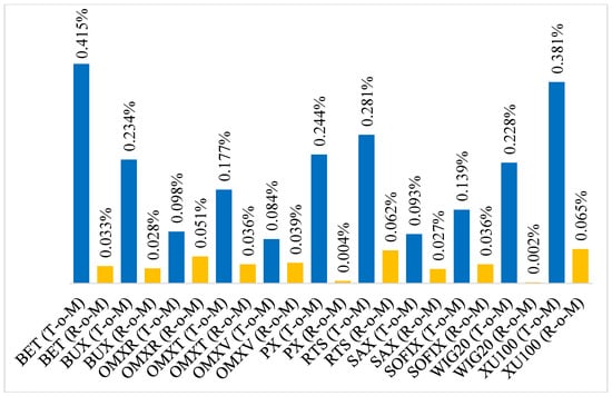
Figure 1.
Comparison of average daily returns—Turn of the month window (1+1).
Table 2 shows the results of statistical significance tests for the turn of the month window (1+1). Parametric two-sample t-test and non-parametric Wilcoxon rank-sum test are both included. However, according to the Jarque-Bera test (Appendix A—Table A1), all of the data analyzed return series are non-normally distributed, which means that the non-parametric Wilcoxon rank-sum test should be more robust (histograms for selected data series can be found in Appendix B—Figure A1 and Figure A2). This applies for all of the analyzed alternatives of the turn of the month window. However, given the large size of analyzed data samples, and given the existence of the central limit theorem, the results of the parametric two-sample t-test should also have some informative value. Moreover, as shown in Table 2, Table 3 and Table 4, there are only two cases when the two-sample t-test and the Wilcoxon rank-sum test provide meaningfully different results (OMXV and WIG 20 for the Turn of the month window (3+3)). At a significance level of α = 0.01, the Turn of the month effect for the (1+1) T-o-M window is statistically significant in six cases (BET, BUX, OMXT, PX, WIG 20, XU 100). At α = 0.1, it is statistically significant in two more cases (OMXV, RTS).
Table 2.
Results of the statistical significance tests—Turn of the month window (1+1).
Table 3.
Results of the statistical significance tests—Turn of the month window (2+2).
Table 4.
Results of the statistical significance tests—Turn of the month window (3+3).
After expanding the turn of the month window to first two and last two trading days of a month (2+2), the results are still very interesting, although the difference in average returns is lower when compared to the (1+1) window. As shown in Figure 2, in this case, the biggest difference in returns was recorded by Romanian BET (0.258 percentage points) and Turkish XU 100. In both of the cases, the average T-o-M returns were higher than the R-o-M returns. However, there were also two stock markets (Latvian—OMR and Slovak—SAX), where the average R-o-M returns were higher than the average T-o-M returns.
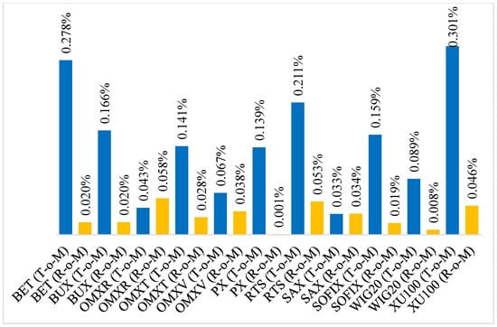
Figure 2.
Comparison of average daily returns—Turn of the month window (2+2).
Table 3 presents the results of the statistical significance tests for the (2+2) turn of the month window. A very strong Turn of the month effect that is statistically significant at α = 0.01 is confirmed in five cases (BET, OMXT, PX, SOFIX, XU 100). At α = 0.05, a statistically significant Turn of the month was also observed in the case of BUX and at α = 0.1 in the case of RTS.
Figure 3 shows the results for the third alternative of the turn of the month window. In this case, the window consists of the first three and last three trading days of a month (3+3). As can be seen, the differences in returns are lower than in the previous two cases. The biggest difference was recorded by Turkish XU 100 (0.223 percentage points) and Romanian BUX (0.176 percentage points). On the Latvian (OMXR) and Slovak (SAX) stock markets, the average T-o-M returns were lower than the average R-o-M returns again.
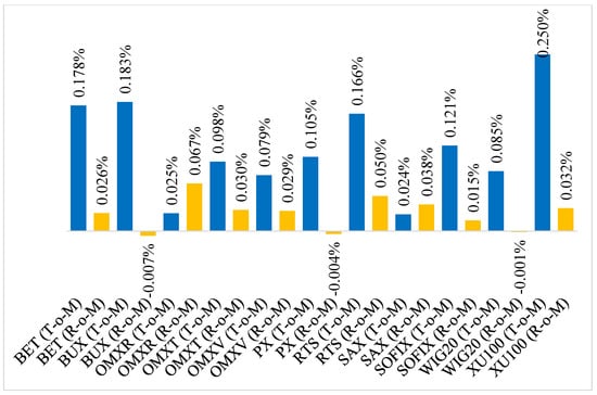
Figure 3.
Comparison of average daily returns—Turn of the month window (3+3).
As shown in Table 4, for the turn of the month window (3+3), the differences between the daily T-o-M returns and R-o-M returns were statistically significant in four cases (BET, BUX, SOFIX, XU 100) at α = 0.01 and in three more cases (OMXT, OMXV, PX) at α = 0.05.
Figure 4 shows the differences in average daily volatilities (alternative 1) calculated as the difference between the highest and lowest trading price recorded during a trading day, divided by the closing price of that trading day. As can be seen, in the case of all four investigated stock markets, the differences between the volatilities recorded over the T-o-M days and volatilities recorded over the R-o-M days is negligible. Moreover, in all of the cases, the R-o-M volatility tends to be slightly higher when compared to the T-o-M volatility. This finding is valid for all three alternatives of the turn of the month window. This finding is surprising, according to the generally accepted theory, higher returns should be connected with higher risk. It means that the stock markets behave counterintuitively, as even on stock markets where a statistically significant Turn of the month effect is present in returns, it is not present in volatility.
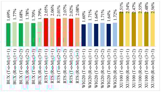
Figure 4.
Comparison of average daily volatilities (alternative 1).
Data that are presented in Figure 4 are also confirmed by the statistical significance tests results that are presented in Table 5. Additionally, for all of the volatility data series applies that they have a non-normal distribution (Appendix A—Table A2), which means that the results of the non-parametric Wilcoxon rank-sum test should be more robust. As can be seen, the difference between the T-o-M and R-o-M daily volatilities is only statistically significant in the case of Hungarian stock index BUX and turn of the month windows (2+2) and (3+3). However, in both cases, the average volatility that was recorded over the T-o-M period is lower than average volatility recorded over the R-o-M period. In other words, the assumption that the statistically significantly higher T-o-M returns should be accompanied by statistically significantly higher T-o-M volatility was not confirmed.
Table 5.
Results of the statistical significance tests—Daily volatilities (alternative 1).
Figure 5 presents the data for daily Garman-Klass volatilities (alternative 2). As can be seen, although the differences between the T-o-M and R-o-M levels of volatility are more noticeable when compared to the first alternative of volatility, the results are consistent and in all of the cases, the average daily volatility was slightly higher during the R-o-M periods.
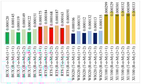
Figure 5.
Comparison of average daily volatilities (alternative 2).
The results of the statistical significance tests for the Garman-Klass volatilities show that statistically significant differences can be seen in the case of BUX (2+2), BUX (3+3), WIG 20 (1+1), and WIG 20 (3+3). What is important, the results of the analysis of Garman-Klass volatility are in line with results of the first alternative of volatility. In the case of all four stock indices and all three turn of the month windows, the average daily volatility is higher during the R-o-M periods. However, the differences are mostly not statistically significant (Table 6).
Table 6.
Results of the statistical significance tests—Daily volatilities (alternative 2).
5. Discussion
The results presented in the previous chapter show that a statistically significant Turn of the month effect could be found on the CEE region stock markets. However, there are several exemptions, as our results did not confirm the presence of a statistically significant Turn of the month effect on the Slovak (SAX) and Latvian (OMXR) stock markets. As a result, Hypothesis 1 (The Turn of the month effect is present on stock markets of the CEE region countries, as the returns recorded during the ToM periods are statistically significantly higher when compared to returns recorded during the RoM periods.) can be confirmed for nine out of 11 investigated stock markets.
These results are in line with some previous studies that concluded the presence of the Turn of the month effect on some of the CEE region stock markets (Heininen and Puttonen 2008; Kayacetin and Lekpek 2016; Arendas and Bukoven 2017). According to Heininen and Puttonen, in Croatia, Hungary, Poland, Romania, Russia, and Slovenia, 85% of monthly returns were recorded during the turn of the month period, between January 1997 and February 2008. Kayacetin and Lekpek confirmed a strong Turn of the month effect on the Turkish stock market, during the 1988–2014 time period. Their turn of the month window included the last and the first two trading days of each month, with an average daily return of 0.46%. Over the remaining days, a return of only 0.09% was recorded. Arendas and Bukoven discovered a strong Turn of the month effect on the Czech stock market during the 1997–2016 period.
While on all the other stock markets, even in the case that the differences were not statistically significant, the average T-o-M returns were higher than the average R-o-M returns for all three alternatives of turn of the month windows, the (2+2) and (3+3) windows for OMXR and the (3+3) window for SAX recorded average R-o-M returns higher when compared to the average T-o-M returns. The tendency of the Slovak stock market to behave differently in comparison to the majority of stock markets in the CEE region was confirmed by numerous researchers, including (Arendas and Chovancova 2016; Olbrys and Majewska 2016; Carausu et al. 2018). This fact is often explained by its lower level of development, insufficient liquidity, and very low market capitalization.
It is also possible to observe an unusual behavior of the Turn of the month effect on the Bulgarian stock market that is represented by SOFIX. While for all of the other stock indices, the p-values tended to increase (or at least stagnate) along expanding turn of the month window, SOFIX behaved in an exactly opposite way. While for the (1+1) window, the differences between the T-o-M and R-o-M windows were not statistically significant, with a p-value of 0.1505, for the (2+2) window the p-value was 0.0037, and for the (3+3) window it was 0.0029. However, the explanation of this behavior will take a more detailed study that directly focuses on specifics of the Bulgarian stock market.
The results also show that, in some of the cases, the differences in T-o-M and R-o-M returns are significant enough to be exploited by an investment strategy. Vasileiou (2018) proposed an investment strategy of holding stocks during the T-o-M windows and keeping the money on a bank account that provides no interest during the rest of the month. During the investigated time periods, this very simple investment strategy would be able to beat a buy & hold investment strategy in the case of the (3+3) T-o-M windows on the Hungarian, Czech, and Polish stock market, as these markets recorded negative average daily returns during the R-o-M periods. Kunkel and Compton (1998) developed a similar strategy, based on switching between the stock market (during the T-o-M periods) and the money market (during the R-o-M periods). Obviously, this investment strategy would also be able to beat the market performance in the case of the Hungarian, Czech, and Polish stock market, due to negative R-o-M returns. Moreover, this strategy provides some potential to also outperform on other markets, especially those with low R-o-M returns (for example, Romania and Bulgaria). However, probably not in the current environment of extremely low interest rates that suppress the money market returns significantly.
It is also possible to note that the observed results are in a contradiction to the efficient markets theory (Fama 1965), according to which the stock prices always reflect all of the important information, thus it is impossible to outperform the market while using technical analysis and market timing. As a result, the presence of an exploitable calendar anomaly, in this case the Turn of the month effect means that the impacted stock market cannot be regarded as efficient.
The most surprising results are related to the testing of the Turn of the month effect in stock market volatilities. In all of the four investigated cases (BUX, RTS, WIG 20, XU 100), although a statistically significant Turn of the month effect in returns was confirmed, the volatility recorded over the T-o-M periods was not statistically significantly higher than the volatility recorded over the R-o-M periods. The average daily volatilities were similar and in all of the cases slightly higher during the R-o-M periods. As a result, Hypothesis 2 (on investigated stock markets, the statistically significantly higher returns recorded over the ToM periods are accompanied by volatilities that are statistically significantly higher when compared to volatilities recorded over the RoM periods) can be completely rejected. This is a very interesting finding, as it is in a direct contradiction to the generally accepted financial markets rule that higher returns are accompanied by higher risk.
Author Contributions
Conceptualization, P.A.; formal analysis, P.A. and J.K.; investigation, P.A. and J.K.; methodology, P.A.; validation, J.K.; writing—original draft preparation, P.A.; writing—review and editing, J.K.
Funding
This paper is an outcome of the science project VEGA (1/0257/18), VEGA (1/0009/17) and VEGA (1/0613/18).
Conflicts of Interest
The authors declare no conflict of interest.
Appendix A
Table A1.
Descriptive statistics—returns.
Table A1.
Descriptive statistics—returns.
| Data | Observ. | Max. | Min. | Average | Jarque-Bera | Prob. |
|---|---|---|---|---|---|---|
| BET (1+1) R-o-M | 4049 | 0.1569 | −0.1122 | 0.0003 | 26,166.14 | 0 |
| BET (1+1) T-o-M | 432 | 0.0950 | −0.0421 | 0.0042 | 569.33 | 0 |
| BET (2+2) R-o-M | 3617 | 0.1569 | −0.1122 | 0.0002 | 25,263.62 | 0 |
| BET (2+2) T-o-M | 864 | 0.0950 | −0.0776 | 0.0028 | 1248.52 | 0 |
| BET (3+3) R-o-M | 3185 | 0.1569 | −0.1122 | 0.0003 | 22,517.77 | 0 |
| BET (3+3) T-o-M | 1296 | 0.0950 | −0.1068 | 0.0018 | 2940.94 | 0 |
| BUX (1+1) R-o-M | 4515 | 0.1408 | −0.1188 | 0.0003 | 8716.05 | 0 |
| BUX (1+1) T-o-M | 480 | 0.0573 | −0.0452 | 0.0023 | 45.81 | 0 |
| BUX (2+2) R-o-M | 4035 | 0.1408 | −0.1188 | 0.0002 | 8653.64 | 0 |
| BUX (2+2) T-o-M | 960 | 0.0738 | −0.0477 | 0.0017 | 159.50 | 0 |
| BUX (3+3) R-o-M | 3555 | 0.1126 | −0.1188 | −0.0001 | 5660.66 | 0 |
| BUX (3+3) T-o-M | 1440 | 0.1408 | −0.0477 | 0.0018 | 3082.05 | 0 |
| OMXR (1+1) R-o-M | 4328 | 0.1230 | −0.1368 | 0.0005 | 45,093.82 | 0 |
| OMXR (1+1) T-o-M | 456 | 0.0759 | −0.1220 | 0.0010 | 7250.06 | 0 |
| OMXR (2+2) R-o-M | 3872 | 0.1230 | −0.1368 | 0.0006 | 43,322.12 | 0 |
| OMXR (2+2) T-o-M | 912 | 0.0776 | −0.1220 | 0.0004 | 9489.82 | 0 |
| OMXR (3+3) R-o-M | 3416 | 0.1230 | −0.1368 | 0.0007 | 38,782.96 | 0 |
| OMXR (3+3) T-o-M | 1368 | 0.0776 | −0.1220 | 0.0003 | 14,224.45 | 0 |
| OMXT (1+1) R-o-M | 4336 | 0.1286 | −0.0680 | 0.0004 | 23,743.65 | 0 |
| OMXT (1+1) T-o-M | 456 | 0.0501 | −0.0422 | 0.0018 | 362.79 | 0 |
| OMXT (2+2) R-o-M | 3880 | 0.1286 | −0.0680 | 0.0003 | 23,604.25 | 0 |
| OMXT (2+2) T-o-M | 912 | 0.0501 | −0.0558 | 0.0014 | 928.31 | 0 |
| OMXT (3+3) R-o-M | 3424 | 0.1286 | −0.0680 | 0.0003 | 23,011.80 | 0 |
| OMXT (3+3) T-o-M | 1368 | 0.0501 | −0.0558 | 0.0010 | 1221.10 | 0 |
| OMXV (1+1) R-o-M | 4312 | 0.1163 | −0.1125 | 0.0004 | 100,522.60 | 0 |
| OMXV (1+1) T-o-M | 456 | 0.0304 | −0.0601 | 0.0008 | 739.34 | 0 |
| OMXV (2+2) R-o-M | 3856 | 0.1163 | −0.1125 | 0.0004 | 93,131.35 | 0 |
| OMXV (2+2) T-o-M | 912 | 0.0501 | −0.0971 | 0.0007 | 8146.88 | 0 |
| OMXV (3+3) R-o-M | 3400 | 0.1163 | −0.1125 | 0.0003 | 91,128.62 | 0 |
| OMXV (3+3) T-o-M | 1368 | 0.0501 | −0.0971 | 0.0008 | 9452.05 | 0 |
| PX (1+1) R-o-M | 4538 | 0.1316 | −0.1494 | 0.0000 | 31,730.44 | 0 |
| PX (1+1) T-o-M | 480 | 0.0620 | −0.0409 | 0.0024 | 106.10 | 0 |
| PX (2+2) R-o-M | 4058 | 0.1316 | −0.1494 | 0.0000 | 31,518.89 | 0 |
| PX (2+2) T-o-M | 960 | 0.0917 | −0.0541 | 0.0014 | 897.24 | 0 |
| PX (3+3) R-o-M | 3578 | 0.1173 | −0.1494 | 0.0000 | 24,076.20 | 0 |
| PX (3+3) T-o-M | 1440 | 0.1316 | −0.0541 | 0.0011 | 6998.43 | 0 |
| RTS (1+1) R-o-M | 4521 | 0.2239 | −0.1910 | 0.0006 | 13,164.68 | 0 |
| RTS (1+1) T-o-M | 480 | 0.1683 | −0.1201 | 0.0028 | 2111.88 | 0 |
| RTS (2+2) R-o-M | 4041 | 0.2239 | −0.1910 | 0.0005 | 11,089.39 | 0 |
| RTS (2+2) T-o-M | 960 | 0.1781 | −0.1201 | 0.0021 | 4454.55 | 0 |
| RTS (3+3) R-o-M | 1440 | 0.1781 | −0.1201 | 0.0017 | 4252.29 | 0 |
| RTS (3+3) T-o-M | 3561 | 0.2239 | −0.1910 | 0.0005 | 10,915.61 | 0 |
| SAX (1+1) R-o-M | 4404 | 0.1261 | −0.1377 | 0.0003 | 33,200.63 | 0 |
| SAX (1+1) T-o-M | 480 | 0.0511 | −0.0844 | 0.0009 | 1422.10 | 0 |
| SAX (2+2) R-o-M | 3924 | 0.0955 | −0.1377 | 0.0003 | 24,408.79 | 0 |
| SAX (2+2) T-o-M | 960 | 0.1261 | −0.0913 | 0.0003 | 8045.54 | 0 |
| SAX (3+3) R-o-M | 3444 | 0.0955 | −0.1085 | 0.0004 | 11,268.57 | 0 |
| SAX (3+3) T-o-M | 1440 | 0.1261 | −0.1377 | 0.0002 | 19,033.62 | 0 |
| SOFIX (1+1) R-o-M | 3784 | 0.0756 | −0.1074 | 0.0004 | 14,788.46 | 0 |
| SOFIX (1+1) T-o-M | 408 | 0.0875 | −0.0679 | 0.0014 | 1821.45 | 0 |
| SOFIX (2+2) R-o-M | 3376 | 0.0756 | −0.1074 | 0.0002 | 14,517.77 | 0 |
| SOFIX (2+2) T-o-M | 816 | 0.0875 | −0.0679 | 0.0016 | 2195.79 | 0 |
| SOFIX (3+3) R-o-M | 2968 | 0.0756 | −0.1074 | 0.0002 | 13,287.55 | 0 |
| SOFIX (3+3) T-o-M | 1224 | 0.0875 | −0.0791 | 0.0012 | 3294.55 | 0 |
| WIG20 (1+1) R-o-M | 4526 | 0.0850 | −0.0925 | 0.0000 | 1509.32 | 0 |
| WIG20 (1+1) T-o-M | 480 | 0.0635 | −0.0511 | 0.0023 | 57.14 | 0 |
| WIG20 (2+2) R-o-M | 4046 | 0.0850 | −0.0925 | 0.0001 | 1428.46 | 0 |
| WIG20 (2+2) T-o-M | 960 | 0.0695 | −0.0660 | 0.0009 | 155.12 | 0 |
| WIG20 (3+3) R-o-M | 3566 | 0.0850 | −0.0925 | 0.0000 | 1214.28 | 0 |
| WIG20 (3+3) T-o-M | 1440 | 0.0773 | −0.0660 | 0.0008 | 358.03 | 0 |
| XU100 (1+1) R-o-M | 4525 | 0.1945 | −0.1811 | 0.0006 | 10,682.99 | 0 |
| XU100 (1+1) T-o-M | 480 | 0.1515 | −0.1249 | 0.0038 | 1202.94 | 0 |
| XU100 (2+2) R-o-M | 4045 | 0.1945 | −0.1811 | 0.0005 | 10,032.85 | 0 |
| XU100 (2+2) T-o-M | 960 | 0.1515 | −0.1249 | 0.0030 | 1990.83 | 0 |
| XU100 (3+3) R-o-M | 3565 | 0.1864 | −0.1811 | 0.0003 | 6590.06 | 0 |
| XU100 (3+3) T-o-M | 1440 | 0.1945 | −0.1249 | 0.0025 | 5335.24 | 0 |
Table A2.
Descriptive statistics—volatilities.
Table A2.
Descriptive statistics—volatilities.
| Data | Observ. | Max. | Min. | Average | Jarque-Bera | Prob. |
|---|---|---|---|---|---|---|
| BUX (1+1) R-o-M (HL) | 4515 | 0.1766 | 0.0000 | 0.0177 | 128,075.60 | 0 |
| BUX (1+1) T-o-M (HL) | 480 | 0.0645 | 0.0041 | 0.0169 | 590.34 | 0 |
| BUX (2+2) R-o-M (HL) | 4035 | 0.1766 | 0.0000 | 0.0178 | 122,576.80 | 0 |
| BUX (2+2) T-o-M (HL) | 960 | 0.0645 | 0.0041 | 0.0168 | 1191.09 | 0 |
| BUX (3+3) R-o-M (HL) | 3555 | 0.1766 | 0.0000 | 0.0179 | 112,319.30 | 0 |
| BUX (3+3) T-o-M (HL) | 1440 | 0.0810 | 0.0041 | 0.0170 | 3390.14 | 0 |
| RTS (1+1) R-o-M (HL) | 4521 | 0.2767 | 0.0000 | 0.0206 | 231,355.50 | 0 |
| RTS (1+1) T-o-M (HL) | 480 | 0.1427 | 0.0006 | 0.0205 | 6054.83 | 0 |
| RTS (2+2) R-o-M (HL) | 4041 | 0.2767 | 0.0000 | 0.0207 | 213,977.40 | 0 |
| RTS (2+2) T-o-M (HL) | 960 | 0.1573 | 0.0006 | 0.0201 | 15,253.23 | 0 |
| RTS (3+3) R-o-M (HL) | 3561 | 0.2767 | 0.0000 | 0.0208 | 200,790.60 | 0 |
| RTS (3+3) T-o-M (HL) | 1440 | 0.1573 | 0.0006 | 0.0202 | 16,600.13 | 0 |
| WIG20 (1+1) R-o-M (HL) | 4526 | 0.1403 | 0.0035 | 0.0171 | 41,457.13 | 0 |
| WIG20 (1+1) T-o-M (HL) | 480 | 0.0538 | 0.0048 | 0.0160 | 355.79 | 0 |
| WIG20 (2+2) R-o-M (HL) | 4046 | 0.1403 | 0.0035 | 0.0171 | 40,513.95 | 0 |
| WIG20 (2+2) T-o-M (HL) | 960 | 0.0612 | 0.0037 | 0.0164 | 843.59 | 0 |
| WIG20 (3+3) R-o-M (HL) | 3566 | 0.1403 | 0.0035 | 0.0172 | 38,170.42 | 0 |
| WIG20 (3+3) T-o-M (HL) | 1440 | 0.0612 | 0.0037 | 0.0164 | 1200.64 | 0 |
| XU100 (1+1) R-o-M (HL) | 4525 | 0.2233 | 0.0000 | 0.0254 | 41,770.67 | 0 |
| XU100 (1+1) T-o-M (HL) | 480 | 0.1494 | 0.0000 | 0.0251 | 4625.07 | 0 |
| XU100 (2+2) R-o-M (HL) | 4045 | 0.2233 | 0.0000 | 0.0255 | 37,845.86 | 0 |
| XU100 (2+2) T-o-M (HL) | 960 | 0.1494 | 0.0000 | 0.0247 | 8374.23 | 0 |
| XU100 (3+3) R-o-M (HL) | 3565 | 0.2233 | 0.0000 | 0.0256 | 31,016.39 | 0 |
| XU100 (3+3) T-o-M (HL) | 1440 | 0.1796 | 0.0000 | 0.0248 | 15,708.37 | 0 |
| BUX (1+1) R-o-M (GK) | 4515 | 0.0139 | 0.0000 | 0.0001 | 93,778,956.00 | 0 |
| BUX (1+1) T-o-M (GK) | 480 | 0.0010 | 0.0000 | 0.0001 | 2981.27 | 0 |
| BUX (2+2) R-o-M (GK) | 4035 | 0.0139 | 0.0000 | 0.0001 | 72,960,991.00 | 0 |
| BUX (2+2) T-o-M (GK) | 960 | 0.0015 | 0.0000 | 0.0001 | 22,038.93 | 0 |
| BUX (3+3) R-o-M (GK) | 3555 | 0.0139 | 0.0000 | 0.0002 | 55,999,012.00 | 0 |
| BUX (3+3) T-o-M (GK) | 1440 | 0.0019 | 0.0000 | 0.0001 | 89,751.11 | 0 |
| RTS (1+1) R-o-M (GK) | 4521 | 0.0299 | 0.0000 | 0.0002 | 571,000,000.00 | 0 |
| RTS (1+1) T-o-M (GK) | 480 | 0.0042 | 0.0000 | 0.0002 | 95,374.30 | 0 |
| RTS (2+2) R-o-M (GK) | 4041 | 0.0299 | 0.0000 | 0.0002 | 464,000,000.00 | 0 |
| RTS (2+2) T-o-M (GK) | 960 | 0.0042 | 0.0000 | 0.0002 | 221,552.20 | 0 |
| RTS (3+3) R-o-M (GK) | 1440 | 0.0042 | 0.0000 | 0.0002 | 331,714.90 | 0 |
| RTS (3+3) T-o-M (GK) | 3561 | 0.0299 | 0.0000 | 0.0002 | 341,000,000.00 | 0 |
| WIG20 (1+1) R-o-M (GK) | 4526 | 0.0054 | 0.0000 | 0.0001 | 4,591,646.00 | 0 |
| WIG20 (1+1) T-o-M (GK) | 480 | 0.0010 | 0.0000 | 0.0001 | 3590.90 | 0 |
| WIG20 (2+2) R-o-M (GK) | 4046 | 0.0054 | 0.0000 | 0.0001 | 3,771,200.00 | 0 |
| WIG20 (2+2) T-o-M (GK) | 960 | 0.0011 | 0.0000 | 0.0001 | 8880.60 | 0 |
| WIG20 (3+3) R-o-M (GK) | 1440 | 0.0012 | 0.0000 | 0.0001 | 16,561.43 | 0 |
| WIG20 (3+3) T-o-M (GK) | 3566 | 0.0054 | 0.0000 | 0.0001 | 2,997,413.00 | 0 |
| XU100 (1+1) R-o-M (GK) | 4525 | 0.0179 | 0.0000 | 0.0003 | 4,427,421.00 | 0 |
| XU100 (1+1) T-o-M (GK) | 480 | 0.0066 | 0.0000 | 0.0003 | 49,526.45 | 0 |
| XU100 (2+2) R-o-M (GK) | 4045 | 0.0179 | 0.0000 | 0.0003 | 4,357,226.00 | 0 |
| XU100 (2+2) T-o-M (GK) | 960 | 0.0071 | 0.0000 | 0.0003 | 107,348.80 | 0 |
| XU100 (3+3) R-o-M (GK) | 3565 | 0.0179 | 0.0000 | 0.0003 | 4,254,954.00 | 0 |
| XU100 (3+3) T-o-M (GK) | 1440 | 0.0108 | 0.0000 | 0.0003 | 418,241.10 | 0 |
Appendix B

Figure A1.
Histograms and descriptive statistics for data samples with highest difference between average T-o-M and R-o-M returns.
Figure A1.
Histograms and descriptive statistics for data samples with highest difference between average T-o-M and R-o-M returns.


Figure A2.
Histograms and descriptive statistics for data samples with lowest difference between average T-o-M and R-o-M returns References.
Figure A2.
Histograms and descriptive statistics for data samples with lowest difference between average T-o-M and R-o-M returns References.

References
- Aggarwal, Raj, and John D. Schatzberg. 1997. Day of the week effects, information seasonality, and higher moments of security returns. Journal of Economics and Business 49: 1–20. [Google Scholar] [CrossRef]
- Agrawal, Anup, and Kishore Tandon. 1994. Anomalies or illusions? Evidence from stock markets in eighteen countries. Journal of International Money and Finance 13: 83–106. [Google Scholar] [CrossRef]
- Andrade, Sandro C., Vidhi Chhaochharia, and Michael E. Fuerst. 2013. “Sell in May and Go Away” Just Won’t Go Away. Financial Analysts Journal 69: 94–105. [Google Scholar] [CrossRef]
- Arendas, Peter. 2017. The Halloween Effect on the Agricultural Commodities Markets. Agricultural Economics 63: 441–48. [Google Scholar] [CrossRef]
- Arendas, Peter, and Jan Bukoven. 2017. Turn of the month effect on the Prague stock exchange. Paper presented at the 8th International Scientific Conference, Finance and Performance of Firms in Science, Education and Practice, Zlin, Czech Republic, April 26–27. [Google Scholar]
- Arendas, Peter, and Bozena Chovancova. 2016. Central and Eastern European Share Markets and the Halloween Effect. Montenegrin Journal of Economics 12: 61–71. [Google Scholar] [CrossRef]
- Arendas, Peter, Viera Malacka, and Maria Schwarzova. 2018. A Closer Look at the Halloween Effect: The Case of the Dow Jones Industrial Average. International Journal of Financial Studies 6: 42. [Google Scholar] [CrossRef]
- Ariel, Robert A. 1987. A Monthly Effect in Stock Returns. Journal of Financial Economics 18: 621–28. [Google Scholar] [CrossRef]
- Ariel, Robert A. 1990. High Stock Returns before Holidays: Existence and Evidence on Possible Causes. The Journal of Finance 45: 1611–26. [Google Scholar] [CrossRef]
- Aziz, Tariq, and Valeed A. Ansari. 2017. The Turn of the Month Effect in Asia-Pacific Markets: New Evidence. Global Business Review 19: 214–26. [Google Scholar] [CrossRef]
- Borowski, Krzysztof. 2015. Analysis of selected seasonality effects in market of barley, canola, rough rice, soybean oil and soybean meal future contracts. Journal of Economics and Management 21: 73–89. [Google Scholar]
- Bouman, Sven, and Ben Jacobsen. 2002. The Halloween indicator, “sell in May and go away”: Another puzzle. American Economic Review 92: 1618–35. [Google Scholar] [CrossRef]
- Brusa, Jorge, and Pu Liu. 2004. The Day-of-the-Week and the Week-of-the-Month Effects: An Analysis of Investors’ Trading Activities. Review of Quantitative Finance and Accounting 23: 19–30. [Google Scholar] [CrossRef]
- Burakov, Dmitry, and Max Freidin. 2018. Is the Halloween Effect Present on the Markets for Agricultural Commodities? Agris on-line Papers in Economics and Informatics 10: 23–32. [Google Scholar] [CrossRef]
- Burakov, Dmitry, Max Freidin, and Yuriy Solovyev. 2018. The halloween effect on energy markets: An empirical study. International Journal of Energy Economics and Policy 8: 121–26. [Google Scholar] [CrossRef]
- Burnett, John E. 2017. Liquidity and investor confidence in the turn-of-the-month regularity. Applied Economics Letters 24: 273–78. [Google Scholar] [CrossRef]
- Cadsby, Charles, and Mitchell Ratner. 1992. Turn-of-month and pre-holiday effects on stock returns: Some international evidence. Journal of Banking & Finance 16: 497–509. [Google Scholar] [CrossRef]
- Caporale, Guglielmo M., and Alex Plastun. 2017. Calendar anomalies in the Ukrainian stock market. Investment Management and Financial Innovations 14: 104–14. [Google Scholar] [CrossRef]
- Carausu, Dimitru N., Bogdan F. Filip, Elena Cigu, and Carmen Toderascu. 2018. Contagion of Capital Markets in CEE Countries: Evidence from Wavelet Analysis. Emerging Markets Finance & Trade 54: 618–41. [Google Scholar] [CrossRef]
- Chen, Jun, Bart Frijns, Ivan Indriawan, and Haodong Ren. 2018. Turn of the Month effect in the New Zealand stock market. New Zealand Economic Papers, 1–19. [Google Scholar] [CrossRef]
- Dichtl, Hubert, and Wolfgang Drobetz. 2015. Sell in May and Go Away: Still Good Advice for Investors? International Review of Financial Analysis 38: 29–43. [Google Scholar] [CrossRef]
- Fama, Eugene F. 1965. Random Walks in Stock Market Prices. Financial Analysts Journal 21: 55–59. [Google Scholar] [CrossRef]
- Ferreira, Paulo. 2018. What guides Central and Eastern European stock markets? A view from detrended methodologies. Post-Communist Economies 30: 1–15. [Google Scholar] [CrossRef]
- Giovanis, Eleftherios. 2009. Calendar Effects in Fifty-five Stock Market Indices. Global Journal of Finance and Management 1: 75–98. [Google Scholar]
- Giovanis, Eleftherios. 2014. The Turn-of-the-Month-Effect: Evidence from Periodic Generalized Autoregressive Conditional Heteroskedasticity (PGARCH) Model. International Journal of Economic Sciences and Applied Research 7: 43–61. [Google Scholar] [CrossRef]
- Heininen, Polina, and Puttonen Vesa. 2008. Stock Market Efficiency In The Transition Economies Through The Lens Of Calendar Anomalies. Paper presented at EACES 10th Bi-Annual Conference Patterns of Transition and New Approaches to Comparative Eoconomics, Higher School of Economics, Moscow, Russia, August 28–30. [Google Scholar]
- Horvath, Roman, Stefan Lyocsa, and Eduard Baumohl. 2018. Stock market contagion in Central and Eastern Europe: Unexpected volatility and extreme co-exceedance. The European Journal of Finance 24: 391–412. [Google Scholar] [CrossRef]
- Kayacetin, Volkan, and Senad Lekpek. 2016. Turn-of-the-month effect: New evidence from an emerging stock market. Finance Research Letters 18: 142–57. [Google Scholar] [CrossRef]
- Keim, Donald B. 1983. Size-Related Anomalies and Stock Return Seasonality: Further Empirical Evidence. Journal of Financial Economics 12: 13–32. [Google Scholar] [CrossRef]
- Kunkel, Robert A., and William S. Compton. 1998. A tax-free exploitation of the turn-of-the-month effect: C.R.E.F. Financial Services Review 7: 11–23. [Google Scholar] [CrossRef]
- Kunkel, Robert, William S. Compton, and Scott B. Beyer. 2003. The turn-of-the-month effect still lives: The international evidence. International Review of Financial Analysis 12: 207–21. [Google Scholar] [CrossRef]
- Lakonishok, Josef, and Seymour Smidt. 1988. Are Seasonal Anomalies Real? A Ninety-Year Perspective. The Review of Financial Studies 1: 403–25. [Google Scholar] [CrossRef]
- Liu, Lan. 2013. The Turn-Of-The-Month Effect In The S&P 500 (2001–2011). Journal of Business & Economics Research 11: 269–76. [Google Scholar] [CrossRef]
- Lo, Andrew W. 2004. The Adaptive Markets Hypothesis: Market Efficiency from an Evolutionary Perspective. Journal of Portfolio Management 30: 15–29. [Google Scholar] [CrossRef]
- Maher, Daniela, and Anokhi Parikh. 2013. The turn of the month effect in India: A case of large institutional trading patterns as a source of higher liquidity. International Review of Financial Analysis 28: 57–69. [Google Scholar] [CrossRef]
- McConnell, John J., and Wei Xu. 2008. Equity Returns at the Turn of the Month. Financial Analysts Journal 64: 49–64. [Google Scholar] [CrossRef]
- Milonas, Nikolaos T. 1991. Measuring Seasonalities in Commodity Markets and the Half-Month Effect. The Journal of Futures Markets 11: 331–45. [Google Scholar] [CrossRef]
- Moller, Nicholas, and Shlomo Zilca. 2008. The evolution of the January effect. Journal of Banking & Finance 32: 447–57. [Google Scholar] [CrossRef]
- Molnar, Peter. 2012. Properties of range-based volatility estimators. International Review of Financial Analysis 23: 20–29. [Google Scholar] [CrossRef]
- Nikkinen, Jussi, Sahlstrom Petri, Takko Karri, and Janne Aijo. 2009. Turn-of-the-month and Intramonth Anomalies and U.S. Macroeconomic News Announcements on the Thinly Traded Finnish Stock Market. International Journal of Economics and Finance 1: 3–11. [Google Scholar] [CrossRef]
- Ogden, Joseph P. 1990. Turn-of-Month Evaluations of Liquid Profits and Stock Returns: A Common Explanation for the Monthly and January Effects. The Journal of Finance 45: 1259–72. [Google Scholar] [CrossRef]
- Olbrys, Joanna, and Elzbieta Majewska. 2016. Crisis periods and contagion effects in the CEE stock markets: The influence of the 2007 US subprime crisis. International Journal of Computational Economics and Econometrics 6: 124–37. [Google Scholar] [CrossRef]
- Philpot, James, and Craig A. Peterson. 2011. A brief history and recent developments in day-of-the-week effect literature. Managerial Finance 37: 808–16. [Google Scholar] [CrossRef]
- Roberts, Harry. 1967. Statistical Versus Clinical Prediction of the Stock Market. Chicago: CRSP University of Chicago. [Google Scholar]
- Vasileiou, Evangelos. 2018. Is the turn of the month effect an “abnormal normality”? Controversial findings, new patterns and... hidden signs(?). Research in International Business and Finance 44: 153–75. [Google Scholar] [CrossRef]
- Vychytilova, Jana. 2018. Stock market development beyond the GFC: The case of V4 countries. Journal of Competitiveness 10: 149–63. [Google Scholar] [CrossRef]
- Wachtel, Sidney B. 1942. Certain Observations on Seasonal Movements in Stock Prices. The Journal of Business of the University of Chicago 15: 184–93. [Google Scholar] [CrossRef]
- Zaremba, Adam. 2019. Trading costs, short sale constraints, and the performance of stock market anomalies in Emerging Europe. Economic Research-Ekonomska Istrazivanja 32: 403–22. [Google Scholar] [CrossRef]


© 2019 by the authors. Licensee MDPI, Basel, Switzerland. This article is an open access article distributed under the terms and conditions of the Creative Commons Attribution (CC BY) license (http://creativecommons.org/licenses/by/4.0/).