The Laws of Motion of the Broker Call Rate in the United States

Abstract

In this paper, which is the third installment of the author’s trilogy on margin loan pricing, we analyze 1367 monthly observations of the U.S. broker call money rate, e.g., the interest rate at which stockbrokers can borrow to fund their margin loans to retail clients. We describe the basic features and mean-reverting behavior of this series and juxtapose the empirically-derived laws of motion with the author’s prior theories of margin loan pricing (Garivaltis 2019a, 2019b). This allows us to derive stochastic differential equations that govern the evolution of the margin loan interest rate and the leverage ratios of sophisticated brokerage clients (namely, continuous-time Kelly gamblers). Finally, we apply Merton’s (1974) arbitrage theory of corporate liability pricing to study theoretical constraints on the risk premia that could be generated in the market for call money. Apparently, if there is no arbitrage in the U.S. financial markets, the implication is that the total volume of call loans must constitute north of $70\%$ of the value of all leveraged portfolios.

1. Introduction

This paper adds to the literature on margin loan behavior in the stock markets of developed economies by estimating some mean-reverting stochastic processes for the U.S. broker call money rate in both discrete and continuous time. The broker call rate is the interest rate that banks and other financial institutions charge for short term credits to investment brokerages, who in turn loan the money to their clients (at a markup) in the form of margin debt.

We combine these purely empirical specifications with the author’s prior theoretical formulas on margin loan pricing (cf. with Garivaltis 2019a, 2019b) in order to derive empirical stochastic processes that govern the time series for brokers’ margin loan interest rates and the (unobservable) leverage ratios of their most well-heeled and sophisticated clients (e.g., continuous-time Kelly gamblers). Thus, the present work enhances the literature by offering hybrid empirical/theoretical statistical models of certain financial time series (e.g., the margin loan interest rates charged by brokers to their retail clients) for which the existing set of historical data is either nonexistent or very spotty, at best.

To be more specific, our particular contribution amounts to combining the empirical time series for the U.S. broker call rate with the following two theoretical relationships derived by the author in his prior work (e.g., in the first two installments of his Margin Loan Trilogy ).

■

The instantaneous monopoly price of margin loans to Kelly (1956) gamblers:

$$r_L^{*}=\frac{1}{2}{r}_B+\frac{1}{2}\left(\nu -\frac{{\sigma }^2}{2}\right).$$

(1)

■

The negotiated interest rate under instantaneous Nash (1950) Bargaining1 with Kelly gamblers:

$$r_L^{*}=\frac{3}{4}{r}_B+\frac{1}{4}\left(\nu -\frac{{\sigma }^2}{2}\right).$$

(2)

In these formulas, $r_L^{*}$ denotes the (continuously-compounded) margin loan interest rate charged by the broker over the differential time step $\left[t,t+dt\right]$, where $\nu :=\mu -{\sigma }^2/2$ is the asymptotic (or logarithmic) growth rate of the stock market index, $\sigma$ is the annual volatility, and $\mu$ is the annual (arithmetic) drift rate. $r_B$ denotes the broker’s cost of funding (“broker call money rate”) for the duration $\left[t,t+dt\right]$. These formulas are of great interest on account of their simplicity and their practicality; naturally, the broker charges more if the underlying growth opportunity

$$d{S}_t:=\mu dt+\sigma d{W}_t$$

(3)

$$d\left(log{S}_t\right)=\left(\mu -\frac{{\sigma }^2}{2}\right)dt+\sigma d{W}_t,$$

(4)

is more favorable (higher $\nu$, lower $\sigma$). Because all the action (the broker posts a monopoly price, or the principals Nash bargain over both the price and quantity of margin loans) happens over the differential time step $[t,t+dt]$, the formulas apply equally well to a general situation whereby the stock market index $S_t$ is governed by time- and state-dependent parameters $\mu (S_t,t)$ and $\sigma (S_t,t)$. The affine relationships (1) and (2) imply that the net interest margin $r_L^{*}-r_B$ must shrink whenever the broker call rate $r_B$ increases; ceteris paribus, for a 100 basis point fluctuation in the broker call rate, only 50 bps will pass through to the consumer (or 75 bps under Nash Bargaining).

The purpose of this article, then, is to use empirical data to divine the general laws of motion of the U.S. broker call rate $r_B\left(t\right)$, and to study the logical consequences for the random behavior of margin loan interest rates, risk premia, and the leverage ratios of continuous time Kelly gamblers. The U.S. broker call money rate, which is published daily in periodicals like The Wall Street Journal and Investor’s Business Daily, is so-named because stock brokers must be prepared to repay these funds immediately upon “call” from the lending institution.

The paper is organized as follows. Section 2 describes our data set, which consists of some 1367 monthly observations (covering the years 1857–1970) published by the Federal Reserve Bank of St. Louis (FRED). We estimate the mean-reverting (monthly) specification

$$\mathrm{Call}{\mathrm{Rate}}_{t+1}=\underset{\left(0.08\right)}{3.943}+\underset{\left(0.022\right)}{0.597}\times \left(\mathrm{Call}{\mathrm{Rate}}_t-\underset{\left(0.08\right)}{3.943}\right)+2.362\times {ϵ}_t,$$

(5)

and use it to construct a classical method-of-moments estimator of the analogous Ornstein–Uhlenbeck process (or Vasicek model) in continuous time. Inspired by the fact that Bankrate.com reports only the two most recent monthly observations of the broker call rate, we develop some out-of-sample forecasts based on the empirical AR(2) model

$$\mathrm{Call}{\mathrm{Rate}}_{t+1}=\underset{\left(0.112\right)}{1.215}+\underset{\left(0.026\right)}{0.456}·\mathrm{Call}{\mathrm{Rate}}_t+\underset{\left(0.026\right)}{0.235}·\mathrm{Call}{\mathrm{Rate}}_{t-1}+2.297\times {ϵ}_t.$$

(6)

Section 3 juxtaposes the empirical specifications (5) and (6) with the theoretical pricing formula (1) to derive stochastic differential and difference equations that must govern the evolution of the margin loan interest rates charged by stock brokers. As an application, we deduce and simulate the implied law of motion for the leverage ratios of continuous time Kelly gamblers. Finally, Section 4 applies Merton’s (1974) arbitrage theory of corporate liability pricing to derive theoretical constraints on the risk premia that could be generated in the market for call money. Based on Fortune’s (2000) suggestion, we model a situation whereby stock brokers are not willing or able to hedge the default risks of their margin loans; at the same time, they must pledge their customers’ securities as collateral to the banks and financial institutions who lend in the market for call money. This environment generates positive risk premia because the banks are exposed to a credit event whereby the retail client defaults on his margin loan, and the broker in turn defaults on its debt to the banks that (partially) funded the loan. Our numerical work indicates that, in comparing the prevailing (low) U.S. Treasury yields with the broker call rate (which is $4.25\%$ as of this writing), the implied loan-to-value ratios of retail borrowers are north of 70 percent. This is an absurd figure (for one thing, it contradicts U.S. Regulation-T), and it seems to indicate that U.S. banks are earning substantial arbitrage profits on the spread of the call rate over the risk-free rate. Section 5 concludes the paper.

Related Literature

The present paper adds to a substantial and exciting literature that studies the empirical aspects of margin lending by investment brokerages in the United States and other developed economies (most notably, Japan). However, most of these papers concentrate on the regulatory aspects of setting the proper margin requirements, and the consequences that this regulation can have for stock market volatility and asset returns. Thus, the present work offers some unique perspectives and direct insights into empirical margin loan pricing dynamics, insights that are sorely lacking in the existing literature.

Fortune (2001) studies the mechanisms by which margin loans increase the variability of prices in the stock market. Lepetit et al. (2008) construct an interesting empirical study of how European banks’ expansion into fee-based services affected their margin loan pricing during the period 1996–2002. Hirose et al. (2009) examine empirical investor behaviors in the Japanese stock market, wherein margin trading is dominated by small (retail) investors. They conclude that information on the number of margin purchases can be predictive of future asset returns, especially of small-cap stocks over short periods of time. Speaking of the Japanese market, Hardouvelis and Peristiani (1992) find that an increase of the margin requirements in the First Section of the Tokyo Stock Exchange will typically lead to a decline in margin borrowing, trading volume, and the conditional volatility of daily returns. They find that, coincidentally, individual traders who make the most active use of margin loans also seem to be in possession of superior market-timing abilities. More recently, Hardouvelis and Theodossiou (2002) considered asymmetry in the relation between initial margin requirements and stock market volatility across different bull and bear markets. They found that it is preferable (from a regulatory perspective) to lower the margin requirements in bear markets and to raise them in bull markets, so as to prevent pyramiding effects. Watanabe (2002) investigates the autocorrelation of daily returns on the Tokyo Stock Exchange and finds evidence that an increase in margin requirements will correspondingly increase the level of autocorrelation in stock returns. His result contrasts with the empirical findings of Sentana and Wadhwani (1992), who found that margin requirements have no significant effect on the autocorrelation of U.S. stock returns.

2. Broker Call Rate

2.1. Basic Description of the Data

We proceed to analyze $T:=1367$ monthly observations of the broker call money rate (1 January 1857 through 1 November 1970, annual interest rates, in percent) as published by the Federal Reserve Bank of St. Louis’ macrohistory database (FRED). In order to find agreement with the author’s prior work on margin loan pricing (Garivaltis 2019a, 2019b), we must deal with the continuously-compounded annual interest rate, as follows:

$$\begin{array}{c}{y}_t:=\text{Continuously-Compounded}\mathrm{Interest}{\mathrm{Rate}}_t\hfill \\ =100\times log\left(1+\frac{\mathrm{Interest}{\mathrm{Rate}}_t}{100}\right)\hfill \\ =\mathrm{Interest}{\mathrm{Rate}}_t-\frac{{\left(\mathrm{Interest}{\mathrm{Rate}}_t\right)}^2}{200}+\frac{{\left(\mathrm{Interest}{\mathrm{Rate}}_t\right)}^3}{30,000}-\cdots \hfill \end{array}$$

(7)

Figure 1 gives a plot of the time series ${\left(y_t\right)}_{t=1}^T$; the grey bars on the figure indicate National Bureau of Economic Research (NBER) recessions, which have typically corresponded to precipitous declines in the interest rate. The time series exhibits several obvious structural breaks, viz., in the 1870s, the 1900s, and the 1920s. However, the present study focuses most of its attention on the mean-reverting aspects of the U.S. broker call rate; the author plans to study possible hidden (Markovian) regime changes in a future paper. For the sake of smoothing out the choppy appearance of ${\left(y_t\right)}_{t=1}^T$, Figure 2 plots the 12-month simple moving average (SMA) given by

$${\overline{y}}_t:=\frac{1}{12}\sum _{j=0}^{11}{y}_{t-j}.$$

(8)

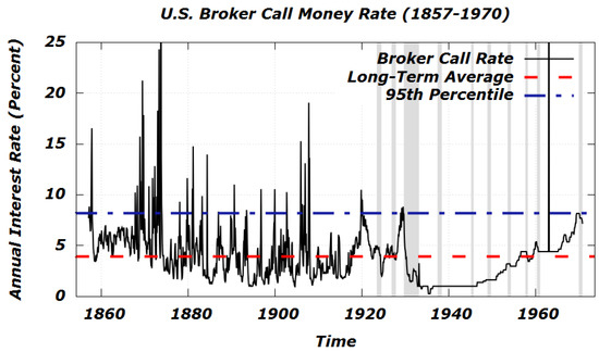
Figure 1. Monthly observations of the U.S. broker call money rate (continuously-compounded, in percent) from 1 January 1857 through 1 November 1970. The grey bars indicate NBER recessions.

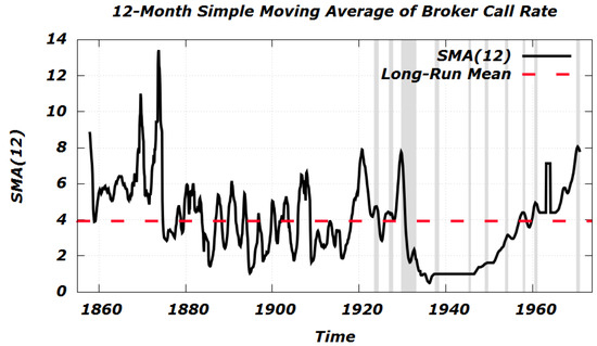
Figure 2. 12-month simple moving average of the broker call rate (in percent). The grey bars indicate National Bureau of Economic Research (NBER) recessions.

Table 1 contains basic descriptive information about the broker call rate; in our sample, the call money rate averaged $3.95\%$, with a standard deviation of $2.95\%$ from its long-run mean. The mean absolute deviation was $1.95\%$. Although at times the broker call rate has spiked to levels as high as $47.8\%$, the historical 95th percentile is a more palatable $8.16\%$.

Table 1. Summary statistics for monthly observations of the U.S. broker call money rate.

Sample Statistic	Value
Observation frequency	Monthly
Number of observations (T)	1367
Time span	114 years
Average	3.95%
Minimum	0.25%
Maximum	47.77%
Standard deviation	2.95%
Coefficient of variation	0.746
Mean absolute deviation	1.95%
Skewness	4.62
5th percentile	1%
50th percentile (median)	3.69%
95th percentile	8.16%

Basic Quantitative Description of the Broker Call Money Rate (1857:01–1970:11).

Figure 3 shows a histogram of the realizations ${\left(y_t\right)}_{t=1}^{1,367}={\left(\mathrm{Call}{\mathrm{Rate}}_t\right)}_{t=1}^{1,367}$. On that score, making use of Gaussian basis functions and a bandwidth of $h:=0.502$, we have the estimated population density function

$$\widehat{f}\left(y\right):=0.000581\times \sum _{t=1}^{1,367}{0.138}^{{\left(y-\mathrm{Call}{\mathrm{Rate}}_t\right)}^2},$$

(9)

which is plotted in Figure 4. To help visualize the internal correlation structure of the call money rate, Figure 5 gives a plot of the sample autocorrelation function

$${\widehat{\rho }}_j:=0.0000843\times \sum _{t=j+1}^{1,367}\left(y_t-3.95\right)\left(y_{t-j}-3.95\right),$$

(10)

where $j\in \left\{0,\dots ,12\right\}$ denotes the number of lags, in months. The sample correlation coefficient for successive monthly observations is ${\widehat{\rho }}_1=59.7\%$. In order to control for any confounding effects that the interim observations $\left(y_{t-j+1},y_{t-j+2},\dots ,y_{t-1}\right)$ could possibly have on the observed relationship between $y_{t-j}$ and $y_t$, Figure 6 supplements the sample correlogram with a 24-month plot of the sample partial autocorrelation function. As illustrated by the figure, the partial autocorrelations start to lose their statistical significance for lags in excess of 12 months.

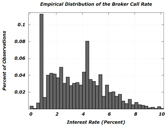
Figure 3. Histogram for the U.S. broker call rate (continuously-compounded, in percent). $\mathrm{Bin}\mathrm{width}:=25\mathrm{basis}\mathrm{points}$; values $>10\%$ are not pictured.

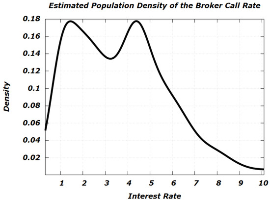
Figure 4. Estimated population density $\widehat{f}\left(y\right)$ for the U.S. broker call rate (Gaussian kernel, $\mathrm{bandwidth}:=0.502$). The modes are $\approx 1.4\%\mathrm{and}4.4\%.$

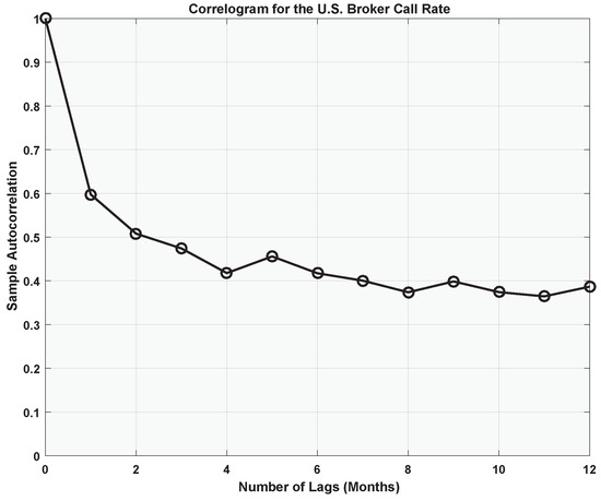
Figure 5. The 12-month sample correlogram for the U.S. broker call rate.

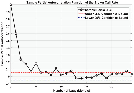
Figure 6. 24-month plot of the sample partial autocorrelation function of the U.S. broker call rate.

2.2. Reversion to the Mean

Drawing some inspiration from the sample autocorrelation function as depicted in Figure 5, we proceed to estimate a stationary first-order autoregressive model of ${\left(y_t\right)}_{t=1}^T$. This amounts to the linear stochastic difference equation

$$\mathrm{Call}{\mathrm{Rate}}_{t+1}=\alpha +\rho ·\mathrm{Call}{\mathrm{Rate}}_t+\sigma {ϵ}_t,$$

(11)

or, equivalently,

$$\left(1-\rho L\right)y_{t+1}=\alpha +\sigma {ϵ}_t,$$

(12)

where L denotes the lag operator. The deep parameters are $\alpha ,\rho ,\mathrm{and}\sigma$, and the stochastic shocks ${\left({ϵ}_t\right)}_{t=1}^T$ are assumed to be unit white noise, e.g., they are serially uncorrelated, $\mathbb{E}\left[{ϵ}_t\right]\equiv 0$, and $\mathrm{Var}\left[{ϵ}_t\right]\equiv 1$. The contemporaneous disturbance ${ϵ}_t$ is assumed to be uncorrelated with $\mathrm{Call}{\mathrm{Rate}}_t$.

Under this terminology, the long-run mean of the (continuously-compounded) interest rate is given by

$$\mu :=\mathbb{E}\left[\mathrm{Call}{\mathrm{Rate}}_t\right]=\frac{\alpha }{1-\rho },$$

(13)

and the stationary variance and standard deviation are equal to

$$v:=\mathrm{Var}\left[\mathrm{Call}{\mathrm{Rate}}_t\right]=\frac{{\sigma }^2}{1-{\rho }^2}$$

(14)

and

$$s:=\mathrm{Std}(\mathrm{Call}{\mathrm{Rate}}_t)=\sqrt{v}=\frac{\sigma }{\sqrt{1-{\rho }^2}}.$$

(15)

Of course, the (aptly named) parameter $\rho$ in this AR(1) model is equal to the Pearson correlation coefficient of successive monthly interest rates:

$$\rho =\mathrm{Corr}(\mathrm{Call}{\mathrm{Rate}}_t,\mathrm{Call}{\mathrm{Rate}}_{t-1}).$$

(16)

More generally (cf. with Fuller 1976), the population autocorrelation function of the process ${\left(y_t\right)}_{t=1}^{\infty }$ is given by

$$\mathrm{Corr}(\mathrm{Call}{\mathrm{Rate}}_t,\mathrm{Call}{\mathrm{Rate}}_{t-j})={\rho }^j.$$

(17)

If we let $\theta :=1-\rho$ and re-arrange the empirical specification (11), we obtain the following equivalent representations:

$$\mathrm{Call}{\mathrm{Rate}}_{t+1}-\mu =\rho \times \left(\mathrm{Call}{\mathrm{Rate}}_t-\mu \right)+\sigma {ϵ}_t,$$

(18)

$$\mathrm{Call}{\mathrm{Rate}}_{t+1}-\mathrm{Call}{\mathrm{Rate}}_t=\Delta \left(\mathrm{Call}{\mathrm{Rate}}_t\right)=-\theta \times \left(\mathrm{Call}{\mathrm{Rate}}_t-\mu \right)+\sigma {ϵ}_t,$$

(19)

where $\theta$ represents the rate of monthly mean reversion per 100 basis points of deviation from the equilibrium level. The coefficients $\alpha ,\rho$ can be recovered from the new parameters $\mu ,\theta$ via the relations $\alpha =\theta \times \mu$ and $\rho =1-\theta$.

Table 2 gives the parameter estimates that obtain when fitting the empirical relationship $y_{t+1}=\alpha +\rho y_t+\sigma {ϵ}_t$ via ordinary least squares (OLS). The linear regression is illustrated in Figure 7, which plots the broker call rate versus its lagged values. Thus, our empirical law of motion for the call money rate is

$$\mathrm{Call}{\mathrm{Rate}}_{t+1}=\underset{\left(0.08\right)}{3.943}+\underset{\left(0.022\right)}{0.597}\times \left(\mathrm{Call}{\mathrm{Rate}}_t-\underset{\left(0.08\right)}{3.943}\right)+2.362\times {ϵ}_t,$$

(20)

$$\Delta \left(\mathrm{Call}{\mathrm{Rate}}_t\right)=\underset{\left(0.022\right)}{-0.403}\times \left(\mathrm{Call}{\mathrm{Rate}}_t-\underset{\left(0.08\right)}{3.943}\right)+2.362\times {ϵ}_t.$$

(21)

Table 2. Parameter estimates for mean-reverting model of the U.S. broker call money rate. *** p-value $<0.01.$

Parameter/Regression Statistic	Est./Value	95% Interval
$\alpha$ (Intercept)	1.587 *** (0.107)	[1.377,1.797]
$\rho$ (Correlation of successive observations)	0.597 *** (0.022)	[0.555,0.64]
$1÷\rho$ (Root of $1-\rho L$)	1.674
$\theta =1-\rho$ (Monthly rate of mean-reversion)	0.403
$\mu =\alpha ÷\theta$ (Long-run mean)	3.943
$\sigma$ (Root-mean-squared prediction error)	2.362
$s:=\sigma ÷\sqrt{1-{\rho }^2}$ (Long-run standard deviation)	2.944
Mean absolute residual	1.124
5th percentile absolute residual	0.0958
50th percentile (median) absolute residual	0.853
95th percentile absolute residual	2.787

OLS Estimates for the Mean-Reverting Specification $(R^2=36\%;\mathtt{standard\; errors\; in\; parentheses}).$

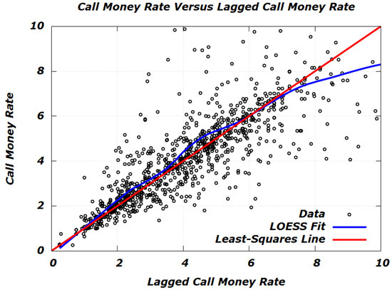
Figure 7. Scatterplot of the monthly broker call rate versus its lagged values. The least-squares line is ${\widehat{y}}_{t+1}=1.587+0.597\times y_t$. LOESS (locally estimated scatterplot smoothing) $\mathrm{bandwidth}:=0.5$.

This means that for every 100 basis points of deviation from its long-run average of $3.94\%$, the broker call rate is expected to close the gap at a rate of 40 basis points per month. However, this mean-reverting behavior is corrupted by random disturbances whose average (root-mean-squared) magnitude is $2.36\%$ per month.

Solving the first-order difference Equation (11) for $\mathrm{Call}{\mathrm{Rate}}_t$ in terms of $\mathrm{Call}{\mathrm{Rate}}_0$, one gets the expression (cf. with Hamilton 1994)

$$\begin{array}{c}\mathrm{Call}{\mathrm{Rate}}_t=\frac{1}{1-\rho L}\left(\alpha +\sigma {ϵ}_{t-1}\right)\hfill \\ =\mu +{\rho }^t\times \left(\mathrm{Call}{\mathrm{Rate}}_0-\mu \right)+\sigma {\displaystyle \sum _{s=0}^{t-1}}{\rho }^{t-1-s}{ϵ}_s\hfill \\ =\underset{\left(0.08\right)}{3.943}+{\underset{\left(0.022\right)}{0.597}}^t\times \left(\mathrm{Call}{\mathrm{Rate}}_0-\underset{\left(0.08\right)}{3.943}\right)+2.362\times {\displaystyle \sum _{s=0}^{t-1}}{\underset{\left(0.022\right)}{0.597}}^{t-1-s}{ϵ}_s.\hfill \end{array}$$

(22)

Thus, our general forecast for the broker call rate t months hence (normalizing today’s date to 0) is

$$\begin{array}{|c|}\hline \mathbb{E}\left[\mathrm{Call}{\mathrm{Rate}}_t|\mathrm{Call}{\mathrm{Rate}}_0\right]=\underset{\left(0.08\right)}{3.943}+{\underset{\left(0.022\right)}{0.597}}^t\times \left(\mathrm{Call}{\mathrm{Rate}}_0-\underset{\left(0.08\right)}{3.943}\right)\\ \hline\end{array}.$$

(23)

The corresponding root-mean-squared forecast error is

$$\begin{array}{c}\mathrm{Std}\left(\mathrm{Call}{\mathrm{Rate}}_t|\mathrm{Call}{\mathrm{Rate}}_0\right)=\frac{\sigma }{\sqrt{1-{\rho }^2}}\sqrt{1-{\rho }^{2t}}=s\sqrt{1-{\rho }^{2t}}\hfill \\ =2.944\times \sqrt{1-{0.356}^t}.\hfill \end{array}$$

(24)

Figure 8 plots the root-mean-squared forecast error against time for $t\in \{0,\dots ,6\}$.

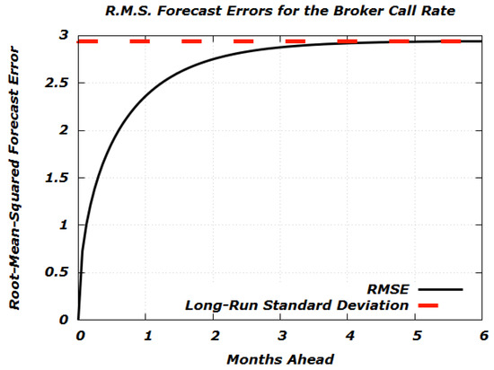
Figure 8. Root-mean-squared forecast errors (in percent) for up to six months ahead.

Example 1 (Out-of-Sample Predictions).

As of this writing2, Bankrate.com reports the following information about the U.S. call money rate:

■

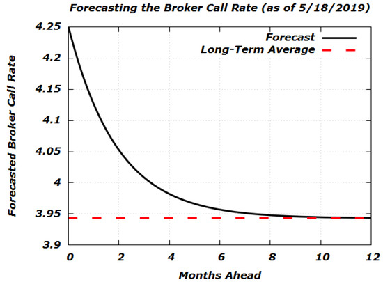
One year ago, the broker call rate was $y_0:=3.5\%$, ($y_0-\mu =-0.443$).

■

One month ago, the broker call rate was $y_{11}=4.25\%$, ($y_{11}-\mu =0.307).$

■

The current U.S. call money rate (as of this writing) is also $y_{12}=4.25\%$.

Thus, from the standpoint of a month ago, today’s call money rate would have been forecasted to be $4.13\%$ (cf. with Figure 9), for a prediction error of $0.12\%$. From the standpoint of a year ago, today’s call money rate would have been forecasted to be $3.94\%$, for a prediction error of $0.31\%$. These errors compare favorably with the root-mean-squared errors plotted in Figure 8.

Figure 9. 12-month forecast for the broker call rate (starting from $y_0:=4.25\%$ on 18 May 2019).

2.3. AR(2) Model

Taking our cue from the fact that Bankrate.com only reports the two most recent monthly observations of the broker call rate, we proceed to estimate a (stationary) second-order autoregressive model for the sake of lowering our root-mean-squared prediction error. Thus, we have the empirical specification

$$y_{t+1}=c+{\varphi }_1{y}_t+{\varphi }_2{y}_{t-1}+\sigma {ϵ}_t,$$

(25)

or, equivalently,

$$\left(1-{\varphi }_{1}L-{\varphi }_2{L}^2\right)y_{t+1}=c+\sigma {ϵ}_t.$$

(26)

The long-run mean is

$$\mu :=\mathbb{E}\left[y_t\right]=\frac{c}{1-{\varphi }_1-{\varphi }_2},$$

(27)

and the unconditional variance (cf. with Fuller 1976) is

$$v:=\mathrm{Var}\left[y_t\right]=\frac{\left(1-{\varphi }_2\right){\sigma }^2}{\left(1+{\varphi }_2\right)\left[{\left(1-{\varphi }_2\right)}^2-{\varphi }_1^2\right]}.$$

(28)

When expressed in mean-deviation form, our empirical specification amounts to

$$y_{t+1}-\mu ={\varphi }_1(y_t-\mu )+{\varphi }_2(y_{t-1}-\mu )+\sigma {ϵ}_t,$$

(29)

or equivalently,

$$\Delta y_t:=y_{t+1}-y_t=-(1-{\varphi }_1)(y_t-\mu )+{\varphi }_2(y_{t-1}-\mu )+\sigma {ϵ}_t.$$

(30)

Table 3 summarizes the results of the autoregression. Our estimated relationship is

$$\begin{array}{|c|}\hline \mathrm{Call}{\mathrm{Rate}}_{t+1}=\underset{\left(0.112\right)}{1.215}+\underset{\left(0.026\right)}{0.456}·\mathrm{Call}{\mathrm{Rate}}_t+\underset{\left(0.026\right)}{0.235}·\mathrm{Call}{\mathrm{Rate}}_{t-1}+2.297{ϵ}_t\\ \hline\end{array}.$$

(31)

Table 3. Parameter estimates for AR(2) model of the U.S. broker call money rate. *** p-value $<0.01.$

Parameter/Regression Statistic	Est./Value	95% Interval
c (Intercept)	1.215 *** (0.112)	[0.995,1.434]
${\varphi }_1$ (Weight on first lagged value)	0.456 *** (0.026)	[0.405,0.508]
${\varphi }_2$ (Weight on second lagged value)	0.235 *** (0.026)	[0.184,0.287]
$\mu =c÷\left(1-{\varphi }_1-{\varphi }_2\right)$ (Long-run mean)	3.938
$\sigma$ (Root-mean-squared prediction error)	2.297
s (Long-run standard deviation)	2.945
Mean absolute residual	1.046
5th percentile absolute residual	0.0778
50th percentile (median) absolute residual	0.716
95th percentile absolute residual	2.884
Roots of lag polynomial $1-{\varphi }_{1}L-{\varphi }_2{L}^2$	{1.309, −3.248}
Characteristic roots (of ${\lambda }^2-{\varphi }_1\lambda -{\varphi }_2)$	{0.764, −0.308}

OLS Estimates for the AR(2) Specification $(R^2=39\%;\mathtt{standard\; errors\; in\; parentheses}).$

For the sake of calculating the general forecast $\mathbb{E}\left[y_t|y_0,y_1\right]$, we must solve the following (deterministic) difference equation (cf. with Spiegel 1971):

$$y_{t+1}=c+{\varphi }_1{y}_t+{\varphi }_2{y}_{t-2}.$$

(32)

A particular solution is of course given by $y_t^p:\equiv \mu$. In order to solve the associated homogeneous equation

$$y_{t+1}={\varphi }_1{y}_t+{\varphi }_2{y}_{t-2},$$

(33)

we will require the roots of the characteristic equation

$${\lambda }^2-{\varphi }_1\lambda -{\varphi }_2=0,$$

(34)

which are

$${\lambda }_{1,2}=\frac{{\varphi }_1\pm \sqrt{{\varphi }_1^2+4{\varphi }_2}}{2}=0.764,-0.308.$$

(35)

Thus, the general solution of the difference Equation (32) is

$$\begin{array}{c}\mathbb{E}\left[y_t|y_0,y_1\right]=\mu +\frac{1}{{\lambda }_2-{\lambda }_1}\left\{\left[{\lambda }_2\left(y_0-\mu \right)-\left(y_1-\mu \right)\right]{\lambda }_1^t+\left[y_1-\mu -{\lambda }_1\left(y_0-\mu \right)\right]{\lambda }_2^t\right\}\hfill \\ =3.938-0.933\times \{\left[-0.308\left(y_0-3.938\right)-\left(y_1-3.938\right)\right]{0.764}^t\hfill \\ +\left[y_1-3.938-0.764\left(y_0-3.938\right)\right]{\left(-0.308\right)}^t\}.\hfill \end{array}$$

(36)

Figure 10 compares the 12-month forecasts of our estimated AR(1) and AR(2) models, given the two most recent observations $y_0:=4.25$ and $y_1:=4.25$. Note that the AR(2) forecast exhibits a significantly slower rate of mean-reversion than its AR(1) counterpart. On that score, Figure 11 plots the two models’ responses to an exogenous 100 basis point impulse in the broker call rate. After six months, the persistent effect on the broker call rate amounts to 14 basis points under the AR(2) model; at the 12-month mark, the marginal effect dissipates to just three basis points.

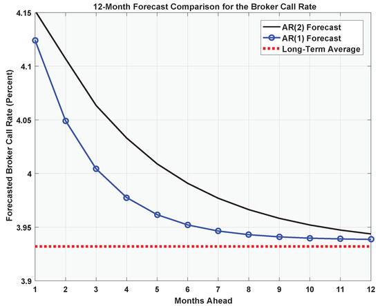
Figure 10. 12-month forecast comparison for AR(1) and AR(2) models of the broker call rate, given the two most recent observations $y_0:=4.25$ and $y_1:=4.25$ (as of 18 May 2019).

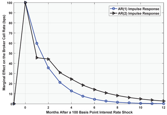
Figure 11. Comparison of model responses to an exogenous 100 basis point impulse in the broker call rate.

2.4. Vasicek Model

To better understand the short-term (intra-month) fluctuations of the broker call rate, we use our monthly AR(1) parameter estimates to help fit an Ornstein–Uhlenbeck model of interest rate evolution in continuous time (cf. with Mikosch 1998). Vasicek (1977) was the first researcher who used the Ornstein–Uhlenbeck processes to model the mean-reverting behavior of interest rates. In our context, we have the following stochastic differential equation (the time t being measured in months):

$$\begin{array}{|c|}\hline d\left(\mathrm{Call}{\mathrm{Rate}}_t\right)=-\overline{\theta }\times \left(\mathrm{Call}{\mathrm{Rate}}_t-\overline{\mu }\right)dt+\overline{\sigma }d{W}_t.\\ \hline\end{array}$$

(37)

Equivalently, we have the integrated form (cf. with Mikosch 1998)

$$\mathrm{Call}{\mathrm{Rate}}_t=\mathrm{Call}{\mathrm{Rate}}_0-\overline{\theta }{\int }_0^t\left(\mathrm{Call}{\mathrm{Rate}}_s-\overline{\mu }\right)ds+\overline{\sigma }{W}_t,$$

(38)

where $W_t$ is a standard Brownian motion and $d{W}_t:=ϵ\times \sqrt{dt}$ is its instantaneous change in position over the differential time step $\left[t,t+dt\right]$. The parameter $\overline{\mu }:=\mathbb{E}\left[\mathrm{Call}{\mathrm{Rate}}_t\right]$ represents the stationary mean, or long-run equilibrium level, of the broker call money rate. The parameter

$$-\overline{\theta }:=\frac{\mathbb{E}\left[d\left(\mathrm{Call}{\mathrm{Rate}}_t\right)|\mathrm{Call}{\mathrm{Rate}}_t\right]}{\mathrm{Call}{\mathrm{Rate}}_t-\overline{\mu }}/dt$$

(39)

denotes the instantaneous rate of mean-reversion, e.g., the expected rate of change in the interest rate as a percentage of its current deviation from the long-run average. Finally, the parameter

$${\overline{\sigma }}^2:=\frac{\mathrm{Var}\left[d\left(\mathrm{Call}{\mathrm{Rate}}_t\right)|\mathrm{Call}{\mathrm{Rate}}_t\right]}{dt}$$

(40)

represents the local variance of interest rate changes per unit time.

The solution of the Ornstein–Uhlenbeck equation (cf. with Mikosch 1998) is

$$\mathrm{Call}{\mathrm{Rate}}_t=\overline{\mu }+exp\left(-\overline{\theta }t\right)\times \left(\mathrm{Call}{\mathrm{Rate}}_0-\overline{\mu }\right)+\overline{\sigma }{\int }_0^{t}exp\left(-\overline{\theta }(t-s)\right)d{W}_s,$$

(41)

and the stationary (long-term) standard deviation is

$$\mathrm{Std}\left(\mathrm{Call}{\mathrm{Rate}}_t\right)=\frac{\overline{\sigma }}{\sqrt{2\overline{\theta }}}.$$

(42)

The corresponding t-month ahead forecast is

$$\mathbb{E}\left[\mathrm{Call}{\mathrm{Rate}}_t|\mathrm{Call}{\mathrm{Rate}}_0\right]=\overline{\mu }+exp\left(-\overline{\theta }t\right)\times \left(\mathrm{Call}{\mathrm{Rate}}_0-\overline{\mu }\right),$$

(43)

and the root-mean-squared forecast error is

$$\mathrm{Std}\left(\mathrm{Call}{\mathrm{Rate}}_t|\mathrm{Call}{\mathrm{Rate}}_0\right)=\frac{\overline{\sigma }}{\sqrt{2\overline{\theta }}}\times \sqrt{1-exp\left(-2\overline{\theta }t\right)}.$$

(44)

In order to reconcile the conditional forecast function (43) with the AR(1) forecast $\mathbb{E}\left[\mathrm{Call}{\mathrm{Rate}}_t|\mathrm{Call}{\mathrm{Rate}}_0\right]=\mu +{\rho }^t\times \left(\mathrm{Call}{\mathrm{Rate}}_0-\mu \right)$, we must have

$$\overline{\mu }:=\mu =3.943\mathrm{and}$$

(45)

$$\overline{\theta }:=-log\rho =0.516.$$

(46)

In order to reconcile the long-run standard deviation (42) with its AR(1) counterpart $s=\sigma ÷\sqrt{1-{\rho }^2}$, we must have

$$\overline{\sigma }:=s\sqrt{-2log\rho }=\sigma \sqrt{\frac{-2log\rho }{1-{\rho }^2}}=2.99.$$

(47)

Thus, the following three equations summarize our estimated law of (continuous) motion for the U.S. broker call rate.

Differential Form:

$$\begin{array}{|c|}\hline d\left(\mathrm{Call}{\mathrm{Rate}}_t\right)=-0.516\times \left(\mathrm{Call}{\mathrm{Rate}}_t-3.943\right)dt+2.99\times d{W}_t,\\ \hline\end{array}$$

(48)

Integral Form:

$$\begin{array}{|c|}\hline \mathrm{Call}{\mathrm{Rate}}_t=\mathrm{Call}{\mathrm{Rate}}_0-0.516{\int }_0^t\left(\mathrm{Call}{\mathrm{Rate}}_s-3.943\right)ds+2.99\times W_t,\\ \hline\end{array}$$

(49)

Explicit Form:

$$\begin{array}{|c|}\hline \mathrm{Call}{\mathrm{Rate}}_t=3.943+{0.597}^t\times \left(\mathrm{Call}{\mathrm{Rate}}_0-3.943\right)+2.99\times {\int }_0^t{0.597}^{t-s}d{W}_s.\\ \hline\end{array}$$

(50)

Figure 12 plots the result of an intra-month simulation of the U.S. broker call rate, starting from an initial level of $y_0:=4.25$.

Figure 12. Intra-month simulation of the (continuously-compounded) U.S. broker call rate ($y_0:=4.25$).

3. Implications for Margin Loan Pricing

For the sake of this section, so as to avoid any confusion, all interest rates, standard deviations, drifts, etc. will now be reported as numbers belonging to the unit interval $\left[0,1\right]$ (rather than as percentages between 0 and 100).

In the author’s prior work on margin loan pricing in continuous time (Garivaltis 2019a, 2019b), he derived the simple theoretical relationship

$$\mathrm{Margin}\mathrm{Loan}\mathrm{Interest}{\mathrm{Rate}}_t=\frac{\mathrm{Broker}\mathrm{Call}{\mathrm{Rate}}_t}{2}+C,$$

(51)

where C is a constant that is independent of the broker call rate and independent of the time t. This was done by assuming that the broker’s sole (representative) client is a continuous time Kelly gambler (cf. with Luenberger 1998) who borrows cash over each differential time step $\left[t,t+dt\right]$ for the sake of leveraged betting on a single risk asset (say, the market index) whose price $S_t$ follows the geometric Brownian motion

$$d{S}_t:=S_t\times \left({\mu }_{S}dt+{\sigma }_{S}d{W}_t^S\right),$$

(52)

$$d\left(log{S}_t\right)=\left({\mu }_S-\frac{{\sigma }_S^2}{2}\right)dt+{\sigma }_{S}d{W}_t^S.$$

(53)

Here, we have used the symbol $d{W}^S\left(t\right)$ to denote the standard Brownian motion that drives the asset price; the drift and volatility are ${\mu }_S$ and ${\sigma }_S$, respectively. The corresponding Kelly bet (cf. with Thorp 2006) for this market over the interval $[t,t+dt]$ amounts to the client betting the fraction

$$b\left(r_L\right):=\frac{{\mu }_S-r_L}{{\sigma }_S^2}$$

(54)

of his wealth on the stock, where $r_L$ denotes the continuously-compounded interest rate charged by the broker for the duration $\left[t,t+dt\right]$. Thus, the instantaneous quantity of margin loans demanded per dollar of client equity (e.g., the instantaneous demand curve) is given by the formula

$$q\left(r_L\right):=b\left(r_L\right)-1=\left(\frac{{\mu }_S}{{\sigma }_S^2}-1\right)-\frac{1}{{\sigma }_S^2}\times r_L.$$

(55)

Equivalently, the broker faces the inverse (instantaneous) demand curve

$$r_L=\left({\mu }_S-{\sigma }_S^2\right)-{\sigma }_S^2\times q$$

(56)

for the duration $\left[t,t+dt\right]$. On account of the fact that the broker has constant marginal cost (viz. the broker call rate), the corresponding monopoly midpoint price is

$$\begin{array}{c}\mathrm{Margin}{\mathrm{Rate}}_t=\frac{\mathrm{Marginal}{\mathrm{Cost}}_t+\mathrm{Choke}\mathrm{Price}}{2}\hfill \\ =\frac{\mathrm{Call}{\mathrm{Rate}}_t}{2}+\frac{{\mu }_S-{\sigma }_S^2}{2}=\frac{\mathrm{Call}{\mathrm{Rate}}_t}{2}+\frac{1}{2}\left({\nu }_S-\frac{{\sigma }_S^2}{2}\right),\hfill \end{array}$$

(57)

where the parameter ${\nu }_S:={\mu }_S-{\sigma }_S^2/2$ represents the expected compound (logarithmic) growth rate of the market index (say, the S&P 500). Thus, our constant C is given by

$$C:=\frac{{\nu }_S}{2}-\frac{{\sigma }_S^2}{4}.$$

(58)

Given the backdrop of our mean-reverting empirical model of the broker call rate, the theoretical pricing formula (51) implies that the margin loan interest rates charged by brokers must also follow an Ornstein–Uhlenbeck process. For, we have

$$d\left(\mathrm{Margin}{\mathrm{Rate}}_t\right)=\frac{d\left(\mathrm{Call}{\mathrm{Rate}}_t\right)}{2}=-\frac{\overline{\theta }}{2}\left(\mathrm{Call}{\mathrm{Rate}}_t-\overline{\mu }\right)dt+\frac{\overline{\sigma }}{2}d{W}_t.$$

(59)

Bearing in mind that $\mathrm{Call}{\mathrm{Rate}}_t=2\times \left(\mathrm{Margin}{\mathrm{Rate}}_t-C\right)$, we get the law of motion

$$\begin{array}{|c|}\hline d\left(\mathrm{Margin}{\mathrm{Rate}}_t\right)=-\overline{\theta }\times \left(\mathrm{Margin}{\mathrm{Rate}}_t-\frac{\overline{\mu }}{2}-C\right)dt+\frac{\overline{\sigma }}{2}d{W}_t.\\ \hline\end{array}$$

(60)

Thus, we conclude that the long-run average of the margin loan interest rate charged by stock brokers should be $\overline{\mu }/2+C$, and that margin loan prices should exhibit the same level of mean reversion ($\overline{\theta }$) as the broker’s cost of funding. However, the random fluctuations in the margin loan interest rate should have half the magnitude of the corresponding movements in the broker call rate.

Following Garivaltis (2019b), if we use the stylized parameters ${\nu }_S:=0.09,{\sigma }_S:=0.15,\mathrm{and}{\mu }_S:={\nu }_S+{\sigma }_S^2/2$ to represent the (annual) dynamics of the S&P 500 index, then we get $C=0.03938$. Thus, our hybrid empirical/theoretical model of the margin loan interest rate is

$$\begin{array}{|c|}\hline d\left(\mathrm{Margin}{\mathrm{Rate}}_t\right)=-0.516\times \left(\mathrm{Margin}{\mathrm{Rate}}_t-0.05909\right)+0.01495\times d{W}_t.\\ \hline\end{array}$$

(61)

On account of the linear relationship $b=\left({\mu }_S-r_L\right)÷{\sigma }_S^2$ between the margin loan interest rate and the bet size b, it follows that the client’s quantity $q=b-1$ of margin loans per dollar of equity must also follow an Ornstein-Uhlenbeck process. A straightforward calculation shows that

$$\begin{array}{|c|}\hline d{b}_t=d{q}_t=-\overline{\theta }\times \left(q_t-\frac{{\mu }_S-\overline{\mu }}{2{\sigma }_S^2}\right)dt-\frac{\overline{\sigma }}{2{\sigma }_S^2}d{W}_t,\\ \hline\end{array}$$

(62)

where the time t is measured in months and $W_t$ is the standard Brownian motion that drives the broker call rate. Thus, the leverage ratio of the (representative) Kelly gambler reverts to its long-term mean of $\left({\mu }_S-\overline{\mu }\right)÷\left(2{\sigma }_S^2\right)$ at the same rate $\overline{\theta }$ as the broker call rate and the margin loan interest rate. Given our empirical findings, we have the concrete (monthly) law of motion:

$$\begin{array}{|c|}\hline d{b}_t=-0.516\times \left(b_t-2.0338\right)dt-0.6644\times d{W}_t.\\ \hline\end{array}$$

(63)

Thus, the long-term average leverage ratio of continuous time Kelly gamblers is $\overline{b}:=2.0338$, for an average quantity of $\overline{q}:=\$1.0338$ borrowed per dollar of client equity. The (stationary) standard deviation of the clients’ leverage ratios is

$$\begin{array}{|c|}\hline \mathrm{Std}\left(b_t\right)=\frac{\overline{\sigma }}{2{\sigma }_S^2\sqrt{2\overline{\theta }}}\\ \hline\end{array}=0.654.$$

(64)

Figure 13 plots a 12-month simulation of the leverage ratios of Kelly gamblers, assuming an initial value of $b_0:=2$.

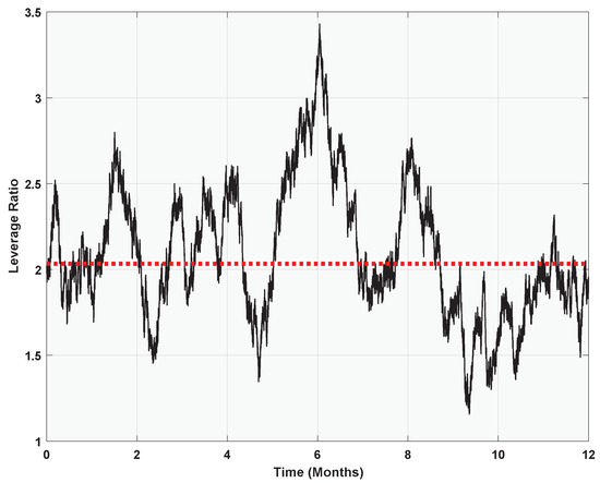
Figure 13. The 12-month simulation of Kelly gamblers’ leverage ratios ($b_0:=2$).

“A fuller account would address the pledging of customers’ securities by broker-dealers to obtain loans from financial institutions.”

—Fortune (2000), in the New England Economic Review.

4. Arbitrage Pricing of Call Loans

In this section, we use Merton’s (1974, 1992) no-arbitrage approach to corporate liability pricing to derive theoretical formulas for the broker call rate and the net interest margin that banks should earn on such loans. On that score, we let r denote the risk-free rate of interest, and we let $\underline{R}$ denote the broker call rate, where $\rho :=\underline{R}-r>0$ is the corresponding risk premium. The broker himself charges his retail customers a margin loan interest rate of $\overline{R}>\underline{R}$. We assume that the (representative) brokerage client borrows D dollars to finance the purchase of a single share of a risky stock or index, whose initial price at time 0 is $S_0$. The client’s initial equity is $E_0:=S_0-D>0$. As usual, we assume that the asset price follows the geometric Brownian motion

$$d{S}_t:=S_t\times \left(\mu dt+\sigma d{W}_t\right),$$

(65)

where $\mu$ is the annual drift rate, $\sigma$ is the annual volatility, and $W_t$ is a standard Brownian motion3. Interest is assumed to compound continuously over the loan term $[0,T]$, so that the client’s accumulated margin loan (debit) balance at time t is $D{e}^{\overline{R}t}$. Thus, his equity fluctuates according to the random process $E_t:=S_t-D{e}^{\overline{R}t}$.

If the broker was willing or able to continuously monitor the client’s account for solvency, then there would be no credit risk, for, on account of the continuous sample path of ${\left(E_t\right)}_{t\in \left[0,T\right]}$, the broker could liquidate the account the instant that $E_t=0$ (or some other threshold $\underline{E}$). Thus, under continuous monitoring, there is certainly no risk to the bank that funded part of the margin loan; in this case, the no-arbitrage axiom dictates that $\underline{R}=r$. In order to have $\underline{R}>r$ in equilibrium, we must start with a situation whereby it is possible for the retail client to default on his margin loan. Thus, as in Fortune (2000) and Garivaltis (2019a), we assume that the broker does not monitor the client’s account for solvency until some given maturity date, T.

However, if the broker is willing to maintain a dynamically precise short position in the risk asset (cf. with Fortune 2000 and Garivaltis 2019a), then it is possible, in the sense of Black and Scholes (1973), to completely “eliminate risk” through continuous trading in the underlying. In this happenstance, the no-arbitrage principle implies a unique margin loan interest rate $\overline{R}>r$, but it fails to give us a characterization of the call money rate, since there is no actual risk to the bank that funded the margin loan. Thus, in order to generate risk premia in the call money market, we must make the twin assumptions:

■

The broker does not check the client’s portfolio for solvency until the maturity date, T.

■

The broker is not willing or able to hedge his own default risk.

In this environment, we now have the possibility of a “default cascade” whereby the client defaults on his margin loan at T, and this in turn causes the broker to default on his debt to the money market. Accordingly, we will assume that the broker borrows $d<D$ dollars on the money market for the sake of funding the D dollar margin loan; the remaining $D-d$ dollars of the margin loan constitute the broker’s own equity. That is, we have the decomposition

$$\begin{array}{c}\mathrm{Total}\mathrm{Leveraged}\mathrm{Portfolio}\mathrm{Value}=\mathrm{Client}’\mathrm{s}\mathrm{Equity}\hfill \\ +\mathrm{Broker}’\mathrm{s}\mathrm{Equity}+\mathrm{Call}\mathrm{Loan}\mathrm{Balance}.\hfill \end{array}$$

(66)

Equivalently, this means that for $0\le t<T$, we have

$$\begin{array}{c}\mathrm{Broker}’\mathrm{s}{\mathrm{Equity}}_t=S_t-E_t-d{e}^{\underline{R}t}=D{e}^{\overline{R}t}-d{e}^{\underline{R}t}\hfill \\ =\mathrm{Broker}’\mathrm{s}{\mathrm{Assets}}_t-\mathrm{Broker}’\mathrm{s}{\mathrm{Liabilities}}_t.\hfill \end{array}$$

(67)

Following Fortune (2000) and Garivaltis (2019a), we assume that the retail client will abandon his account at T if $E_T\le 0$, leaving the broker with collateral worth $S_T$. Thus, the broker’s assets at the end of the loan term amount to

$$min\left(S_T,D{e}^{\overline{R}T}\right),$$

(68)

and the broker’s final equity is equal to

$$min\left(S_T,D{e}^{\overline{R}T}\right)-d{e}^{\underline{R}t}.$$

(69)

If the broker’s final equity is $\le 0$, then he himself will default on his debt to the money market, leaving his creditors with collateral in the amount of $min\left(S_T,D{e}^{\overline{R}T}\right)$. Thus, the final payoff that accrues at T to the bank that made the call loan is

$$min\left\{min\left(S_T,D{e}^{\overline{R}T}\right),d{e}^{\underline{R}t}\right\}=min\left(S_T,d{e}^{\underline{R}t}\right),$$

(70)

where we have made use of the fact that $d<D$ and $\underline{R}<\overline{R}$. Table 4 summarizes the three possible credit events faced by the call lender.

Table 4. The three possible credit events faced by the call lender.

Credit Event	Upshot
$S_T\ge D{e}^{\overline{R}T}$	No defaults.
$d{e}^{\underline{R}T}\le S_T<D{e}^{\overline{R}T}$	Retail client defaults but broker does not.
$S_T<d{e}^{\underline{R}T}$	Retail client and broker both default.

The propagation of margin loan risk in Black–Scholes markets.

Assuming that the bank’s call money was itself borrowed at the risk-free rate r, the bank’s final profit (loss) is

$${\pi }_T:=min\left(S_T,d{e}^{\underline{R}T}\right)-d{e}^{rT}.$$

(71)

Making use of the fact that $min\left(x,y\right)=x+y-max\left(x,y\right)$, we have

$$\begin{array}{c}{\pi }_T=S_T+d{e}^{\underline{R}T}-max\left(S_T,d{e}^{\underline{R}T}\right)-d{e}^{rT}\hfill \\ =S_T-d{e}^{rT}-\left[max\left(S_T,d{e}^{\underline{R}T}\right)-d{e}^{\underline{R}T}\right]\hfill \\ =\begin{array}{|c|}\hline S_T-d{e}^{rT}-max\left(S_T-K,0\right),\\ \hline\end{array}\hfill \end{array}$$

(72)

where $K:=d{e}^{\underline{R}T}$. That is to say, the bank’s (random) profit ${\pi }_T$ amounts to the final payoff of the following portfolio:

■

Long one share of the stock

■

Short d dollars at the risk-free rate of interest

■

Short one European-style call option at a strike price of $K:=d{e}^{\underline{R}T}$.

Naturally, the bank can hedge its (net long) exposure to the underlying (e.g., the bank has de facto written a covered call) by shorting a dynamically precise amount of the retail client’s portfolio. In order to prevent riskless arbitrage opportunities, the time-0 expected present value of the bank’s profit with respect to the equivalent martingale measure ($\mathbb{Q}$) must be zero:

$$e^{-rT}{\mathbb{E}}_0^{\mathbb{Q}}\left[{\pi }_T\right]=S_0-d-\mathrm{BSCall}\left(S_0,0,K,r,\sigma ,T\right)=0.$$

(73)

Recalling the Black and Scholes (1973) formula

$$\mathrm{BSCall}\left(S_0,0,K,r,\sigma ,T\right)=S_{0}N\left(d_1\right)-K{e}^{-rT}N\left(d_2\right),$$

(74)

where

$$d_1:=\frac{log\left(S_0/K\right)+\left(r+{\sigma }^2/2\right)T}{\sigma \sqrt{T}}$$

(75)

and

$$d_2:=d_1-\sigma \sqrt{T},$$

(76)

and simplifying, we get the following equation characterizing the broker call rate:

$$\begin{array}{|c|}\hline \frac{d}{S_0}=\frac{N(-d_1)}{1-N\left(d_2\right)\times exp\left(\rho T\right)},\\ \hline\end{array}$$

(77)

where $\rho :=\underline{R}-r$ is the risk premium for call money,

$$-d_1=\frac{log\left(d/S_0\right)+\left(\rho -{\sigma }^2/2\right)T}{\sigma \sqrt{T}},$$

(78)

and the ratio $d÷S_0$ represents the percentage of the portfolio that has been financed by call money. As usual, $N(•)$ denotes the cumulative normal distribution function.

Note that the broker call rate $\underline{R}$ does not depend on the drift $\mu$ or on the margin loan interest rate $\overline{R}$ that the broker charges its clients. The characterization (77) of $\underline{R}$ is not particular to the numerical levels of d and $S_0$; it only depends on their ratio $d÷S_0$. Similarly, the numbers r and $\underline{R}$ only matter to (77) in so far as their difference $\rho :=\underline{R}-r$ is featured prominently. That is to say (cf. with Merton 1974, 1992), the risk premium for call money depends only on the following credit characteristics:

■

T (the loan term);

■

$d÷S_0$ (the loan-to-value ratio);

■

$\sigma$ (the volatility of the collateral).

The bank’s net exposure to the underlying in state $(S_t,t)$ is equal to (cf. with Wilmott 1998):

$$\Delta (S,t):=\frac{\partial }{\partial S}\left[S-d{e}^{rt}-\mathrm{BSCall}\left(S,t,K,r,\sigma ,T\right)\right]=1-N\left(d_1\right)=N(-d_1).$$

(79)

Thus, $\Delta =N(-d_1)$ represents the (dynamic) percentage of the retail client’s portfolio that must be sold short by banks in order to hedge their counterparty risk.

Figure 14 plots the implied loan-to-value ratio $d÷S_0$ and the implied short position $\Delta =N(-d_1)$ for different values $\underline{R}$ of the broker call rate. Here, we have assumed a risk-free rate of $r:=2.088\%$ (which is the current 5-year U.S. Treasury yield as of this writing), a 90-day loan term ($T:=90÷365$), and a conservative value of $\sigma :=40\%$ annual stock market volatility.

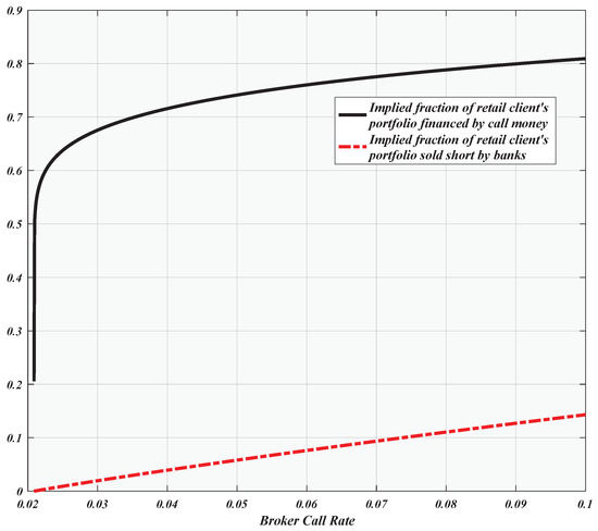
Figure 14. The implied loan-to-value ratios ($d÷S_0$) and hedge ratios ($\Delta )$ for different values of the broker call rate ($r:=2.088\%,T:=90÷365,\sigma :=40\%$).

Thus, we have obtained the following (“puzzling”) conclusion: even under the conservative assumptions of a long (90-day) loan term and very high ($40\%$) annual stock market volatility, the no-arbitrage axiom implies that $72.3\%$ (!!) of the value of all U.S. leveraged portfolios has been financed by call money. This means that the sum total of broker and client equity must amount to only $27.7\%$ of the value of all leveraged portfolios. These figures contradict the well-known legal constraint (e.g., U.S. Regulation-T) on retail margin debt:

$$d÷S_0\le \underset{\mathrm{U}.\mathrm{S}.\text{Regulation-T}.}{\underbrace{D÷S_0\le 0.5}}.$$

(80)

To avoid this logical contradiction, we must admit the possibility that the banks and financial institutions that lend call money to stock brokers in the United States may be earning substantial arbitrage profits on the spread over the risk-free rate.

Note well that varying the term of the call loan is of no great help in resolving the puzzle; indeed, Figure 15 plots the implied maturities T that would rationalize different values $\underline{R}$ of the broker call rate, assuming the parameters $r:=2.088\%,\sigma :=40\%$4, and $d÷S_0:=50\%.$ For the currently observed call rate of $4.25\%$, we get an implied loan term of $1.75$ years and an implied delta in the amount of $6.6\%$ of the retail client’s portfolio.

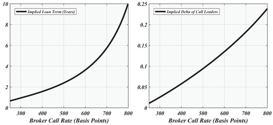
Figure 15. The implied loan terms (T) and hedge ratios ($\Delta$) for different values of the broker call rate ($r:=2.088\%,\sigma :=40\%,d÷S_0:=50\%$).

5. Summary and Conclusions

This paper contributed to the empirical literature on margin loans in the stock markets of developed economies by taking a novel approach to some financial time series (specifically, brokers’ margin loan interest rates and the leverage ratios of their most sophisticated clients) that have been historically difficult to observe by the econometrician. Specifically, we derived hybrid empirical/theoretical models of these stochastic processes by combining empirical data on the U.S. broker call money rate (e.g., stock brokers’ overnight cost of funding) with the author’s prior theoretical formulas on pricing margin loans to Kelly gamblers (Garivaltis 2019a, 2019b).

Thus, we described and analyzed a collection of 1367 monthly observations of the U.S. broker call rate (1857:01 through 1970:11) supplied by the Federal Reserve Bank of St. Louis (FRED). Our estimated AR(1) specification (and corresponding Ornstein–Uhlenbeck model) indicates that for every 100 basis points of deviation from its long-term average of $3.943\%$, the (continuously-compounded) broker call rate will revert to the mean at an expected rate of $40.3$ basis points per month, but this reversion is disturbed by monthly innovations whose root-mean-squared magnitude is $2.362\%$. Buoyed by the fact that Bankrate.com reports the two most recent observations of the broker call money rate (4.25% as of this writing), we constructed an AR(2) model that reduced the monthly root-mean-squared prediction error (in-sample) by 6.5 basis points, to $2.297\%$.

We proceeded to reconcile this empirical law of motion with following theoretical relationship (Garivaltis 2019a), based on instantaneous monopoly pricing of margin loans to Kelly gamblers:

$$\mathrm{Margin}\mathrm{Loan}\mathrm{Interest}{\mathrm{Rate}}_t=\frac{1}{2}\left(\mathrm{Broker}\mathrm{Call}{\mathrm{Rate}}_t\right)+\frac{1}{2}\left({\nu }_S-\frac{{\sigma }_S^2}{2}\right),$$

(81)

where ${\nu }_S$ denotes the long-run compound annual (logarithmic) growth rate of the stock market, and ${\sigma }_S$ is its annual volatility. Under this arrangement, only half of the random movements in the broker call rate get passed on to retail consumers. Assuming the stylized parameter values ${\nu }_S:=0.09$ and ${\sigma }_S:=0.15$ for the S&P 500 index, we obtained a hybrid empirical/theoretical law of motion for the margin loan interest rate charged by stock brokers:

$$d\left(\mathrm{Margin}{\mathrm{Rate}}_t\right)=-0.516\times \left(\mathrm{Margin}{\mathrm{Rate}}_t-5.909\right)dt+1.495\times d{W}_t.$$

(82)

Thus, the margin loan interest rate will display the same rate of (continuous) mean-reversion as does the broker call rate; the unanticipated instantaneous changes in the margin rate (=$1.495\times d{W}_t$) will be half the size of the corresponding movements in the broker call rate. We then derived a stochastic differential equation that governs the (monthly) leverage ratios ($b_t$) of continuous time Kelly gamblers:

$$d{b}_t=-0.516\times \left(b_t-2.0338\right)dt-0.6644\times d{W}_t.$$

(83)

Hence, our empirical finding is that the long-term average interest rate on margin loans should be $5.9\%$, and that the leverage ratios of sophisticated brokerage clients should oscillate randomly about an equilibrium level of 2.03:1.

Finally, we used Merton’s (1974) no-arbitrage method to uniquely characterize the correct risk premium $\rho :=\underline{R}-r$ that commercial banks should earn on their loans to stock brokers. We assumed that brokers loan money to retail clients at a marked-up rate of $\overline{R}>\underline{R}$; to generate risk premia in the market for call money, we had to assume that stock brokers are not willing or able to short their customers’ portfolios for the sake of hedging the default risk.

Thus, we modeled a situation whereby commercial banks are exposed to the risk of a cascaded default, meaning that the retail client defaults on his margin loan and the brokerage in turn defaults on its debt to the money market. The commercial bank can hedge this risk by shorting the dynamically precise fraction

$$\Delta =N\left(\frac{log(d/S_t)+\left(\rho -{\sigma }^2/2\right)(T-t)}{\sigma \sqrt{T-t}}\right),$$

(84)

of the retail client’s portfolio at time t, where T is the maturity date of the call loan, $\rho$ is the risk premium for call money, $d/S_t$ is the percentage of the client’s portfolio that is financed with call money (as opposed to broker equity and client equity), and $\sigma$ is the annual volatility of the collateral.

Under very conservative assumptions ($40\%$ annual volatility and a 90-day loan term), we concluded that call lenders’ current level of exposure to the stock market amounts to $\Delta =4.4\%$ of the value of all leveraged portfolios in the United States. Comparing the current broker call rate of $4.25\%$ with the prevailing U.S. Treasury yields, we found that the implied loan-to-value ratio is north of $70\%$. This is absurd on account of U.S. Regulation-T, which caps the loan-to-value ratios of retail margin borrowers at $50\%$. In order to alleviate this apparent contradiction, we must live with the possibility that U.S. banks who deal in the market for call money could in fact be earning substantial arbitrage profits on the spread of the broker call rate over the risk-free rate.

References

- Black, Fischer, and Myron Scholes. 1973. The Pricing of Options and Corporate Liabilities. Journal of Political Economy 81: 637–54. [Google Scholar] [CrossRef]
- Fortune, P. 2000. Margin Requirements, Margin Loans, and Margin Rates: Practice and Principles. New England Economic Review, 19–44. [Google Scholar]
- Fortune, P. 2001. Margin Lending and Stock Market Volatility. New England Economic Review, 3–26. [Google Scholar]
- Fuller, W. A. 1976. Introduction to Statistical Time Series. New York: John Wiley & Sons. [Google Scholar]
- Garivaltis, A. 2019a. Two Resolutions of the Margin Loan Pricing Puzzle. Research in Economics 73: 199–207. [Google Scholar] [CrossRef]
- Garivaltis, A. 2019b. Nash Bargaining Over Margin Loans to Kelly Gamblers. Risks 7: 93. [Google Scholar] [CrossRef]
- Hamilton, J. D. 1994. Time Series Analysis. Princeton: Princeton University Press. [Google Scholar]
- Hardouvelis, G. A., and S. Peristiani. 1992. Margin Requirements, Speculative Trading, and Stock Price Fluctuations: The Case of Japan. The Quarterly Journal of Economics 107: 1333–70. [Google Scholar] [CrossRef]
- Hardouvelis, G. A., and P. Theodossiou. 2002. The Asymmetric Relation Between Initial Margin Requirements and Stock Market Volatility Across Bull and Bear Markets. The Review of Financial Studies 15: 1525–59. [Google Scholar] [CrossRef]
- Hirose, T., H. K. Kato, and M. Bremer. 2009. Can Margin Traders Predict Future Stock Returns in Japan? Pacific-Basin Finance Journal 17: 41–57. [Google Scholar] [CrossRef]
- Kelly, J. L. 1956. A New Interpretation of Information Rate. The Bell System Technical Journal, 25–34. [Google Scholar] [CrossRef]
- Lepetit, L., E. Nys, P. Rous, and A. Tarazi. 2008. The Expansion of Services in European Banking: Implications for Loan Pricing and Interest Margins. Journal of Banking & Finance 32: 2325–35. [Google Scholar]
- Luenberger, D. G. 1998. Investment Science. New York: Oxford University Press. [Google Scholar]
- Merton, R. C. 1974. On the Pricing of Corporate Debt: The Risk Structure of Interest Rates. The Journal of Finance 29: 449–70. [Google Scholar]
- Merton, R. C. 1992. Continuous-Time Finance. Cambridge: Basil Blackwell. [Google Scholar]
- Mikosch, T. 1998. Elementary Stochastic Calculus, with Finance in View. River Edge: World Scientific Publishing Company. [Google Scholar]
- Nash, J. 1950. The Bargaining Problem. Econometrica 18: 155–62. [Google Scholar] [CrossRef]
- Sentana, E., and S. Wadhwani. 1992. Feedback Traders and Stock Return Autocorrelations: Evidence from a Century of Daily Data. The Economic Journal 102: 415–25. [Google Scholar] [CrossRef]
- Spiegel, M. R. 1971. Schaum’s Outline of Theory and Problems of Calculus of Finite Differences and Difference Equations. New York: McGraw-Hill Book Company. [Google Scholar]
- Thorp, E. O. 2006. The Kelly Criterion in Blackjack, Sports Betting, and the Stock Market. In Handbook of Asset and Liability Management, Volume 1: Theory and Methodology. Amsterdam: North-Holland Publishing Company. [Google Scholar]
- Vasicek, O. 1977. An Equilibrium Characterization of the Term Structure. Journal of Financial Economics 5: 177–88. [Google Scholar] [CrossRef]
- Watanabe, T. 2002. Margin Requirements, Positive Feedback Trading, and Stock Return Autocorrelations: The Case of Japan. Applied Financial Economics 12: 395–403. [Google Scholar] [CrossRef]
- Wilmott, P. 1998. Derivatives: The Theory and Practice of Financial Engineering. Chichester: John Wiley & Sons. [Google Scholar]