Abstract
Given ongoing financial disintermediation and the need for central banks to establish interest rate corridors, commercial banks have increasingly enriched their asset allocation choices, forming an allocation pattern that combines traditional credit assets (loans) and financial assets (interbank and securities investment). Due to the long-standing dual interest rate system in China, the yields of credit assets and financial assets have differed, which means the latter has greater volatility. Using the quarterly panel data of 23 listed commercial banks in China from 2002 to 2017, the empirical results of this paper show that the fluctuation of the return rate of the two types of assets will affect the asset allocation of banks. Specifically, on the one hand, when the price of financial assets falls, which leads to the narrowing of the credit spread between the two types of assets, banks reduce transaction demand to prevent loss and reduce their holdings of financial assets, thus increasing the ratio of their credit assets to financial assets. On the other hand, rising benchmark lending rates leads to the increase in the credit financing cost of demanders, reducing the willingness of demanders to lend, forcing the demander to obtain funds through other channels. This results in the decrease in the ratio of credit assets to financial assets. Furthermore, the financial characteristics of banks also influence the dynamic adjustment range of asset allocation. That is, the lower the reserve ratio and capital adequacy ratio, the smaller the impact of financial asset yield volatility on bank asset allocation.
Keywords:
financial market shock; credit assets; financial assets; financial characteristics of banks JEL Classification:
G20; G21
1. Introduction
1.1. Background
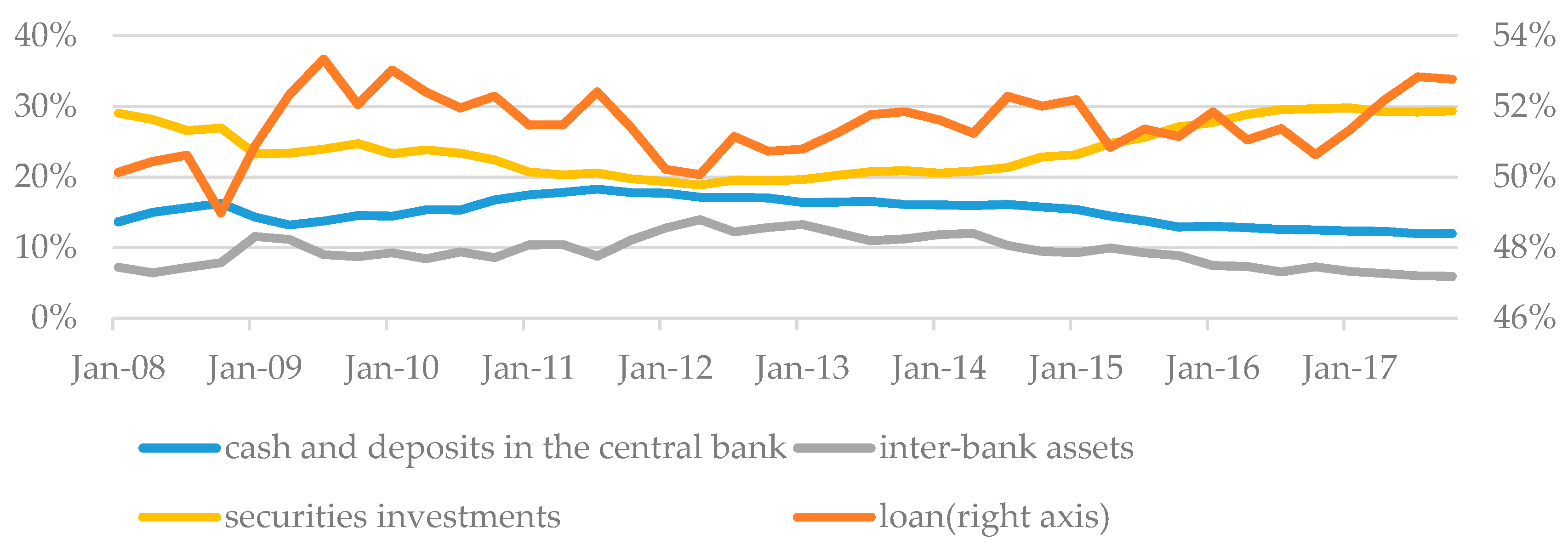
With the development of various financial products and the expansion of financial market participants, the depth and breadth of the market are constantly increasing. China’s financial market runs an indirect financing system dominated by commercial banks. Therefore, the continuous improvement of financial markets profoundly impacts the asset allocation of commercial banks. Figure 1 shows the trend of the proportion of various assets in commercial banks.
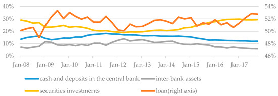
Figure 1.
The trend of assets of commercial banks. (Data sources: Wind).
In 2007, bank loans accounted for 52.4 percent of total bank assets. This proportion declined to 49.4 percent in 2017. The proportion of securities assets and inter-bank assets has been stable at around 25% and 10% respectively. Securities and other financial assets have become the most important asset allocation for commercial banks except loans.
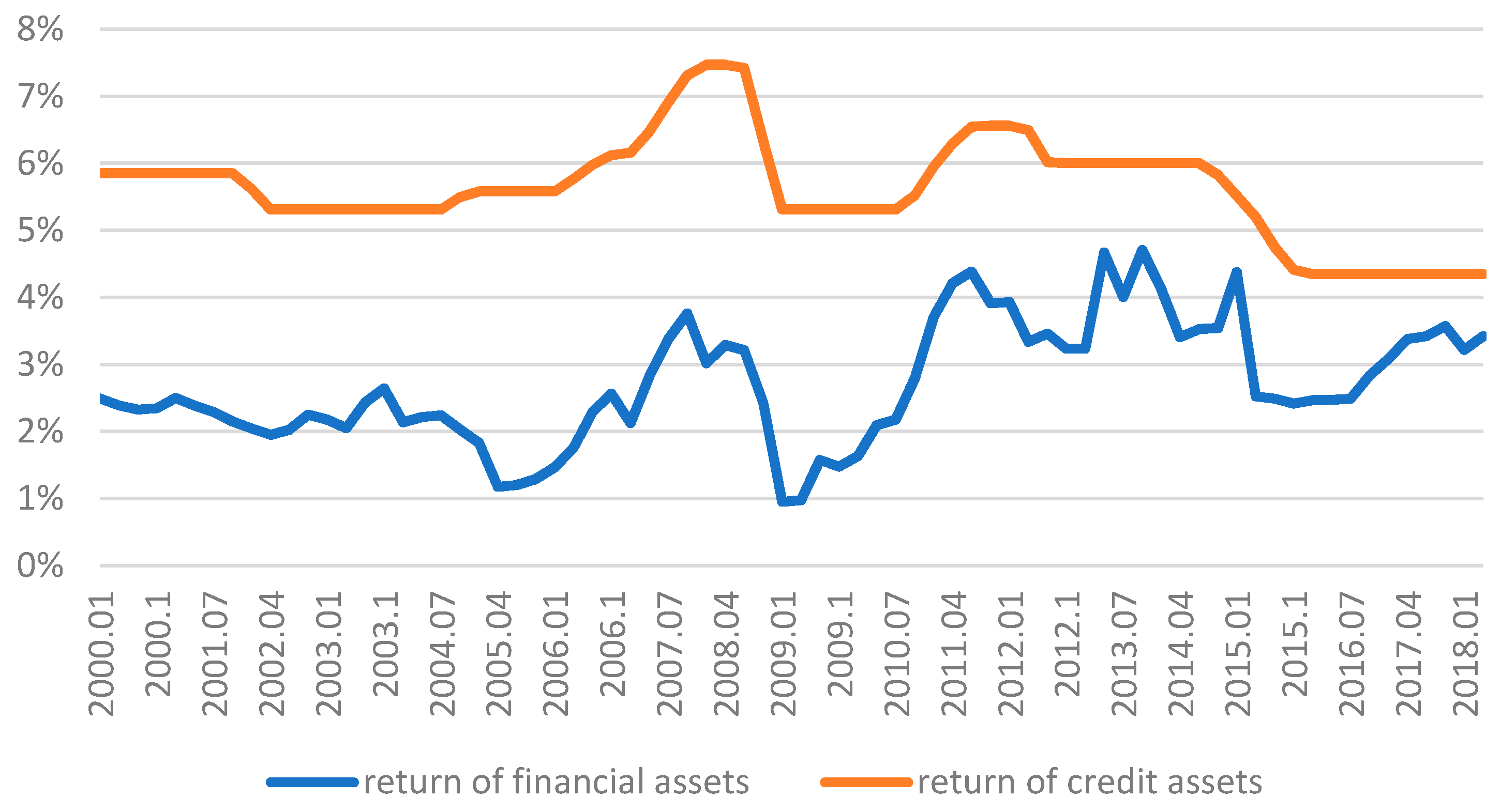
According to the analysis above, this paper classifies bank assets into two categories: traditional credit assets, which are known as loans, and financial assets, which encompass securities investment and inter-bank assets. The classification is based on the volatility of the returns on assets. Before 2013, the loan interest rate was directly controlled by the regulatory authorities. After 2013, although interest rate regulation gradually relaxed, the existence of window guidance and market interest rate pricing self-regulation mechanisms prevented the loan benchmark interest rate from varying flexibly with the market environment, in contrast to the interest rate of financial assets. However, the financial assets held by banks can be publicly traded in the secondary market. Both the interbank bond market and the lending market have developed relatively well. As instruments of the monetary policy interest rate transmission mechanism, both the Shibor and Treasury yield curves can respond to macroeconomic drivers in a timely manner. Figure 2 below shows the quarterly yield curve of credit and financial assets. Specifically, we use the one-year benchmark lending rate of the central bank to represent the rate of return on credit assets, and the seven-day Shibor to represent the rate of return on financial assets.
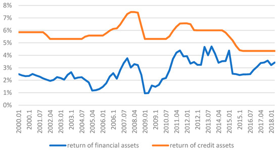
Figure 2.
Yield curve of credit and financial assets.
Given this context, we had several questions we wanted to address: (1) How should banks determine the holdings of these two types of assets with different yield characteristics when performing asset allocation? (2) What kind of dynamic adjustments do commercial banks make when asset prices in financial markets fluctuate? (3) How does the heterogeneity of commercial banks affect the configuration process? We provide answers to these questions in this article.
1.2. Contributions
Different from the existing literature, the innovation of this paper lies in the following points: First, according to the characteristics of the asset return rate, bank assets are divided into credit assets and financial assets, and then the impact of financial market fluctuations on bank asset allocation is analyzed. Second, this paper further investigates the impact of financial characteristics of commercial banks on the dynamic adjustment of bank assets. Third, considering the possible co-integration relationship between variables in this paper, a simple panel regression may fail to clearly identify the relationship between long-term equilibrium and short-term fluctuations. Therefore, this paper uses the panel error correction model to make an empirical analysis of the asset allocation of Chinese commercial banks.
Using the quarterly panel data of 23 listed commercial banks in China from 2002 to 2017, the empirical results of this paper show that the fluctuation of the return rate of two types of assets will affect the asset allocation of banks. Specifically, on the one hand, when the price of financial assets falls, which leads to the narrowing of the credit spread between the two types of assets, banks reduce transaction demand to prevent loss and reduce their holdings of financial assets, thus increasing the ratio of their credit assets to financial assets. On the other hand, rising benchmark lending rates leads to the increase in the credit financing cost of demanders, reducing the willingness of demanders to lend, and forcing the demander to obtain funds through other channels. This results in the decrease in the ratio of credit assets to financial assets. Furthermore, the financial characteristics of banks also influence the dynamic adjustment range of asset allocation. That is, the lower the reserve ratio and capital adequacy ratio, the smaller the impact of financial asset yield volatility on bank asset allocation.
2. Literature Review and Research Hypothesis
We review the related literature from two aspects: the factors influencing bank asset structure, and the impact of macro financial factors on company-level variables such as company capital structure. Then, the research hypotheses of this paper are formally proposed on this basis.
2.1. Impact of Macroeconomic Factors on Company-Level Variables
Korajczyk and Levy (2003) were the first to explore the impact of macroeconomic factors on a company’s capital structure. They classified companies into two categories: those subject to financing constraints and those that are not. For enterprises that are not subject to financing constraints, the target leverage ratio of the enterprise is characterized by the inverse economic cycle; otherwise, the target leverage ratio experiences a commensurate economic cycle. Enterprises that are not subject to capital constraints show equity financing preferences during periods of macroeconomic upswing, whereas those subject to capital constraints show debt financing preferences and therefore have higher debt ratios. Under the assumption that the trade-off theory had been established, Hackbarth et al. (2005) proved that the company’s capital structure adjustment is faster when the macroeconomic situation is better (Cook and Tang 2009). Cook and Tang (2009) used a series of macroeconomic indicators such as gross domestic product (GDP), credit spreads, and maturity spreads to measure the state of the economy, and empirically found, regardless of whether a company was subject to financing constraints, the company would thrive when macroeconomic conditions were favorable, and adjust its leverage ratios more frequently to approach target levels, thus verifying the theoretical model proposed by Hackbarth et al. (Su and Zeng 2009).
Su and Zeng (2009) used a nonlinear method, such as a panel score response, to investigate the impact of macroeconomic factors on capital structure changes of listed companies. The research results showed that the capital structure of listed companies changed following a significant countercyclical episode (Liu and Zeng 2014). When the macroeconomy shows prosperity or credit default risk rises, the company’s asset-to-liability ratio declines. However, credit rationing and stock market performance little impacted the capital structure. Liu and Zeng (2014) empirically analyzed the impact of macroeconomic factors, such as monetary policy, on banks’ risk tolerance capability using dynamic panel models. They used the non-performing loan ratio and the capital-to-risk (weighted) assets ratio (CRAR) as proxy variables of the risk-tolerance capability, and tested the correlation between the two by using the market interest rate and broad money supply (M2) as the price and quantity indicators of monetary policy, respectively. The results showed that the quantitative monetary policy indicators had a greater impact on the bank’s risk tolerance capability (Jin and Jia 2016).
Banks hold financial assets for two kinds of needs: trading needs and configuration needs. When the price of financial assets rises, the bank’s transactional demand for assets increases due to the profitability of short-term transactions. When the prices fall, from a long-term perspective, asset prices will return to normal levels in the future. Therefore, at this time, the bank’s demand for assets increases for the purpose of the long-term holdings of assets. Under the same market conditions, the two types of demand have different influences. In summary, we propose the following research hypotheses:
Hypothesis 1a (H1a).
When the price of financial assets declines (namely the rate of return increases), banks tend to reduce the trading demand for the purpose of mitigating loss, which causes banks to reduce the holding of financial assets, thus making the ratio of credit assets to financial assets rise.
Hypothesis 1b (H1b).
When the price of financial assets declines, banks increase the allocation demand for such assets in consideration of long-term asset holdings, leading to the increase in the proportion of such assets. As a result, the ratio of bank credit assets to financial assets reduces.
When the yield of credit assets rises, the supply and demand sides of the loan react differently. In the face of increasing yields, banks are willing to increase credit as credit providers. However, loan demanders, such as companies, will complete a cost-benefit analysis. The increase in loan financing costs reduces a company’s willingness to invest, or the company will instead try to obtain funds through other financing channels. Therefore, the change of the ratio of credit assets to financial assets depends on the strength of both the supply and demand sides of the market. Based on this, we propose the following research hypotheses:
Hypothesis 2a (H2a).
The increase of the benchmark interest rate on loans will prompt commercial banks to increase their credit supply, thus the ratio of credit assets to financial assets will rise.
Hypothesis 2b (H2b).
The rise in the benchmark interest rate of the loan will increase the financing cost of financiers, reducing the willingness of demanders to borrow, who then obtain funds through other financial markets, resulting in a decline in the ratio of credit assets to financial assets.
2.2. Factors Affecting Bank Asset Structure
The impact on a bank’s asset structure has mainly been studied from the perspectives of capital regulation, risk sharing, and financial disintermediation. For example, Jin and Jia (2016) studied the impact of leverage regulation on bank asset allocation. Previous studies suggested that leverage regulation causes banks to increase the proportion of bank risk assets, leading to an increase in the structural risk of assets (Zhang et al. 2013). However, they found that with Basel III setting leverage as a regulatory indicator, the impact of leverage on asset structure is subject to the spread of high- and low-risk bank assets. Zhang et al. (2013) examined the impact of bank risk tolerance on credit volume when studying the bank risk sharing channels of monetary policy. The results showed that the improvement in a bank’s risk tolerance exposure produced a significant increase in the number of loans (Zhou et al. 2017). Zhou et al. (2017) studied the impact of peer asset scale on bank risk-taking behavior, where the results showed that the increase in the peer asset scale significantly improved the bank’s risk-taking ability (Van den Heuvel 2007).
According to Van den Heuvel’s (2007) study, banks tend to reduce their holdings of risky assets in order to meet capital regulatory requirements, so that relatively high-risk loans become the main target of reductions (Wu 2011). Wu (2011) also supported the above viewpoints on the empirical analysis of commercial banks in China (Liu et al. 2016). Liu et al. (2016) studied the impact of capital constraints on bank balance sheets. Unlike previous research, they used the gap between the target and the actual capital adequacy ratio of each bank to define the degree of capital constraint instead of focusing on the specific reasons for the strength of capital constraints (Feng and He 2011). Feng and He (2011) extended the models of Gunjia and Yuan (2010) and analyzed the impact of listing financing and credit expansion on China’s monetary policy credit transmission channels. Their research results showed that capital adequacy ratio and credit scale were significantly and positively correlated. Listed financing has a significant positive effect on credit issuance, but the traditional monetary policy bank credit transmission channel is not obvious in China (Liu 2005). Liu (2005) examined the impact of capital adequacy ratio on loan interest rate elasticity. The results showed that banks with high capital adequacy ratios had lower loan interest rates. This shows that banks with insufficient capital have a greater impact on loan declines when they are regulated by tight monetary policy (Qian et al. 2014).
Qian et al. (2014) discussed the impact of financial disintermediation on the bank’s asset structure at the micro level. According to the empirical annual panel data of China’s listed banks, the financial disintermediation of the asset side prompted banks to increase the ratio of cash assets and reduce the proportion of loan allocations of commercial banks (Ren and Cheng 2015). At the macro level, Ren and Cheng (2015) used the VAR model to analyze the impact of various financial disintermediation factors on the asset–liability business of commercial banks. The research results showed that the bond issuance scale had a significant impact on loan issuance, whereas the scale of stock market financing and trust assets less affected the bank’s asset business (Zuo and Li 2016). When studying a bank’s stability, Zuo and Li (2016) used micro-bank data to study the impact of interest rate liberalization, income diversification, and the traditional deposit and loan business (Xu and Chen 2011). The empirical results showed that the deepening of marketization and the diversification of deposit and loan business reduced the operational stability of commercial banks.
Xu and Chen (2011) empirically tested how the three major instruments of China’s monetary policy affected credit supply behaviors through bank characteristics (Suo and Chen 2008). The results showed that both the liquidity capital adequacy ratio and bank asset size could affect the monetary policy’s effectiveness of bank credit channel. Suo and Chen (2008) built theoretical models of bank portfolio behavior, then used data to empirically test the cross-sectional effect of the propositional tight monetary policy on bank loan behavior introduced by the model; for banks with different asset sizes, the impact of monetary policy shocks on loan size is asymmetric (Tao 2016).
As the main financial intermediary institution in China, banks are subject to various regulatory constraints, such as capital adequacy ratio, deposit reserve ratio, and loan-to-deposit ratio. When a bank’s deposit reserve ratio is approaching the regulatory red alarm, the flexibility to decide where the funds flow is limited. The fluctuation of the yield of various assets is unlikely to affect the bank’s asset allocation behavior. At this time, the bank’s asset allocation decisions are often made to meet regulatory requirements. When the price of financial assets falls, banks should lower their share of financial assets. However, the risk weight of financial assets, such as securities, is lower than that of credit assets. If the proportion of credit assets increases and the share of financial assets decreases, the capital adequacy ratio should decline. When the bank’s actual capital ratio approaches the 10% capital adequacy requirement, it is increasingly difficult for banks to proactively manage credit assets and financial assets. Based on this, we propose the following:
Hypothesis 3 (H3).
With a lower bank deposit reserve ratio (liquidity index), the impact of financial asset prices on the ratio of bank credit to financial assets is smaller.
Hypothesis 4 (H4).
With a lower bank capital adequacy ratio, the reduction in the price of financial assets less affects the ratio of bank credit to financial assets.
3. Data Processing and Empirical Analysis
3.1. Variable Selection
According to the research hypotheses proposed above, dependent variable, independent variables and control variables selected in this paper are shown in the table below. Table 1 contains the sign and definition of each variables. Table 2 below shows the descriptive statistics of variables.

Table 1.
Definition of various variables.
Table 2.
The descriptive statistics of variables.
3.2. Data Source and Data Processing
The data required for the empirical test in this paper included micro-commercial bank financial data and macroeconomic data. For the financial bank data, we used the financial quarterly data of 23 listed banks. Limited by availability, we selected data between the first quarter of 2002 and the fourth quarter of 2017 from the Wind database. As each bank’s listing time was different, we used an unbalanced data panel. For macroeconomic data, pre-processing, including logarithm and seasonal adjustment, was required before empirical analysis. The time dimension of macroeconomic data was consistent with the bank’s financial data: from the first quarter of 2002 to the fourth quarter of 2017. The data were obtained from the China Macroeconomic Database, like Chang et al. (2016), and were adjusted according to the Chinese Statistical Yearbook and some other information. Finally, a time series model was used to obtain data for different frequencies of each macroeconomic indicator. Chang et al. (2016) used this database to analyze research topics related to the Chinese economy. Table 3 shows the correlation coefficient matrix for the main variables.
Table 3.
The correlation coefficient matrix for the main variables.
We used a long panel (small N, large T) for the panel data, to examine the long-term equilibrium relationship between the variables, which also showed a dynamic adjustment relationship in the short term. Therefore, testing the dynamic model before modeling was essential. The general steps of modeling involve the panel unit root test, panel co-integration analysis, and dynamic panel modeling.
3.3. Panel Unit Root Test
Similar to the unit root test method for univariate time series, there are many types of unit root test methods for panel data. Based on whether it is assumed that each section in the panel data has the same unit root process, the test methods can be classified into two categories. The first assumes the same section coefficients, such as the LLC test, the Breitung test, and the Hadri test. The second requires no such assumptions, such as the IPS test and the Fisher test. As our panel data were unbalanced, the Fisher test and IPS test were optional. As shown in Table 4, the Fisher test results were used as a reference for the stationarity test. The Fisher test provides the results of the stationarity test for each section in detail.
Table 4.
Panel unit root test results.
According to the test results, except for ROA, logarithmic real GDP, and reserve_ratio, the test results showed one unit root existed for raw data for other indicators, and the sequences after the first order difference were stable, which is the I(1) process. As regression of the same-order unsteady sequence might cause pseudo-regression problems, a co-integration test was needed.
3.4. Panel Co-Integration Test
The co-integration test method adopted in this paper is based on the error correction model proposed by Westerlund in 2007. In this method, if there is a co-integration relationship between variables, then in the error correction model based on these variables, the coefficients in front of the correction should be significantly different from zero. This method considers both the sequence correlation in the section and the correlation between the sections.
There are four test statistics. The first two (Gt and Ga) assume that the error correction speeds of the various sections are different, and the correction coefficient of each section is estimated by OLS; in the latter two (Pt and Pa), statistics are constructed based on the assumption that the error correction speed between the sections is the same. The definitions of the four test statistics are as follows:
where is the standard error obtained by OLS estimation. is the standard error used by Newey and West, which considers sequence correlation, and is the estimated value of which can be calculated by the OLS residual.
Gt and Pt are estimated without considering the assumption of sequence correlation, whereas Ga and Pa consider this assumption. The test results are shown in the following table. Only the Ga statistic supported the original hypothesis at the 10% level. The other three statistics opposed the hypothesis and suggested a co-integration relationship in the panel data. Therefore, the panel error correction model was adapted for potential co-integration. Considering the robustness of the empirical results in the robustness test, we used the deviation correction dummy variable least squares method (LSDVC) to test the dynamic panel model. The test results are shown in Table 5.
Table 5.
Panel cointegration test results.
3.5. Model Specification
According to the results of the unit root test, the ratio of credit assets to financial assets (b_qs), asset size logarithm (lnasset), capital ratio (zibenbilv), interbank seven-day interbank offered rate (R7dRepo), loan benchmark interest rate (LendingRatePBC1year), and broad money supply logarithm (logM2) followed the I(1) process. As a result, in the panel VEC model, the five variables above were all included in the long-term equilibrium relationship. The variables which we are interested in were added to the short-term dynamic adjustment.
In summary, to validate our proposed research hypothesis, two models were built. Model 1 was used to test Hypotheses 1 and 2, and Model 2 was used to test Hypotheses 3 and 4, as follows:
Model 1
Δb_qsit = b0 × (b_qsit−1 – a1 lnassetit−1 − a2 zibenbilvit−1 – a3 r7drepot−1
−a4 lendingratepbc1yeart−1 − a5 logm2t−1) + c1 Δb_qsit−1 + b1 Δlnassetit
+b2 Δroait + b3 Δreserve_ratioit + b4 Δzibenbilvit + b5 Δr7drepot
+b6Δlendingratepbc1yeart + b7 Δlogm2t + b8Δlogrealgdpt
+constant + eit
−a4 lendingratepbc1yeart−1 − a5 logm2t−1) + c1 Δb_qsit−1 + b1 Δlnassetit
+b2 Δroait + b3 Δreserve_ratioit + b4 Δzibenbilvit + b5 Δr7drepot
+b6Δlendingratepbc1yeart + b7 Δlogm2t + b8Δlogrealgdpt
+constant + eit
Model 2
Δb_qsit = b0 × (b_qsit−1 – a1 lnassetit−1 — a2 zibenbilvit−1 – a3 r7drepoit−1
−a4 lendingratepbc1yearit−1 − a5 logm2it−1) + c1 Δb_qsit−1
+b1 Δlnassetit +b2 Δroait + b3 Δreserve_ratioit + b4 Δzibenbilvit
+b5 Δr7drepot + b6 Δlendingratepbc1yeart + b7 Δreserve_ratiot × r7drepot
+b8 Δzibenbilvit × r7drepot + b9 Δlogm2t + b10 Δlogrealgdpt + constant + eit
−a4 lendingratepbc1yearit−1 − a5 logm2it−1) + c1 Δb_qsit−1
+b1 Δlnassetit +b2 Δroait + b3 Δreserve_ratioit + b4 Δzibenbilvit
+b5 Δr7drepot + b6 Δlendingratepbc1yeart + b7 Δreserve_ratiot × r7drepot
+b8 Δzibenbilvit × r7drepot + b9 Δlogm2t + b10 Δlogrealgdpt + constant + eit
3.6. Empirical Test: Model 1
Three main estimation methods are available to estimate the panel error correction model: the mean group (MG) estimator, the fixed effects (FE) estimator, and the pooled mean group (PMG) estimator. The fixed-effect estimator assumes that the long-term and short-term slope coefficients of the respective sections are the same, so that with the estimator utilized, the time sequence data of the respective sections can be mixed and used. The inter-group estimator assumes that the long-term and short-term slope coefficients of each section are different, so the time sequence data of each section are used alone, and the coefficients of each section are estimated separately. Finally, the average value between the groups is taken to obtain the estimated coefficient of the whole sample. The assumptions for the estimators between the mixed groups are somewhere in between. It assumes that the long-term slope coefficients of the various sections are the same, but the short-term slope coefficients are different. Furthermore, the maximum likelihood estimation method can be used to obtain the estimator between the mixed groups.
Table 6 shows the estimation results obtained using the three different methods described above. Columns (1)–(3) are the FE estimator, the MG estimator, and the PMG estimator, respectively. In the three columns of results, the ec values, representing the error fixing speed, are both negative and significantly non-zero, indicating that a co-integration relationship does exist in the model.
Table 6.
Results of the regression analysis of Model 1.
Among the explanatory variables related to bank characteristics, asset size, reserve ratio, and capital-to-asset ratio all had a significant impact on the bank’s asset ratio. Among these, the estimated coefficient of asset size was negative, which was consistent with the research results of Xu and Chen (2011), indicating that the larger the bank’s assets, the smaller the proportion of credit and financial assets and the more banks invest in the finance market. This might result from the fact that we defined interbank funds as financial assets, which quickly developed prior to 2015, leading to a relative decline in the ratio of credit to financial assets. The reserve ratio measures the bank liquidity indicator, and the capital asset ratio represents the bank’s capital adequacy level. Positive values of both of their coefficients indicate that the better the liquidity of the bank, the lower the capital constraint, and the more active the credit, which then leads to a higher ratio of credit to financial assets.
Among all the macroeconomic indicators, in the long term, an increase in the broad money supply (M2) indicates loose current monetary policy and expansion in both credit assets and financial assets. However, if the ratio between the two increases, monetary policy will have an asymmetric impact on these two types of assets. In the short term, although the M2 coefficient was positive, it was not insignificant, which might be related to the longer transmission time lag of monetary policy. In the study of this paper, the impact of real GDP on the asset side of banks was a more interesting question. In the unit root and co-integration tests in the previous section, we rejected the assumption that the logarithmic real GDP and bank asset allocation had a long-term equilibrium relationship, so the horizontal term of logrealgdp was not included in the long-term equilibrium equation—only its differential term was used in the short-term dynamically adjusted equation. Furthermore, in the PMG estimator, the coefficient of the differential logrealgdp was significantly positive, which indicates that the actual macroeconomic expansion stimulates the bank’s loan issuance. Compared to financial assets, loan yields are higher and riskier. When the economy shifts from recovery to prosperity, the productive enterprises in need of financing stimulate bank credit from the demand side. For banks, a prosperous economy means better production and operation of enterprises and lower risks of loans, thus the credit supply of banks is promoted.
3.7. Empirical Test: Model 2
Table 7 reflects the empirical tests performed on Hypotheses 2 and 3. For short-term dynamic adjustment, the model adds the cross terms ‘cross2a’ and ‘cross3a’, which are the product terms of the financial asset’s return rate and reserve ratio, and the financial asset’s return rate and the capital share, respectively. According to previous research hypotheses, the coefficients of the two cross terms should be positive. The regression results in the table confirm this; regardless of the estimation method being used, the estimated coefficients of cross2a and cross3a were positive numbers. The estimated coefficient cross3a was significant under the three estimators, showing that the higher the capital-to-asset ratio, the more sensitive the bank’s asset allocation to the price fluctuations of financial assets. When the asset price of the financial market declined (the rate of return increased), the higher the capital-to-asset ratio and the looser the capital constraints. Therefore, the funds more freely allocated to financial assets can be transferred to credit assets without the constraint of adequate regulatory requirements. The estimated coefficient cross2a was significant in both FE and MG estimation, but not significant in the PMG estimator. To a certain extent, this shows that the sensitivity of bank asset allocation to financial market volatility will be affected by the ratio of the deposit reserve ratio. Cash and deposits in central banks are assets with the most liquidity. When banks try to respond quickly to the external market environment changes, using excess reserves and cash is the least costly option.
Table 7.
Results of the regression analysis of Model 2.
In the empirical test results, the addition of the cross-term did not much influence the coefficients of the original interbank seven-day offered rate and the loan benchmark interest rate. R7dRepo and LendingRatePBC1year were still significant under the PMG estimator and the sign of the coefficient was consistent with our previous deduction. To a certain extent, this shows that the empirical results of this paper were robust.
3.8. Robustness Test
The dynamic panel data are provided in the form of long panels and short panels. If panel N is large and T is small, it is a short panel, otherwise it is a long panel. When N is large, the estimation method based on IV or GMM is unbiased. Since the panel data in this paper were a long panel, deviations may have occurred in the estimation method using IV or GMM (Chen 2010). Kiviet (1995) used the Monte Carlo simulation method to obtain the following results. In the case of a small N, the deviation-corrected LSDVC method could correct the estimated deviation by more than 90%. For either the deviation correction or the mean square error index, LSDVC was better than the differential GMM or system GMM. Therefore, we used the bias correction LSDV method, also known as LSDVC, to test the robustness of the model.
Given our four research hypotheses above, the following two empirical models were built in the robustness test. Model 3 was used to test Hypotheses 1 and 2, and Model 4 was used to test Hypotheses 3 and 4. Interactive items were added to Model 4 based on Model 3, as follows:
Model 3
b_qsit = a1 b_qsit−1 + a2 lnassetit + a3 roait + a4 reserve_ratioit + a5 zibenbilvit
+ a6 r7drepot + a7 lendingratepbc1yeart + a8 Δlogm2t + a9 Δlogrealgdpt
+ ui + eit
+ a6 r7drepot + a7 lendingratepbc1yeart + a8 Δlogm2t + a9 Δlogrealgdpt
+ ui + eit
Model 4
b_qsit = a1 b_qsit−1 + a2 lnassetit + a3 roait + a4 reserve_ratioit + a5 zibenbilvit
+a6 r7drepot + a7 lendingratepbc1yeart + c1 reserve_ratiot × r7drepot
+c2 zibenbilvit × r7drepot + a8 Δlogm2t + a9 Δlogrealgdpt + ui + eit
+a6 r7drepot + a7 lendingratepbc1yeart + c1 reserve_ratiot × r7drepot
+c2 zibenbilvit × r7drepot + a8 Δlogm2t + a9 Δlogrealgdpt + ui + eit
In order to reduce the endogeneity problem caused by two-way causality, the models use the lag phase of the explanatory variable, such as asset size, reserve ratio, and capital adequacy ratio, as the instrumental variable to enter the empirical model; L1 is appended to the variable name, indicating the lag period of the variable. The empirical results of the LSDVC method are shown in Table 8 Three columns of results are presented. The first column presents the estimations of the traditional fixed-effects model, the second column presents the Arellano-Bond (AB) differential GMM estimator as the initial value for the bias correction, and the third column presents the results of using the Blundell-Bond (BB) system GMM estimator as the initial value of the deviation correction. The standard error of the calculation coefficient of bootstrap was used, and the sampling frequency was set to 50 times.
Table 8.
Robustness test of Model 3.
The basis for using the AB difference estimator or the BB system estimator was the coefficient size of the interpreted variable (L.b_qs). The coefficient of b_qs was large (about 0.8), which means that b_qs had a strong sequence correlation. The use of the horizontal lag term as the instrumental variable of the difference term in the difference equation produces a weak instrumental variable. Therefore, the BB system GMM estimator was a better choice than the AB differential GMM estimator.
The two tables above present the empirical results of Model 1 and Model 2, respectively. Our focus was the significance of the coefficient of return on financial assets and the rate of return on loans in the third column. According to the empirical analysis of the third column in Table 7, the coefficients of R7dRepo and LendingRatePBC1year were significant, once again confirming hypotheses H1a and H2b. According to Table 9, the estimated coefficients of the cross terms cross2a and cross3a were both significantly positive. The estimated value obtained by the LSDV method was consistent with the previous results obtained by the panel error correction model, indicating that the empirical results of this paper were robust.
Table 9.
Robustness test of Model 4.
4. Conclusions
With the continuous development of interest rate marketization, traditional credit spreads have narrowed. Finding an alternative strategy to traditional credit business, to broaden the scope of business and profit sources, and to realize the sustainable development of the banking industry, are common problems faced by various commercial banks. Financial disintermediation poses a challenge to China’s bank-based indirect financing model. The efficiency of production and transmission of information in the financial market continue to increase, and investors can easily determine the credit status of borrowers. Compared with the costlier indirect financing model, an improving financial market provides an alternative for borrowers who are interested in direct finance.
The comprehensive management of the banking industry provides a new strategic direction for the development of banks. This strategy will utilize existing customer resources, business branches, and specialized financial technologies of the bank to develop a comprehensive “stock, debt, loan, broker, and customer” operation framework. Compared with the situation in the late 1990s and early 2000s, banks’ asset businesses have undergone tremendous changes, and the range of available asset allocation decisions has become more abundant. For example, banks have become the most important players in the bond market, banks have participated in the primary equity market by setting up holding subsidiaries, and the off-balance sheet funds of banks can flow into the secondary stock market or the real estate market through services such as trust channels.
In summary, banks’ funds are widely involved in various financial markets through all kinds of channels. This provides a channel for banks to disperse credit risk. However, as bank funds and capital markets become increasingly integrated, the risks inherent in financial markets are conducted in accordance with the bank’s balance sheet. Compared with the fluctuation of credit interest rates under regulation, the fluctuation of market prices—as a concentrated reaction of market information—necessarily contains the market’s perception of risk.
As a result of many factors, including the incompleteness of the interest rate dual track system due to the immaturity of marketization, two main types of bank assets have different yield characteristics: credit assets and financial assets. The higher the yield of credit assets, the lower the yield of financial assets; as the yield of credit assets fluctuates less, the yield of financial assets fluctuates greatly with the market environment. Facing the impact of financial markets, banks will dynamically adjust the ratio of the two types of assets. Asset adjustments are also affected by the heterogeneity of banks, in terms of factors such as capital adequacy and liquidity.
Empirical studies showed that when the price of financial assets declines (i.e., the rate of return rises), banks’ transaction demands outweigh the allocation demands. In order to stop or mitigate loss, banks will reduce the holdings of financial assets, thereby increasing the ratio of bank credit assets to financial assets. Although the increase in the benchmark interest rate of loans could prompt banks to expand credit supply, it will also increase the borrower’s credit financing costs, thus reducing the borrowers’ willingness to lend and obtain funds through other financial markets, resulting in the decrease in the ratio of credit assets to financial assets. In addition, bank characteristics also affect the sensitivity of banks to changes in the assets’ return. When the bank’s deposit reserve ratio (liquidity index) is lower, the impact of financial asset prices on the ratio of bank credit to financial assets is weaker; when the bank’s capital adequacy ratio is lower, the decrease in the price of financial assets has a weaker impact on the ratio of bank credit to financial assets.
Author Contributions
This paper was written by K.H., Q.Y. and C.L. K.H. and Q.Y. conceived the idea and designed the structure of the paper. C.L. collected the data and completed the draft.
Funding
This research received no external funding.
Conflicts of Interest
The authors declare no conflicts of interest.
References
- Chang, Chun, Kaiji Chen, Daniel F. Waggoner, and Tao Zha. 2016. Trends and Cycles in China’s Macroeconomy. NBER Macroeconomics Annual 30: 1–84. [Google Scholar] [CrossRef]
- Chen, Qiang. 2010. Advanced Econometrics and Stata Applications. Beijing: Higher Education Press. [Google Scholar]
- Cook, Douglas O., and Tian Tang. 2009. Macroeconomic conditions and capital structure adjustment speed. Journal of Corporate Finance 16: 73–87. [Google Scholar] [CrossRef]
- Feng, Ke, and Li He. 2011. The Impact of Banking Financing and Credit Expansion on the Transmission Mechanism of Monetary Policy in China. Economic Research 46: 51–62. [Google Scholar]
- Gunjia, Hiroshi, and Yuan Yuan. 2010. Bank Profitability and the Bank Lending Channel: Evidence from China. Journal of Asian Economics 12: 129–41. [Google Scholar] [CrossRef]
- Hackbarth, Dirk, Jianjun Miao, and Erwan Morellec. 2005. Capital structure, credit risk, and macroeconomic conditions. Journal of Financial Economics 82: 519–50. [Google Scholar] [CrossRef]
- Jin, Yuying, and Songbo Jia. 2016. Research on the Influence of the Introduction of Leverage Regulation on the Asset Structure of Commercial Banks. Studies of International Finance 350: 52–60. [Google Scholar]
- Kiviet, Jan F. 1995. On bias, inconsistency and efficiency of various estimators in dynamic panel data models. Journal of Econometrics 68: 53–78. [Google Scholar] [CrossRef]
- Korajczyk, Robert A., and Amnon Levy. 2003. Capital structure choice: Macroeconomic conditions and financial constraints. Journal of Financial Economics 68: 75–109. [Google Scholar] [CrossRef]
- Liu, Bin. 2005. An Empirical Study of the Impact of Capital Adequacy Ratio on Banks Loans. Journal of Finance 11: 18–30. [Google Scholar]
- Liu, Shengfu, and Cheng Zeng. 2014. Monetary Policy Regulation, Bank Risk Taking and Macroprudential Management—An Empirical Analysis Based on Dynamic Panel System GMM Model. Nankai Economic Studies 5: 24–39. [Google Scholar]
- Liu, Xiaofeng, Dapeng Zhu, and Wenfan Huang. 2016. An Empirical Study of the Impact of Capital Constraints on the Balance Sheet of China’s Commercial Banks. Studies of International Finance 5: 61–71. [Google Scholar]
- Qian, Wei, Sen Cao, and Cong Jiang. 2014. Empirical Study on the Influence of Financial Disintermediation on the Asset Structure of Commercial Banks. Zhejiang Finance 7: 45–48. [Google Scholar]
- Ren, Biyun, and Yulun Cheng. 2015. The Dynamic Impact of Financial Disintermediation on the Impact of China’s Commercial Banks’ Asset and Liability Business—An Empirical Study Based on VAR Model. Journal of Central University of Finance & Economics 3: 26–33. [Google Scholar]
- Su, Dongwei, and Haijian Zeng. 2009. Macroeconomic Factors and Changes in Corporate Capital Structure. Economic Research 44: 52–65. [Google Scholar]
- Suo, Yanfeng, and Jiming Chen. 2008. Asset Size, Capital Status and Commercial Bank’s Portfolio Behavior—An Empirical Analysis Based on Panel Data of China’s Banking Industry. Journal of Financial Research 6: 21–36. [Google Scholar]
- Tao, Zha. 2016. China’s Macroeconomy: Time Series Data. Available online: http://www.tzha.net/code (accessed on 11 December 2018).
- Van den Heuvel, Skander J. 2007. The welfare cost of bank capital requirements. Journal of Monetary Economics 55: 298–320. [Google Scholar] [CrossRef]
- Wu, Wei. 2011. The Impact of Capital Constraints on the Asset Allocation Behavior of Commercial Banks—An Empirical Study Based on Data of 175 Commercial Banks. Journal of Financial Research 4: 65–81. [Google Scholar]
- Xu, Mingdong, and Xuebin Chen. 2011. Characteristics of China’s Micro Banks and Bank Loan Channels. Management World, 24–38. [Google Scholar]
- Zhang, Qiang, Yifeng Qiao, and Zhang Bao. 2013. Is There a Bank Risk-Taking Channel for China’s Monetary Policy? Journal of Financial Research 8: 84–97. [Google Scholar]
- Zhou, Zaiqing, Yi Gan, and Yue Hu. 2017. Characteristics and Risk-Taking Behavior of Commercial Banks’ Interbank Assets—An Empirical Analysis Based on GMM of China’s Banking Dynamic Panel System. Studies of International Finance 7: 66–75. [Google Scholar]
- Zuo, Yuehua, and Xiaoxin Li. 2016. Interest Rate Marketization, Bank Diversification and Bank Robustness—An Empirical Analysis Based on Unbalanced Panel Data of China’s Commercial Banks from 2007 to 2014. Investment Research 35: 99–107. [Google Scholar]
© 2019 by the authors. Licensee MDPI, Basel, Switzerland. This article is an open access article distributed under the terms and conditions of the Creative Commons Attribution (CC BY) license (http://creativecommons.org/licenses/by/4.0/).