Article

Using Grey Incidence Analysis Approach in Portfolio Selection

Faculty of Economics and Business, University of Zagreb, 10000 Zagreb, Croatia
*
Author to whom correspondence should be addressed.
Int. J. Financial Stud. 2019, 7(1), 1; https://doi.org/10.3390/ijfs7010001
Submission received: 4 November 2018 / Revised: 20 December 2018 / Accepted: 20 December 2018 / Published: 23 December 2018

Abstract

:
Due to the development of financial markets, products, financial and mathematical models, portfolio selection today represents a comprehensive set of activities. Investors take into consideration many different factors, such as the market factors, return distribution characteristics and financial statements information. This research applies a Grey Relational Analysis (GRA) approach to evaluate the performance on a sample of stocks by taking those different factors into consideration. The results based upon a sample of 55 stocks for the trading year 2017 on the Croatian capital market show that using GRA approach in portfolio selection provides useful guidance for investors when making investment decisions, and better portfolio results in terms of risk and return are reachable compared to an equally weighted portfolio benchmark.

1. Introduction

Portfolio selection today represents a very difficult task in portfolio management due to many investment possibilities on the financial markets, many factors influencing the investors’ decisions and constant dynamic changes on the markets as well. Investors have to make daily decisions based upon different information. Thus, a quality decision making process should be supported with quantitative modelling which can ease this process and achieve investment goals. Utility function theory has been developed regarding an investor’s utility being based upon first m moments of return distributions (see Jurczenko and Maillet 2005) explaining that investors make their decisions based upon those distribution moments. Moreover, many studies have shown that financial ratios data are useful in portfolio management as well (Chen and Thomas 1981; Singh and Schmidgall 2002). In that way, many different methodologies in mathematics and econometrics have been developed in order to provide some of the answers to investor’s questions regarding stock performance and portfolio selection. Some of the most popular approaches to deal with large amounts of information include Data Envelopment Analysis (see Chen 2008 or Dia 2007), Multicriteria Decision Analysis (Steuer et al. 2008 or Edirisinghe and Zhang 2007) and Multivariate analysis (clustering, principal components analysis and similar approaches, see Korzeniewski 2018). However, a relatively unknown and new approach is the Grey Relational Analysis (GRA) approach. This methodology, i.e., the wider term Grey Systems, was firstly developed in the field of modelling uncertain systems and it was applied over different areas such as decision making processes, ecological, hydrological, geological and similar systems (see Liu et al. 2016 for the history development and different areas of applications). The novelty and contribution of this research is applying the GRA approach in the decision making process in portfolio selection, since this approach is found to be extremely rare in financial applications, especially when making decisions on the structure of the stock portfolio. The results from GRA approach ranking of stocks is used for the simulation of portfolio investing, an approach which is also rarely found in applications. Moreover, the contribution of this study compared to existing ones is in providing the rationale of why we include chosen variables, i.e., factors in the modelling procedure, based upon financial theory and empirical findings over decades. This is in the majority cases ignored in the empirical applications.
Thus, the main goal of this study is to empirically evaluate market and financial statement data on a sample of stocks by using the GRA approach in order to obtain information on whether this approach could be applicable to portfolio selection. This will be achieved by comparing the portfolios which are a result from taking into consideration the best stocks from the GRA ranking system in sample and by comparing the out of sample performances of simulated portfolios in the empirical analysis. The GRA approach of evaluating performance has several advantages compared to other approaches such as Data Envelopment Analysis, Analytic Hierarchy Process and other approaches: it is not sensitive to data transformations, easier estimations are available, and straightforward interpretations can be made, etc. (Wei 2011). Thus, two main research questions are as follows. First, can the Grey Relational Analysis provide a useful guidance for investors when making investment decisions? This question asks if results given with one number from the GRA provides useful information on how to form stock portfolios. The second question is whether portfolios formed based upon the GRA approach can provide better results in terms of risk and return compared to a simple benchmark (equally weighted portfolio).
The rest of the paper is structured as follows. The second section deals with previous related research. The third section describes the methodology used in the study. Results and discussion are given in the fourth, fifth and sixth sections. The final section concludes the paper.

2. Previous Research

By analyzing previous existing research which applies the GRA approach in finance, it can be seen that there is a great scarcity of research in this area. The majority of the applications were made in different fields (see Liu and Lin 2010 for details).
Huang et al. (2008) combined weight clustering model with the K-means Clustering approach and the Grey Systems Theory with the Rough Set theory in order to create automated stock market forecasting with portfolio selection on the Taiwanese market for the period 1Q2003—4Q2016. Authors thus apply a dynamic analysis in which in every quarter they collect financial data on selected stocks and cluster them by using K-means clustering. Finally, the GRA approach is used to rank the stocks and include the portfolios. The results indicate that such formed portfolios obtain significant returns over the observed period. It can be seen in this research that authors observe those investors who only aim at the greatest returns possible. Several financial ratios were chosen in the research and rationale is based upon investment principles advocated by W. Buffett, as authors’ state. Huang and Jane (2008) extended this research by combining Fuzzy C-means theories with Variable Precision Rough Set theory when comparing stocks with the Average Autoregressive Exogenous prediction model of the future stock market movements. The GRA analysis was also used to specify the weighting of the selected stocks, with the same approach as in the previous paper, to achieve maximum rate of return. Again, a dynamic analysis was performed for the period 2004 until 2006 based upon quarterly data and financial ratios. Here, the authors do not state why they used the financial data which was included in the empirical research. However, the authors conclude based upon the results that such combination of the aforementioned approaches leads to achieving great portfolio rate of returns.
Li et al. (2010) combine the AHP (Analytic Hierarchy Process) methods for the stock selection on 8 listed companies within the steel industry on the Chinese stock market. There is no time span stated in the research, and authors use the following factors to rank stocks: profitability (profit margins and net profit margins), profit and sales growth rates, earnings per share, price to earnings ratio, solvency ratios and operating ability ratios. The approach in this study is to obtain weights via AHP for the second step of GRA and conclude that the results are promising. However, no investment decisions were applied in order to compare portfolio results. Jane and Huang (2013) focus again on the automatic stock selection mechanism, this time by combining Artificial Neural Network with the GRA modelling. All companies listed on the Taiwanese market in the period from November 2008 until April 2013 were used for comparison purposes. The results were very promising with obtaining extraordinary results as in Huang and Jane (2008). Salardini (2013) combines the AHP and GRA approaches on the sample of 16 stocks on Tehran Stock Exchange in year 2010. Both approaches were used in order to obtain optimal weights in the ranking system. Stocks were ranked based upon several factor, but no explanation is given for the usage of chosen variables. Mohammadi Pour et al. (2016) is one of the last to apply GRA analysis on the stock selection process. Authors compared 14 stocks from the Tehran Stock Exchange for the period 2009–2014. In total 4 financial ratios were used in the study (with no explanations on why those) and rankings were made and compared to the Johnson forecasting ranking. Results indicated similar ranking results for both methods.
As can be seen from the literature overview, not many studies exist within this field. Moreover, portfolio selection as in terms of risk diversification was not observed as well. Finally, not many papers include explanations and rationale from the financial theory standpoint which factors should be included in the analysis. This is why this research is trying to fill that gap.

3. Methodology

For describing the methodology used in this study, we follow Liu and Lin (2006, 2010). This methodology was firstly developed in Deng (1982) and since then it was applied in different areas of research (for overview, please see Deng 1989; Liu et al. 2016). This approach of modelling is used to build a ranking system of alternatives in order to choose the best one. Denote with (xi(1), xi(2), ..., xi(n)) the behavioural sequence of the k-th factor, k ∈ {1, 2, …, n} for observed alternatives i ∈ {1, 2, …, m}. All of the data can be formatted into the matrix X:
X = [ x 1 ( 1 ) x 1 ( 2 ) x 1 ( n ) x 2 ( 1 ) x 2 ( 2 ) x 2 ( n ) x m ( 1 ) x m ( 2 ) x m ( n ) ]
The data is normalized so a comparability sequence can be obtained: (yi(1), yi(2), …, yi(n)), with normalization accordingly to rules of data being the greater (larger) the better:
y i ( k ) = x i ( k ) min i   x i ( k ) max i   x i ( k ) min i   x i ( k ) ,
the smaller the better:
y i ( k ) = max i   x i ( k ) x i ( k ) max i   x i ( k ) min i   x i ( k ) ,
or the closer to the desired value x*(k) the better:
y i ( k ) = | x i ( k ) x * ( k ) | max i   x i ( k ) x * ( k ) .
Normalization could be made by dividing each value for factor k by the first value x1(k) as well. When using expressions (2) and (3) to normalize data, every new value will be within the interval [0, 1]; and the greater the normalized value is, the closer is the original value to the minimum or maximum, depending on the criteria. In order to calculate the Grey Incidence Index, absolute differences are calculated compared to the referent value y*(k):
Δ y i ( k ) = | y * ( k ) y i ( k ) | .
Kuo et al. (2008) define the reference sequence as all values y*(k) being equal to one. The Grey Relational Coefficient is calculated as:
G i ( k ) = Δ min + p Δ max Δ y i ( k ) + p Δ min ,
where p is the distinguishing coefficient, 0 ≤ p ≤ 1; Δ min = min { Δ y 1 ( k ) , , Δ y m ( k ) }   k ; Δ max = max { Δ y 1 ( k ) , , Δ y m ( k ) }   k . Finally, the Grey Relational Degree (Relational Grade) for each alternative is a weighted average of relational coefficients for different factors:
r i = i = 1 n w i G i ( k ) , i ,
where weights wi satisfy the condition: i = 1 n w i = 1 . The Grey Relational Grade in (7) for each alternative is interpreted as the degree of similarity between the reference sequence of y*(k)-s and the alternatives being compared to it. In some literature it is interpreted as the correlation coefficient. Thus, the greater the value of ri for an observed alternative, the better the performance it is considered to have compared to others. As it can be seen, this approach is relatively simple, straightforward and directly interpretable. More details can be seen in Liu et al (2016).

4. Empirical Results

4.1. Data Description and Rationale for Used Factors

For the purpose of the empirical analysis, daily price data on most liquid1 stocks on the Croatian stock market, Zagreb Stock Exchange (ZSE 2018) was collected for the year 2017. Most liquid stocks are observed in order to have as much as data possible. In that way, the sample consists of 55 stocks in total. Moreover, additional data on return series was collected in the first half of 2018 for the out of sample calculations and comparisons (see Section 5). Moreover, several financial ratios for each stock have been obtained from financial statements of 2017 as well. In that way, the analysis can be undertaken based upon the newest data possible. Thus, the analysis will include ranking of the stocks based upon the return distribution characteristics, as well as on financial statements of each company. Based upon the daily prices, daily continuous returns were calculated and average return for the 2017 was calculated for each stock. Next, standard deviations as a risk measure and coefficients of asymmetry and kurtosis were calculated as well for each stock. It is assumed that investors base their decisions on investing based upon the first m moments of return distribution. As Arditti (1967) discussed: investors prefer positive skewness of returns as a result of decreasing absolute risk aversion; and the famous theorem of Müller and Machina (1987, p. 351) which states that investors with von Neumann–Morgenstern utility functions rank probability distributions on the basis of their first m absolute moments. Based upon the investor’s utility function theory, in the analysis we assume that investors prefer higher odd moments of return distribution (first and third moments: average return and skewness), whilst they prefer smaller event moments (second and fourth moments: standard deviation and kurtosis). For more details on investor’s utility functions discussion and preferences towards the m moments of return distribution please see Arditti and Levy (1975), Athayde and Flôres (1997), Hwang and Satchell (1999), Briec et al. (2006), Jurczenko and Maillet (2005), Jondeau and Rockinger (2006) or Gardijan and Škrinjarić (2015).
Two liquidity measures used in the study, trading volume and number of transactions, are referred to as market measures. Previous literature finds negative relationship between the liquidity premium and stock returns (Datar et al. 1998; Pástor and Stambaugh 2003; Liu 2006; Hur et al. 2018; Hur and Chung 2018). Thus, the approach in this research is that investors aim for lower liquidity in order to obtain illiquidity premiums. Inclusion of financial statements data is based upon previous research which finds that there exist differences in stock returns depending upon financial ratios. Basu (1977) was one of the first studies to find that firms with a small price to earnings (PE) ratio had higher returns compared to other firms on the US market in the long term. Shiller (2005) showed that long-term investors should focus on lower PE ratios, whilst in short term it is possible to obtain excess returns with higher PE ratios. Since we observe a short-term in this study, we focus on greater PE ratios. Book to market ratio (BM) was extensively studied over the last couple of decades. Banz (1981) and Reinganum (1981) were some of the first studies to conclude that smaller stocks have greater returns compared to bigger ones. This stimulated Fama and French (1992, 1993, 1995, 1996) to include this ratio into their famous 3-factor model and found a strong positive effect of BM ratio on cross-sectional stock returns. That is why we are aiming for a greater value of this ratio in the analysis. Furthermore, Wu (2000) conducted a survey of institutional and individual investors and found that earnings per share (EPS), return on assets (ROA) and liquidity ratios are some of the most used financial ratios when investors make their investment decisions in practice. This was confirmed in Muhammad and Scrimgeour (2014), who add return on equity (ROE) to this list as well and conclude that these ratios give information to investors on effective and efficient usage of the firm’s assets and equity in order to generate profits. Moreover, investors should aim towards greater value of mentioned ratios due to them being a proxy for performance measurement of firms and efficiency of their management. That is why investors should aim greater values of EPS, ROA and ROE (evidence was found as well as in Dimitropoulos and Asteriou (2009) and Palepu and Healy (2010)). Finally, the positive relationship between the Dividend per Share (DPS) ratio and expected returns has been found very early in the literature in work of Fama and Schwert (1977) and Campbell (1987); and has been continuously confirmed over the years as well in Fama and French (1988), Campbell and Shiller (1988), Kothari and Shanken (1997) or Lewellen (2004).
Table A1 in Appendix A depicts the used factors in the study, with their abbreviations in brackets and the preferred values of each factor. If investor should prefer higher value, a plus sign is added; and opposite is true for those factors which should be lower. Table 1 shows the average, minimum and maximum value of each factor in the analysis. It can be seen that the values vary significantly. However, due to the many factors upon which to base investment decisions, the GRA approach seems appropriate.

4.2. Results in Sample

Firstly, based upon the signs in Table A1 (in Appendix A), each factor was normalized by using Formulas (2) and (3). The distinguishing coefficient was chosen ranging from 0.1 to 0.9 and the results of the degrees of grey incidence for each stock. Since the ranking does not change with respect to the distinguishing coefficient (see Figure 1), Table 2 is showing Grey relational grades for the value of the coefficient being 0.5. This could be interpreted as the correlation between the performances of each stock with respect to all factors to the optimal value of 1 for each factor. Moreover, here we have chosen equal weights for all of the factors in the analysis as a starting point. This means that it is assumed that investors are regarding all of the information (factors) on stocks in an equal manner. It can be seen that the best stocks in terms of performance in Table 2 are TUHO, MDKA, ATLN, LKRI and LPLH, due to them having the greatest values of degree of incidence. The worst performance had LEDO, OPTE, DDJH, DLKV and INGR. This conclusion is robust when changing the distinguishing coefficient, as it can be seen on Figure 1. Thus, from an initial larger sample of stocks available, investor can use this information to narrow his set of interesting stocks to evaluate further or to invest in the best performing stocks.
In order to obtain more information on the usefulness of using the GRA approach, an additional ranking was made based upon several other criteria. In the first scenario it is assumed that an investor regards only the first two moments of return distribution equally and gives them equal weight. Moreover, the investor ignores all other factors. This scenario is denoted “2 moments”. Other scenarios include: investor equally weights only the first three moments (“3 moments”); first four moments (“4 moments”); only the financial ratios data (“only financial”); major weight is given to the risk (50%, whilst other 50% is equally distributed to all other factors; “risk”); major weight is given to the return (50%, whilst other 50% is equally distributed to all other factors; “return”) and final scenario in which 70% of the weight is given to return distribution moments, whilst other 30% to other factors (named “0.7 moments; 0.3 other”). Thus, the whole procedure of calculation was performed again and the Grey incidence indices are compared on Figure 2. Although it seems that for many cases the ranking remained the same, some major differences arise when investors change their preferences. The detailed ranking is shown in the Appendix A, in Table A3. Some major differences occur for, e.g., stock ZVZD, which was ranked the best according to the scenarios “3 moments” and “return”, but is almost the worst (53 rank out of 55) when taking into account scenario “risk”. Thus, the ranking will depend upon investor’s preferences and subjective goals.
We wanted to obtain information whether this ranking system can provide a successful portfolio selection in terms of risk and return, by constructing efficient frontiers in terms of the Markowitz portfolio (Markowitz 1952, 1959). Firstly, an original efficient frontier was constructed based upon the whole sample in order to compare how closely the investor can approach this frontier with the analysis of GRA approach. This is depicted on Figure 3 and denoted with “efficient frontier”. This original frontier was constructed based upon varying the risk in the Markowitz (1959) model from the minimum variance portfolio until the portfolio with the maximum return.
Next, based upon the rankings on Figure 2, several frontiers were constructed as a second step of the whole analysis. Notation is the same as on Figure 2. However, these frontiers are not efficient in terms of the Markowitz model, due to them being constructed based upon several points: the first point was constructed such that weights to individual stocks were constructed based upon the grey incidence indices. Every weight is equal to the value of the individual index divided by the total sum. In that way, all of the stocks entered the portfolio. The second point was constructed by giving equal weights to the first 3 best stocks based upon the grey indices. The third point was constructed by giving equal weights to the first 5 best stocks based upon the same indices. In that way, we wanted to observe how the point changes from the starting value when all of the stocks are included in the portfolio. By undertaking this analysis, we can obtain information if the portfolio goes closer to the Markowitz efficient frontier or away from it.2 As can be seen on Figure 3, interesting results arise, depending upon what investor takes into consideration. The best approach in this analyzed sample was for all of those scenarios which included portfolio moments, due to these frontiers expanding towards the original efficient frontier. The worst performance was obtained for only financial data. This means that in this observed period, if investors based their analysis mostly on the return distributions, they could have formed such portfolios to obtain good results in terms of portfolio risk and return. On the other hand, the inclusion of financial data did not result in desiredoutcomes. However, it can be seen as well that when the portfolios are compared to the equally weighted portfolio (denoted with “equally w portfolio”), investor can achieve better results (greater return and/or smaller risk) with respect to this benchmark.
Finally, we wanted to construct efficient frontiers for the best performing scenarios from Figure 3 in the Markowitz spirit. Thus, additional models were optimized in which stock weights were obtained for the best performing 3, 5 and 10 stocks by the ranking in Table A2. Now, all of the frontiers are efficient in terms of Markowitz portfolio optimization, where we change the risk of the portfolio ranging from the minimum variance portfolio until the maximum return. The efficient frontiers are shown on Figure 4. It can be seen that “2 moments” and “4 moments” efficient frontiers are very close to the original frontier; meaning that ranking stocks based upon return distribution moments gives insights for investing into more efficient portfolios, especially compared to the equally weighted portfolio (denoted with “equal weights”), at least in sample.

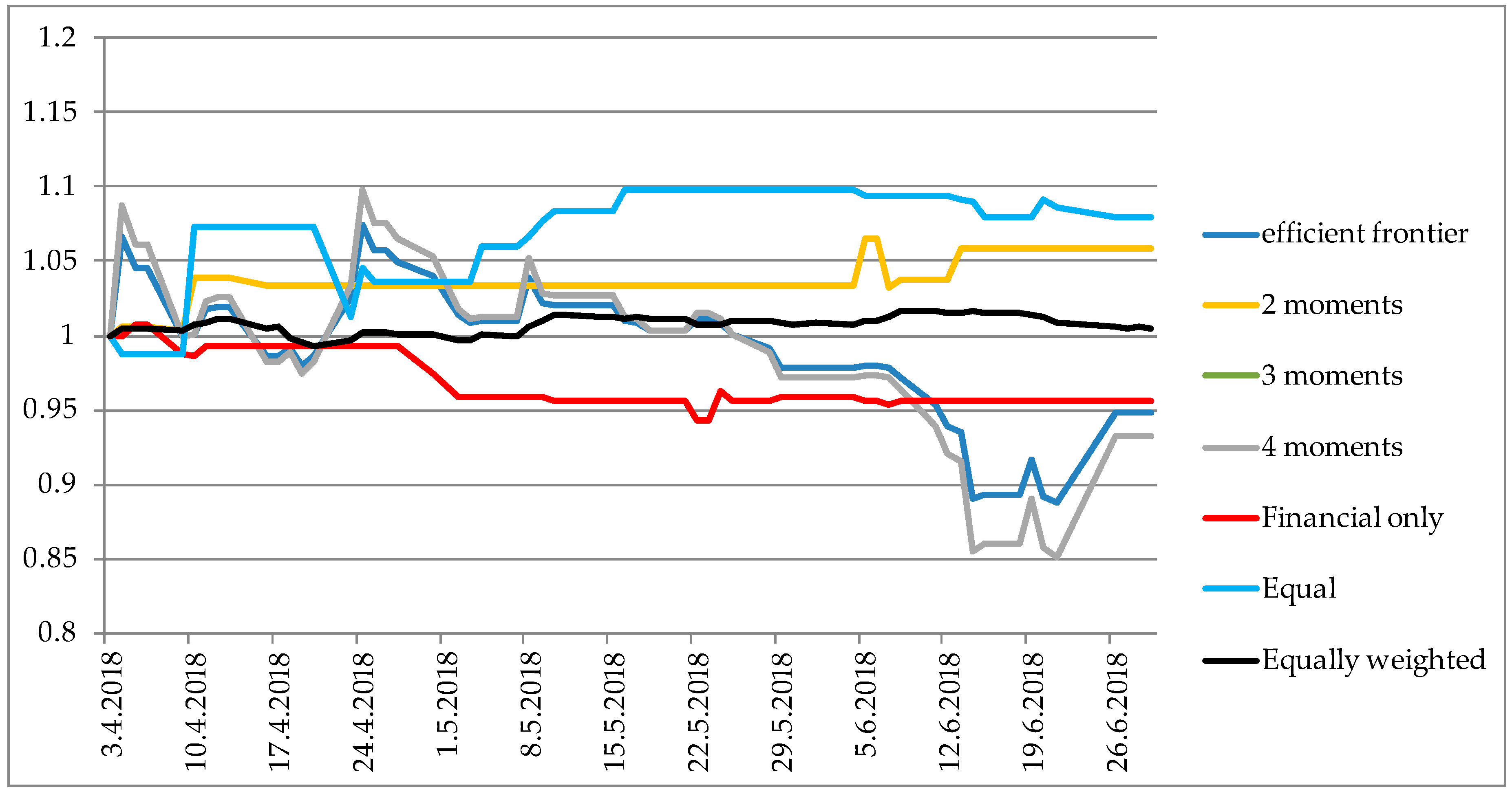
5. Backtesting Portfolio Results

Now we focus on the out of sample results by performing backtesting of the portfolios constituting the efficient frontiers on Figure 4 in order to evaluate the performance based upon ranking from the GRA approach. The performance measures are calculated based upon the Knight and Satchell (2002) performance measurement book. It is assumed that an investor uses the GRA ranking system results from Table A2 in order to construct portfolios at the beginning of 2018 and holds those portfolios until mid 2018. For every efficient frontier from Figure 4, we extracted 4 portfolios: minimum variance, maximum return and two in between to represent different risk aversions in the analysis. Thus, in total we observe 24 different portfolios and the equally weighted one as well. The characteristics of those portfolios are given in Table 3. It can be seen that regarding the realized return, the best portfolio in total was the one where equal weights were given to all of the criteria in the GRA ranking system with the return maximization approach. In general, the “2 moments” portfolios obtained the best results regarding the realized returns, due to having positive returns on for all of the selected portfolios. In terms of risk, the overall best performing were the “Financial only” criteria portfolios. However, investors observe these measures in combination and not separately. That is why firstly we compare Sharpe ratios for every portfolio in order to obtain reward to risk ratios. It can be seen that in general, the “2 moments” portfolios achieve greatest (positive) values of the Sharpe ratio, especially when investors aim to maximize the portfolio returns. The “3 moments” portfolios obtained the worst performance regarding this ratio out of sample. This is somewhat in line with Figure 4 where the “3 moments” frontier was the farthest from the original efficient frontier, while the “2 moments” frontier was the closest.
Finally, we calculated Certainty Equivalent (CE) values for every portfolio in the sample, by comparing in first two columns rankings based upon only the first two moments of each portfolio and in the last two columns by adding the skewness and kurtosis preferences into account as well. In that way, the rankings of the portfolios are based upon all of the portfolio moments, since we assumed that investor’s preferences depend upon first 4 moments. Although the “2 moments” portfolios had in general greater values of CEs for the first two moments, the last two columns indicate that the “3 moments” portfolios could be preferred over other ones. Although these portfolios had negative realized returns, in these scenarios the skewness and kurtosis had such preferable values that in the overall ranking of the portfolios, the rankings change. This is affected by investor’s preferences and aversions towards each portfolio moment (in these two last scenarios it is assumed that every moment is equally weighted in the utility function). Since the “3 moments” portfolios were not attractive based upon the return, risk and Sharpe ratio criteria, it could be said that these portfolios could be recommended to those investors who are more focused on higher moments of the portfolio rather than risks and returns (especially returns since they were negative for the majority of cases). By excluding the “3 moments” portfolios, again it can be seen that the “2 moments” portfolios exhibit the greatest CEs in majority cases.
Finally, the simulated values of each portfolio from the maximization5 scheme in Table 3 were depicted on Figure 5 in order to see which scenario could have been beneficial for the investor. The “equally weighted” and “2 moments” portfolios could have achieved greatest returns for the investor if he had structured his portfolio based upon the GRA analysis in 2017. There exists the potential to form the portfolio based upon the GRA ranking, since several portfolios achieved greater values compared to the value of the original efficient frontier portfolio.

6. Discussion

Based upon the results from the empirical analysis, several key points can be concluded. Firstly, both of the hypotheses can be confirmed. The first research question asked if GRA approach results can indicate a good portfolio structure. This was observed on Figure 3 and Figure 4 and how the GRA portfolios moved towards the original efficient frontier. The resulting portfolios moved closer to the efficient frontier in cases where return distribution moments were taken into consideration. This is in line with previous empirical and theoretical research on the importance of distribution moments when investors make their decisions. The second question asked if portfolios resulting from GRA approach are better in terms of risk and return compared to the benchmark of the equally weighted portfolio. This was confirmed when both figures were commented, where it can be seen that all of the GRA portfolios had greater returns for the same value of risk and had lower risk with the same level or portfolio return. Moreover, these two questions were further explored in the out of sample analysis where, based upon the results in 2017, we simulated 25 portfolio scenarios in order to obtain risks, returns and other measures (in Table 3). Next, the potential of this analysis can be seen in many different scenarios which can be simulated before making investment decisions. Here, we observed only about a dozen of different scenarios in which investors can observe how the characteristics of portfolios change by changing the structure of the portfolio based upon the GRA approach. Thus, future work can be extended upon developing reliable criteria and scenarios. Future work will extend this research as well by including partial moments of return distributions to see whether concepts from Post Modern Portfolio theory could result in better portfolio characteristics. Moreover, a dynamic analysis will be observed to see how factor changes over time influence portfolio selection and restructuring. Finally, different risk aversions will be included in the analysis as well, in order to obtain more insights into investor’s decision making based upon their risk aversion as well.

7. Conclusions

With many data available today on financial markets, many factors influence the decision making process when making investment decisions. Quantitative methods and models are constantly being developed in order to facilitate the portfolio and risk management process. The goal of this study was to investigate how results from GRA affect portfolio construction. The results were compared to the original efficient frontier constructed based upon Markowitz portfolio optimization.
Some of the pitfalls of the study were as follows. We observed only the full moments of return distributions and not partial moments (such as lower partial risk measures, etc.). Moreover, a static analysis was conducted due to observing the entire year 2017 characteristics of return distributions. In that way, it was possible to carry out the out of sample analysis only for the first half of 2018. However, a dynamic analysis could be provided only on a quarterly basis as well if all of the firms provide quarterly financial statements. The monthly or a weekly basis of the analysis could be possible only with market data. Some subjectivity is always present when making decisions based upon several criteria. This was the case in this study as well, when investor has to choose the weights on the factors in the GRA analysis, as well as when ranking the portfolios based upon their risk aversion, skewness preference and/or kurtosis aversion. We cannot discuss the usefulness of specific moments or financial ratios when ranking stocks, due to this being an empirical problem. This means that some factors used in the analysis can change over time and affect the ranking. In that way, dynamic analysis should be provided when applying this in practice. In this specific example, it is not advised to use financial ratios in the analysis, due to the efficient frontier being lower compared to other ones and being very short (i.e., small, providing less investment possibilities compared to other approaches).
Finally, since the results showed the potential of this methodology, there is hope that further applications will extend to achieving even better results in portfolio selection. However, the contribution of this research can be found in initial analysis of the GRA approach when making investment decisions.

Author Contributions

All authors contributed equally.

Funding

This research received no external funding. The APC was funded by institutions through the Knowledge Unlatched initiative and partially funded by MDPI.

Acknowledgments

The authors would like to thank three anonymous referees for their valuable comments and suggestions which contributed to the quality of the paper.

Conflicts of Interest

The authors declare no conflict of interest.

Appendix A

Table A1. Factors used in the analysis with corresponding desirable values.
Return Distribution:Market:Financial Ratios:
Expected return (ER) +
Standard deviation (SD) −
Coefficient of asymmetry (CA) +
Coefficient of skewness (CS) −
Trading volume (TV) −
Number of transactions (NT) −
Book to market ratio (BM) +
Price to earnings ratio (PE) +
Return on assets (ROA) +
Return on equity (ROE) +
Earnings per share (EPS) +
Total business efficiency ratio (TBR) +
Asset turnover ratio (ATR) +
Dividends per share (DPS) +
Source: authors.
Table A2. Stocks included in the analysis.
ADPL hADRS pADRS2 pARNT lATGR jATLN oATPL kAUHR j
BD62 bBLJE aCKML bDDJH pDLKV iERNT fHDEL iHHLD l
HMST lHT mHUPZ lIGH qINA dINGR pIPKK bJDGT k
JDPL kJMNC bJNAF kKOEI gKRAS bLEDO bLHRC lLKPC k
LKRI kLPLH kLRH lMAIS lMDKA jOPTE mPLAG lPODR b
PTKM eRIVP lRIZO fSAPN eSLRS lTHNK iTPNG kTUHO l
ULPL kULJN hVART cVIRO bVLEN hZB nZVZD b-
Source: ZSE (2018). Note: sector classification of the stocks is as follows: a—agriculture, forestry and fishery; b—food and tobacco production; c—production of textiles, clothing, leather and related products; d—manufacture of coke and refined petroleum products; e—manufacture of chemicals and chemical products; f—manufacture of computers and electronic and optical products; g—manufacture of electrical equipment; h—manufacture of transport equipment; i—construction; j—wholesale and retail trade; repair of motor vehicles and motorcycles; k—transport and storage; l—activities of providing accommodation and preparation and serving of food; m—telecommunications; n—financial and insurance activities; o—real estate business; p—legal, accounting, management, architectural and engineering engineering and technical testing and analysis; q—scientific research and development. Thus, in total 17 out of 23 sectors are included in the analysis.
Table A3. Ranking of stocks in the analysis.
Stock.p = 0.52 mom4 mom3 momOnly Financial0.7 mom; 0.3 otherRiskReturn
ADPL2467122691012
ADRS1821172635201334
ADRS23417101934141438
ARNT2622182524222432
ATGR2118131736152019
ATLN31491462185
ATPL38418406372
AUHR3335434338433049
BD623649475214464351
BLJE495352215525448
CKML1722953727226
DDJH5351485343494853
DLKV5232162932344023
ERNT3216211831252128
HDEL3946444850454541
HHLD4344374555393943
HMST1252031518116
HT458462017939
HUPZ4631554718543340
IGH4748495042505227
INA1415191525191716
INGR5139273733384622
IPKK3038393945363537
JDGT281146271944633
JDPL4147425144414747
JMNC275051349485121
JNAF8123341126417
KOEI11136132851211
KRAS1523142417131630
LEDO5555544954555555
LHRC9337213263
LKPC619151688714
LKRI42926287162710
LPLH5203423423813
LRH7951112438
MAIS1324122022112320
MDKA2252822212157
OPTE5437313649424242
PLAG101011916759
PODR1633223310212544
PTKM5052535448535052
RIVP4272103102218
RIZO3143404651403450
SAPN2334363827313124
SLRS2227413513352831
THNK4854505541514954
TPNG1930233139241945
TUHO11821114
ULPL2941244123283825
ULJN4045454452474429
VART2536303246303235
VIRO3542384247373646
VLEN4440324030334115
ZB3726253053292936
ZVZD20283512932531
Source: authors.

References

  1. Ang, Andrew, and Geert Bekaert. 2002. International Asset allocation With Regime Shifts. Review of Financial Studies 15: 1137–87. [Google Scholar] [CrossRef]
  2. Arditti, Fred, and Haim Levy. 1975. Portfolio efficiency analysis in three moments: The multiperiod case. The Journal of Finance 303: 797–809. [Google Scholar] [CrossRef]
  3. Arditti, Fred. 1967. Risk and the Required Return on Equity. The Journal of Finance 22: 19–36. [Google Scholar] [CrossRef]
  4. Athayde, Gustavo, and Renato Galvão Flôres. 1997. A CAPM with Higher Moments: Theory and Econometrics. Discussion Paper EPGE-FGV. Rio de Janeiro: EPGE/FGV. [Google Scholar]
  5. Banz, Rolf. 1981. The relationship between return and market value of common stocks. Journal of Financial Economics 9: 3–18. [Google Scholar] [CrossRef] [Green Version]
  6. Basu, Sanjoy. 1977. The Investment Performance of Common Stocks in Relation to their Price to Earnings Ratio: A Test of the Efficient Markets Hypothesis. The Journal of Finance 32: 663–82. [Google Scholar] [CrossRef]
  7. Briec, Walter, Kristiaan Kerstens, and Octave Jokung. 2006. Mean-variance-skewness portfolio performance gauging: A general shortage function and dual approach. Management Science 531: 135–49. [Google Scholar] [CrossRef]
  8. Campbell, John, and Robert Shiller. 1988. The dividend-price ratio and expectations of future dividends and discount factors. Review of Financial Studies 1: 195–228. [Google Scholar] [CrossRef]
  9. Campbell, John. 1987. Stock returns and the term structure. Journal of Financial Economics 18: 373–99. [Google Scholar] [CrossRef]
  10. Cremers, Jan-Hein, Mark Kritzman, and Sebastian Page. 2003. Portfolio Formation with Higher Moments and Plausible Utility. In Revere Street Working Paper Series in Financial Economics 272-12. Cambridge: State Street Associates. [Google Scholar]
  11. Chen, Hsing-Hung. 2008. Stock selection using data envelopment analysis. Industrial Management & Data Systems 108: 1255–68. [Google Scholar] [CrossRef]
  12. Chen, Kung, and Shimerda Thomas. 1981. An Empirical Analysis of Useful Financial Ratios. Financial Management 10: 51–60. [Google Scholar] [CrossRef]
  13. Datar, Vinay, Narayan Naik, and Robert Radcliffe. 1998. Liquidity and stock returns: An alternative test. Journal of Financial Markets 12: 203–19. [Google Scholar] [CrossRef]
  14. Deng, Ju-Long. 1982. Control problems of Grey Systems. Systems and Control Letters 5: 288–94. [Google Scholar] [CrossRef]
  15. Deng, Ju-Long. 1989. Introduction to Grey System Theory. The Journal of Grey Systems 1: 1–24. [Google Scholar]
  16. Dia, Mohamm. 2007. A Portfolio Selection Methodology Based on Data Envelopment Analysis. INFOR: Information Systems and Operational Research 47: 71–79. [Google Scholar] [CrossRef]
  17. Dimitropoulos, Panagiotis, and Dimitrios Asteriou. 2009. The Relationship between Earnings and Stock Returns: Empirical Evidence from the Greek Capital Market. International Journal of Economics and Finance 11: 40–50. [Google Scholar] [CrossRef]
  18. Edirisinghe, Nalin Chanaka, and Xin Zhang. 2007. Generalized DEA model of fundamental analysis and its application to portfolio optimization. Journal of Banking & Finance 31: 3311–35. [Google Scholar] [CrossRef]
  19. Fama, Eugene F., and Kenneth R. French. 1988. Dividend yields and expected stock returns. Journal of Financial Economics 22: 3–25. [Google Scholar] [CrossRef]
  20. Fama, Eugene F., and Kenneth R. French. 1992. The Cross-Section of Expected Stock Returns. The Journal of Finance 47: 427–65. [Google Scholar] [CrossRef]
  21. Fama, Eugene F., and Kenneth R. French. 1993. Common risk factors in the returns on stocks and bonds. Journal of Financial Economics 33: 3–56. [Google Scholar] [CrossRef]
  22. Fama, Eugene F., and Kenneth R. French. 1995. Size and Book-to-Market Factors in Earnings and Returns. The Journal of Finance 50: 131–55. [Google Scholar] [CrossRef]
  23. Fama, Eugene F., and Kenneth R. French. 1996. Multifactor Explanations of Asset Pricing Anomalies. The Journal of Finance 51: 55–84. [Google Scholar] [CrossRef] [Green Version]
  24. Fama, Eugene F., and William Schwert. 1977. Asset returns and inflation. Journal of Financial Economics 5: 115–46. [Google Scholar] [CrossRef]
  25. Gardijan, Margareta, and Tihana Škrinjarić. 2015. Estimating investor preferences towards portfolio return distribution in investment funds. Croatian Operational Research Review 62: 1–16. [Google Scholar] [CrossRef]
  26. Guidolin, Massimo, and Allan Timmermann. 2007. Asset allocation under multivariate regime switching. Journal of Economic Dynamics and Control 31: 3503–44. [Google Scholar] [CrossRef]
  27. Guidolin, Massimo, and Allan Timmermann. 2008. International Asset allocation under Regime Switching, Skew, and Kurtosis Preferences. The Review of Financial Studies 21: 889–935. [Google Scholar] [CrossRef]
  28. Huang, Kuang Yu, and Chuen-Jiuan Jane. 2008. An Automatic Stock Market Forecasting and Portfolio Selection Mechanism Based on VPRS, ARX and Grey System. Paper presented at IEEE Asia-Pacific Services Computing Conference, Yilan, Taiwan, December 9–12. [Google Scholar]
  29. Huang, Kuang Yu, Chuen-Jiuan Jane, and Ting-Cheng Chang. 2008. A RS Model for Stock Market Forecasting and Portfolio Selection Allied with Weight Clustering and Grey System Theories. Paper presented at IEEE Congress on Evolutionary Computation, CEC 2008, Hong Kong, China, June 1–6; pp. 1240–46. [Google Scholar] [CrossRef]
  30. Hur, Seok-Kyun, Chune Young Chung, and Chang Liu. 2018. Is Liquidity Risk Priced? Theory and Evidence. Sustainability 10: 1809. [Google Scholar] [CrossRef]
  31. Hur, Seok-Kyun, and Chune Young Chung. 2018. A novel measure of liquidity premium: Application to the Korean stock market. Applied Economics Letters 25: 211–15. [Google Scholar] [CrossRef]
  32. Hwang, Soosung, and Stephen Satchell. 1999. Modeling emerging market risk premia using higher moments. International Journal of Finance and Economics 44: 271–96. [Google Scholar] [CrossRef]
  33. Jane, Chuen-Jiuan, and Yu Kuang Huang. 2013. A Fusion Model for Stock selection Based on Decision Tree, Artificial Neural Network and Grey Relational Analysis. International Journal of Kansei Information 4: 115–22. [Google Scholar]
  34. Jondeau, Eric, and Michael Rockinger. 2006. Optimal portfolio allocation under higher moments. European Financial Management 121: 29–55. [Google Scholar] [CrossRef]
  35. Jurczenko, Emmanuel, and Bertrand Maillet. 2005. The Four-moment Capital Asset Pricing Model: Between Asset Pricing and Asset Allocation. In Multi-Moment Asset Allocation and Pricing Models. New York: John Wiley and Sons. [Google Scholar]
  36. Knight, John, and Stephen Satchell. 2002. Performance Measurement in Finance. Oxford: Elsevier Science Ltd. [Google Scholar]
  37. Korzeniewski, Jerzy. 2018. Efficient Stock Portfolio Construction by Means of Clustering. Folia Oeconomica 1: 85–92. [Google Scholar] [CrossRef]
  38. Kothari, Smitu P., and Jay Shanken. 1997. Book-to-market, dividend yield, and expected market returns: A time series analysis. Journal of Financial Economics 44: 169–203. [Google Scholar] [CrossRef]
  39. Kroll, Yoram, Haim Levy, and Harry Markowitz. 1984. Mean-Variance Versus Direct Utility Maximization. The Journal of Finance 39: 47–61. [Google Scholar] [CrossRef]
  40. Kuo, Yiyo, Taho Yang, and Guan-Wei Huang. 2008. The use of a grey-based Taguchi method for optimizing multi-response simulation problems. Engineering Optimization 40: 517–28. [Google Scholar] [CrossRef]
  41. Lewellen, Jonathan. 2004. Predicting returns with financial ratios. Journal of Financial Economics 742: 209–35. [Google Scholar] [CrossRef]
  42. Li, Hong-Yi, Chu Zhang, and Di Zhao. 2010. Stock Investment Value Analysis Model Based on AHP and Grey Relational Degree. Management Science and Engineering 4: 1–6. [Google Scholar]
  43. Liu, Sifeng, and Yi Lin. 2006. Grey Information Theory and Practical Applications. New York: Springer. [Google Scholar]
  44. Liu, Sifeng, and Yi Lin. 2010. Grey Systems, Theory and Applications. Berlin/Heidelberg: Springer. [Google Scholar]
  45. Liu, Sifeng, Yingjie Yang, and Jeffery Forrest. 2016. Grey Data Analysis: Methods, Models and Applications. Singapore: Springer Science + Business Media. [Google Scholar]
  46. Liu, Weimin. 2006. A liquidity-augmented capital asset pricing model. Journal of Financial Economics 823: 631–71. [Google Scholar] [CrossRef]
  47. Markowitz, Harry. 1952. Portfolio Selection. The Journal of Finance 7: 77–91. [Google Scholar] [CrossRef]
  48. Markowitz, Harry. 1959. Portfolio Selection: Efficient Diversification of Investments. New York: Wiley. [Google Scholar]
  49. Ministry of Finance. 2018. Available online: https://www.mfin.hr (accessed on 13 December 2018).
  50. Mohammadi Pour, Rahmatollah, Zhaleh Alavimoghadam, and Adel Fatemi. 2016. Comparison of Selected Performance of Portfolio Investment Companies by Using of Grey Forecasting and Johnson’s Index in Tehran Stock Exchange Market. Advances in Mathematical Finance & Applications 1: 15–28. [Google Scholar]
  51. Muhammad, Noor, and Frank Scrimgeour. 2014. Stock Returns and Fundamentals in the Australian Market. Asian Journal of Finance & Accounting 6: 271–90. [Google Scholar] [CrossRef]
  52. Müller, Sigrid, and Mark Machina. 1987. Moment preferences and polynomial utility. Economics Letters 23: 349–53. [Google Scholar] [CrossRef]
  53. Palepu, Krishna, and Paul Healy. 2010. Business Analysis & Valuation: Using Financial Statements, 4th ed. Nashville: South-Western College Pub. [Google Scholar]
  54. Pástor, Ľuboš, and Robert Stambaugh. 2003. Liquidity risk and expected stock returns. Journal of Political Economy 1113: 642–85. [Google Scholar] [CrossRef]
  55. Pulley, Lawrence. 1981. A General Mean-Variance Approximation to Expected Utility for Short Holding Periods. Journal of Financial and Quantitative Analysis 16: 361–73. [Google Scholar] [CrossRef]
  56. Reinganum, Marc. 1981. Misspecification of asset pricing: Empirical anomalies based on earnings yields and market values. Journal of Financial Economics 9: 19–46. [Google Scholar] [CrossRef]
  57. Salardini, Firoozeh. 2013. An AHP-GRA method for asset allocation: A case study of investment firms on Tehran Stock Exchange. Decision Science Letters 2: 275–80. [Google Scholar] [CrossRef]
  58. Shiller, Robert. 2005. Irrational Exuberance, 2nd ed. Princeton: Princeton University Press. [Google Scholar]
  59. Singh, Arjun, and Raymond Schmidgall. 2002. Analysis of financial ratios commonly used by US lodging financial executives. Journal of Retail & Leisure Property 2: 201–13. [Google Scholar] [CrossRef]
  60. Steuer, Ralph, Yue Qi, and Markus Hirschberger. 2008. Portfolio Selection in the Presence of Multiple Criteria. In Handbook of Financial Engineering. New York: Springer Science, pp. 3–24. [Google Scholar]
  61. Škrinjarić, Tihana. 2018a. Revisiting Herding Investment Behavior on the Zagreb Stock Exchange: A Quantile Regression Approach. Econometric Research in Finance 3: 119–62. [Google Scholar]
  62. Škrinjarić, Tihana. 2018b. Testing for Seasonal Affective Disorder on Selected CEE and SEE Stock Markets. Risks 6: 140. [Google Scholar] [CrossRef]
  63. Vidović, Jelena. 2013. Investigation of Stock Illiquidity on Central and South East European markets in Naive Portfolio Framework. Economic Thought and Practice 22: 537–50. [Google Scholar]
  64. Wei, Guiwu. 2011. Grey Relational Analysis Model for Dynamic Hybrid Multiple Attribute Decision Making. Knowledge-Based Systems 24: 672–79. [Google Scholar] [CrossRef]
  65. Wu, Liansheng. 2000. A Survey and An Analysis of Investor’s Demands for Listed Companies’ Accounting Information. Economic Research Journal 4: 41–48. [Google Scholar]
  66. ZSE. 2018. Available online: https://www.zse.hr (accessed on 1 November 2018).
1
Liquid in terms of number of transactions. Although research exists on how (il)liquidity affects stock returns, here we include more liquid stocks due to having more data to make calculations with. In 2017, in total 93 stocks were traded on ZSE. Problems with liquidity are not something new for ZSE. Namely, as Škrinjarić (2018a) states: in the period from September 2014 until May 2018, there were only 9 stocks which were traded at least 90% of the time, 17 with 75%, 25 with 60% and 37 with 30% of the whole period. The usual approach is to pick the liquid stocks which have been traded most frequently in a period. More details can be seen in Škrinjarić (2018b) or Vidović (2013).
2
Moreover, we do not choose to invest only in the best stock, due to diversification possibilities within Modern Portfolio Theory.
3
Sharpe ratio was calculated based upon the 91 day Treasury bill interest rate of the Ministry of Finance (2018) in Croatia which was equal to 0.36% in the observed period.
4
Values of 1 and 2 were chosen based upon Guidolin and Timmermann (2008) who used 2, 5 and 10; Ang and Bekaert (2002) where authors used 5 and 10. Guidolin and Timmermann (2007) showed that the results of ranking are robust if the coefficient is in the interval (0, 20]. Additionally, we calculated Certainty Equivalent for values 5 and 10 and the rankings remained the same. Quadratic utility function was chosen for the calculation of Certainty Equivalent due to results in Pulley (1981), Kroll et al. (1984) and Cremers et al. (2003) who compared the rankings of the quadratic utility function to other functional forms of investor’s utility and the results showed that the differences were nonsignificant.
5
Maximization of portfolio return problems were chosen since these portfolios could have enabled an investor to achieve the best results in terms of return series. Other 3 scenarios from Table 3 are omitted, but are available upon request; the portfolio values have similar relations one to another.
Figure 1. Grey relational grades for the analyzed stocks, different values of distinguishing coefficients.
Ijfs 07 00001 g001
Figure 2. Grey relational grades for the analyzed stocks, different criteria.
Ijfs 07 00001 g002
Figure 3. Comparison of efficient frontier with other frontiers, fixed weights of stocks in portfolios.
Ijfs 07 00001 g003
Figure 4. Comparison of efficient frontiers, optimization resulted weights.
Ijfs 07 00001 g004
Figure 5. Simulated portfolio values for the case of maximizing the return portfolio.
Ijfs 07 00001 g005
Table 1. Average, minimum and maximum values of factors for the whole sample.
FactorAverageMinMax
SD0.0200.0030.073
CS23.5703.194127.755
TV637,612.691800.0007,892,835.000
NT2914.218260.00016,276.000
ER0.000−0.0030.003
CA0.722−6.8479.195
BM2.9230.00178.930
PE5.121−30.87579.841
ROA0.428−2.23026.362
ROE−0.343−50.45368.125
EPS1584.2940.02845,894.157
TBR1.0470.2012.673
ATR7.9260.007208.657
DPS41.8310.0001649.937
SD—standard deviation; CS—coefficient of skewness; TV—trading volume; NT—number of transactions; ER—expected return; CA—coefficient of asymmetry; BM—book to market ratio; PE—price to earnings ratio; ROA—return on assets; ROE—return on equity; EPS—earnings per share; TBR—total business efficiency ratio; ATR—asset to earnings ratio and DPS—dividend per share. Source: authors.
Table 2. Grey relational grade for each stock, distinguishing coefficient value is 0.5.
Stockp = 0.5Stockp = 0.5
ADPL0.5303KRAS0.5418
ADRS0.5401LEDO0.4358
ADRS20.5213LHRC0.5535
ARNT0.5276LKPC0.569
ATGR0.5364LKRI0.5771
ATLN0.5886LPLH0.5746
ATPL0.518LRH0.5652
AUHR0.5224MAIS0.5454
BD620.5205MDKA0.5889
BLJE0.4855OPTE0.4592
CKML0.5406PLAG0.5526
DDJH0.461PODR0.5417
DLKV0.4702PTKM0.4829
ERNT0.5224RIVP0.511
HDEL0.5152RIZO0.5229
HHLD0.5104SAPN0.533
HMST0.5458SLRS0.5356
HT0.4984THNK0.4873
HUPZ0.4959TPNG0.5398
IGH0.4874TUHO0.6111
INA0.5435ULPL0.5248
INGR0.4778ULJN0.514
IPKK0.5242VART0.5281
JDGT0.5255VIRO0.521
JDPL0.5139VLEN0.5076
JMNC0.5269ZB0.5198
JNAF0.5537ZVZD0.5389
KOEI0.5477
Source: authors.
Table 3. Comparison of performances of simulated portfolios in 2018.
PortfolioRealized Return (%)Standard Deviation (%)Sharpe RatioCertainty Equivalent (CE)
123
mom
4
mom
Efficient frontierMin risk0.8270.4621.3990.0080.0080.3471.777
Portfolio 10.8270.4621.7880.0080.0080.3471.777
Portfolio 2−3.5673.455−1.032−0.036−0.037−0.679−0.880
Max return−5.1524.520−1.140−0.053−0.054−0.766−1.038
2 momentsMin risk0.9410.7971.1810.0090.0090.4421.724
Portfolio 11.3820.7131.9370.0140.014−0.0841.194
Portfolio 22.0240.7552.6810.0200.0200.1431.695
Max return5.9171.3884.262 *0.0590.059−0.194−1.081
3 momentsMin risk0.1970.5910.333−0.044−0.0440.0250.594
Portfolio 1−2.6601.067−2.493−0.018−0.0180.7141.778
Portfolio 2−1.7920.746−2.403−0.027−0.0270.747 *1.845 *
Max return−4.3671.817−2.403−0.002−0.0020.7211.819
4 momentsMin risk−0.2230.952−0.235−0.002−0.0020.304−0.178
Portfolio 12.7900.9512.9350.0280.028−0.927−1.336
Portfolio 2−0.5632.597−0.217−0.006−0.006−0.590−0.850
Max return−6.7785.960−1.137−0.070−0.071−0.784−1.057
Financial onlyMin risk0.3110.6150.506−0.044−0.044−0.850−1.353
Portfolio 10.1960.3830.5120.0020.002−0.851−1.352
Portfolio 20.1610.319 *0.5050.0020.002−0.848−1.343
Max return−4.3671.817−2.4030.0030.0030.7211.819
EqualMin risk−1.6770.812−2.065−0.017−0.017−1.395−2.722
Portfolio 11.3711.0171.3490.0140.014−1.456−2.713
Portfolio 23.8881.6842.3090.0390.039−0.751−1.010
Max return7.977 *3.0652.6020.079 *0.079 *0.2620.793
Equal weights
-0.4700.5930.7930.0050.005−0.4410.135
Note: greatest return, minimal risk, greatest Sharpe ratio3 and greatest Certainty Equivalent for each category of 4 portfolios is in bold and the values with asterisks are denoted as being best in respective rows. Numbers 1 and 2 denote the coefficient of absolute risk aversion for calculation of Certainty Equivalent with respect to the quadratic utility function4. 3 mom and 4 mom columns denote the Certainty Equivalent with respect to 3 and 4 moments based utility functions as in Jurczenko and Maillet (2005), where equal weights were added to all portfolio moments. Source: authors.

