1. Introduction
Modeling aggregate loss (
Duan 2018;
Frees 2014;
Meyers 2007;
Shi 2016) using insurance risk factors is a key aspect in the decision-making of rate change review application. In
Duan (
2018), a logistic regression model was proposed to classify the loss data of a Chinese company into different risk levels using the burden index. Multivariate negative binomial models for the insurance claim counts were proposed by
Shi (
2014) to capture the potential dependent structure among the different claim types. In
David (
2015), the Poisson regression and negative binomial models were applied to a French auto insurance portfolio to investigate the degree of risk using claim counts data. In
Najafabadi (
2017), a k-inflated negative binomial mixture regression model was proposed to model the frequency and severity of reported claims in an Iranian third-party insurance data set. Authors in
Tang (
2014) proposed a new risk factor selection approach based on EM algorithm and LASSO penalty, for a zero-inflated Poisson regression model. The analysis of car insurance data from the SAS Enterprise Miner database was then used to show the usefulness of the proposed method in rate-making. However, all those works focused on the study of the loss experience of an individual company, rather than on the total loss at the industry level. In auto insurance regulation, approval of the submitted rate change application by insurance companies requires significant statistical evidence from a company’s past loss experience
Chen (
2009). Thus, a study of total loss behavior at the industry level becomes important in providing a constructive review of a company’s rate change applications.
Auto insurance companies often consider various risk factors based on the available loss experience, such as age, number of years of license, gender, number of years without accidents, territory, and vehicle rate group. In addition, various socio-demographic factors are used to differentiate the risk levels of drivers. More recently, usage-based insurance (UBI) programs have been offered by many major insurance companies. The analysis of data associated with UBI (e.g., mileages, traffic conditions, and driving habits) are new types of rating factors (
Cripe 2012;
Husnjak 2015;
Ma 2018). However, this is not the case for insurance regulators because the detailed individual loss information is not available for the review of a rate change. Of course, insurance regulators are not interested in reproducing company results when reviewing the rate change application, but they need an analysis based on the aggregated loss experience from major insurance companies or the whole industry. A review decision made by a regulator must be supported by key findings on the rating factors at the industry level. Since insurance companies use many risk factors in pricing, the question arises as to whether one can focus only on the major rating factors in the review process. Answering to this question calls for use of suitable predictive modeling techniques that can be applied in rate filings review, particularly in classification of risk (
Hamid 2011;
Watson 2004). The aim of such modeling techniques is to find better understanding of the characteristics of major risk factors. In Canada, among many other risk factors, Class and Driving Record (DR) are the most important factors. The DR is a factor that includes levels 0, 1, 2, …6+, where each level represents the accumulated non-accident years of an insured, while Class represents a combination of driver age, gender, and use of vehicle. The information that is used for carrying out relativity estimates is either loss cost or loss ratios. None of the current predictive modeling of insurance loss uses industry aggregate loss data, and focus on major risk factors. This motivated us to investigate if major risk factors are able to capture most of the variation of total loss data at an industry level.
In predictive modeling, to better capture the major variation of loss data, considerable effort has been spent on finding the optimal solution in terms of the minimum overall bias (
Zhao 2011;
David 2015;
Frees 2015;
Garrido 2016). Due to its significant impact on insurance rate regulation, loss cost or loss ratios modeling became popular (
Harrington 1992;
Tennyson 2009). When loss cost is used, the bias is defined as the difference between the predicted loss cost and its actual observed value. The minimum overall bias considers both the bias of estimating pure premium for each class of insured and its associated number of exposures. To estimate the risk relativities, minimum bias procedure (MBP) introduced by
Bailey (
1963) has often been used, and it has become a traditional approach in non-life insurance pricing (
Feldblum 2003). Recent research on actuarial practice has demonstrated that generalized linear models (GLMs), an advanced statistical method, have become prevalent in the field of rate-making, risk modeling, or forecasting in most of the European and Asian countries (
Ohlsson 2010). In
Zhao (
2011), GLM was used to model the loss frequency and loss severity of automobile insurance in China to analyze the impacts of automobile, human, and rating territory on loss frequency and severity. In
David (
2015), an overview of GLM in the calculation of the pure premium given the observable characteristics of the policyholders was presented. In
Garrido (
2016), GLM was fitted to the marginal frequency and the conditional severity components of the total claim cost with the introduction of dependence between the number of claims and the average claim size was studied. The main reason for the prevalence of GLM is that it enables a simultaneous modeling of all possible risk factors as well as determination of the retention of risk factors in the model.
In the risk classification system of auto insurance companies, rate-making is one of the most important aspects among many others, such as underwriting and marketing strategies (
Outreville 1990). Its major goal is to develop a set of risk factor relativities that can be further used for pricing an insurance policy. Also, rate-making that uses industry-level data is a typical task in a rate filings review. Even though an insurance company has access to the transactional loss and claim data, it is clear that the rate-making process is based on the aggregate level of the company data. This is because it is not in the company’s interest to evaluate the risk of a single exposure. The rate-making is done based on the average loss costs of each combination of the levels of risk factors. The average loss cost (or simply the loss cost in the following discussion) is defined as the total loss divided by the total exposures within each possible combination of the levels of risk factors, where the total loss and the total exposures are the aggregate measures of loss and exposures for that particular combination. Traditionally, within actuarial practice, the estimates of rating factor relativities are conducted by using MBP (
Feldblum 2003). In rate filings reviews, often the rating variables of Class and DR are considered. The relativities are estimated by MBP separately for each data set, that is, from each respective combination of different years, territories, and coverages. The problem with this approach as a rate-making technique is that the potential interactions among rating variables are not considered. Thus, the results may not be comparable. Also, MBP is a numerical approach that is unable to statistically evaluate the difference between relativities.
In this paper, we present the results of a comparative study employing MBP and GLM as modeling tools. We focus on the study of industry-level data used in rate filings reviews to decide if major data variation could be retained in the models, and how it is affected by the risk factors under consideration. We investigate the consistency of the results obtained from both MBP and GLM methods. It is expected that one could replicate the results obtained by MBP by applying GLM to the same data set. For ease of understanding the interaction of rating variables, we mainly focus on the predictive modeling of loss cost using DR, Class, and accident year as the major rating variables. The significance of this work is in providing general guidelines for the use of predictive modeling in an insurance rate filings review for auto insurance regulators. In particular, this work demonstrates the usefulness of GLM in rate-making for rate filing purposes. This approach can help us to understand how a decision is being made when focusing only on major risk factors. This paper is organized as follows. In
Section 2, we summarize the data used in this work, and discuss the methodologies, including MBP and GLM, used for producing the results presented in this paper. In
Section 3, comparative results obtained from MBP and GLM under different model settings are analyzed. Finally, in
Section 4, we conclude our findings and provide summary remarks.
2. Methods
2.1. Minimum Bias Procedure
Let
be a collection of observed values. It can be loss severity, claim counts, average loss cost, or loss ratio, depending on the interest of modeling, and how we define a response variable. Let
be the value contributed by the
ith DR level (i.e., DR takes values 0, 1, 2, 3, 4, 5, 6+), and let
be the value contributed by the
jth level of Class. Also, let
be the number of exposures of risk in the (
i,
j)th combination of levels of the underlying risk factors. The objective of MBP is to find optimal solutions for
and
, subject to the following two sets of equations as constraints (
Feldblum 2003):
Numerically, MBP iteratively solves for
and
using the following two equations, until
and
converge at the
lth step, where
The relativities are obtained by selecting kth levels as a base, which are defined as , for DR, and , for Class.
2.2. Generalized Linear Models for Rate-Making
The main idea of generalized linear models (GLMs) (
De Jong 2001;
Haberman 1996;
Ohlsson 2010) in rate-making is to model a transformation of the expected value of a response variable, which in our case is
. The transformation function
is called the link function, where
. The model that is used to explain the transformation function
g is a linear model, and it can be written as follows:
where
=
and
=
. Here,
and
are dummy variables. That is,
takes the value 1 when
i corresponds to the
ith level of DR, otherwise it is zero.
takes the value 1 when
j corresponds to the
jth level of Class, otherwise it is zero.
is the error random variable assumed to have a certain probability distribution function.
is referred to as a systematic component. The variance of
is assumed to have the following functional relationship with the mean response:
where
is called a variance function. The parameter
scales the variance function
, and
is a constant assigning a weight. This result comes from a family of distributions called the exponential family (
McCullagh 1989), which determines the parameters
and
. The case when
implies a normal distribution. If
, then the distribution is Poisson. If
, then it is a gamma distribution, and if
, then it is an inverse Gaussian distribution (
Mildenhall 1999). These distributions are the distributions used in this work. In general, the following relationship between variance function and mean value of response is considered:
We discussed the cases when
p=0, 1, 2, and 3. For
or
, the distributions are called Tweedie distributions (note that the inverse Gaussian belongs to this class of distribution) (
Dunn 2001;
Tweedie 1957).
In the case when
g is an identity function, GLM becomes a general linear model. Thus, the relativities are obtained by computing the exponential transformation of model coefficients, which are denoted by
and
,
and
j (
Ohlsson 2010). In this work, the following model specifications are investigated:
Systematic component: ∼;
Error distribution functions: Gaussian, Poisson, inverse Gaussian, and gamma;
The multiplicative model, resulting in a log link function for GLM, that, is ;
The number of exposures is used as a weight value.
From the way the systematic component for the given data is modeled, one can see that for each combination of risk factor levels, the loss cost has a unique distribution, and the model specifies a common variation captured by the error distribution function. Because the standard deviation estimate is available for each level of risk factors, one can easily construct their confidence intervals based on the normal approximation approach. To validate the choice of log-scale, a Box-Cox transform (
Osborne 2010) can be applied. If the obtained parameter value is close to zero, this implies that a selection of the log link function is appropriate for the given data.
2.3. Handling Weights in GLM
In general, it is expected that GLM will be applied to either an industry-level data summary or a company’s transactional data summary. There are no fundamental differences between these two cases, as they are only subject to different levels of data aggregation. In transactional data summary, the loss costs are calculated in exactly the same way as in the industry data summary. It is important to consider a suitable weight function for each cell data, so that the variance function of the pre-defined error distribution in GLM is appropriately modeled. The number of exposures associated with each cell of the two-way data summary (by DR and Class) is used as a weight for the loss cost approach. The main purpose is to offset the different levels of data variation among the cells. Under the definition of the weight function in GLM, the assumption of having an identical error distribution for each cell of loss cost becomes reasonable.
In practice, there is flexibility in specifying the weight function, but this depends on how each cell data within the summary is defined. In addition to the use of the number of exposures at each combination as a weight, a new type of weight function can be defined by
where
is the one-way summary of the number of exposures for the
ith level of DR, and
is the one-way summary of the number of exposures for the
jth level of Class.
is the total number of exposures. Also, another weight function can be defined by
when one wants to emphasize the importance of DR, by ignoring the effect of the number of exposures from the Class. Similarly, a third weight function can be defined by
2.4. Inclusion of Year as a Major Risk Factor
The estimates of relativities obtained from multiple-year loss experience are often considered to be more robust. One approach is to combine the multiple-year data together and ignore their year labels. In this case, the credibility of loss cost for each combination is improved as the corresponding number of exposures is increased with the increase of number of years of data. Thus, the number of exposures is now based on multiple years of aggregation. However, the disadvantage of this approach is that the effect from different years on relativity estimates is transferred to the relativities of other risk factors. A better approach is to add
as a major risk factor to the GLM, in which the systematic component is re-defined as
Since we added as another variable, = and =, where is a dummy variable taking the value 1 when k corresponds to the kth level of . The is the associated coefficient. In this approach, the effect from the factor can be estimated. Also, the data variation captured by the model is improved by the consideration of an additional risk factor. Under this approach, the estimate of relativity is less dependent on the choice of an error distribution function. This implies the robustness of estimating relativity using GLM. The relativity of reflects the level of loss cost for that particular year. Since loss costs of later years have not yet fully developed to the ultimate loss level, a smaller value of relativity of may only mean a lower loss cost for that particular year, based on the available reported loss amounts.
2.5. Fundamental Difference between MBP and GLM
The use of loss cost as a response variable is a common approach when applying MBP to industry-level data (
Brown 1988;
Garrido 2016;
Ismail 2009). The loss cost approach considers both the relativities caused by loss frequency and loss severity. Within the loss cost approach, the relativities are obtained by a conditional iterative process, which implies that the
lth step of the output of the algorithm becomes the input of the (
l+1)th step,
Brown (
1988). The minimization of the total bias is based on the marginal balance principle that is applied to each column and each row of the loss cost data matrix, respectively, where the row and the column correspond to DR and Class. Essentially, MBP treats the bias within each cell of the data matrix as being independently and identically distributed, without actually measuring its distribution. This method is less practical when the total number of risk factors is large, due to the nature of the numerical approach. This approach does not give optimal estimate for base rate (
Brown 1988), which is important for calculating pure premium. In terms of numerical convergence, the initial value condition plays an important role. The initial values are assigned based on the one-way summary of loss costs. Due to the nature of the iterative process, the final solution is often affected by the choice of initial values. Each value will be adjusted based on the result from the previous step.
Unlike MBP, GLM specifies an error distribution function for the bias of loss costs, and transforms observed values by link function to improve the linearity between the transformed response variable and the risk factors. The transformation is introduced to model a potential non-linear relationship via an appropriate mapping from the original space of the mean value of observations to a linear feature space. The selected error distribution function mainly captures the true distribution of underlying loss cost. Instead of placing a balance constraint for each row and column of data, GLM uses the assumption that within each row and each column, the error function is common to the bias. This constraint has a similar effect on determining a unique solution, as it was observed in MBP. However, in MBP, an iterative process is used to solve a non-linear optimization problem. The idea of using the GLM method is to fit the bias to a certain distribution and use a statistical approach to estimate the distribution parameters. In this case, an interval estimate of relativity becomes possible. Because of this, the use of GLM is more powerful than using MBP in terms of the statistical validation of test data. When specifying an equivalent constraint for both MBP and GLM, one can recover the same estimates of relativities from both MBP and GLM (
Brown 1988;
Mildenhall 1999).
With regards to making a prediction of loss costs, both MBP and GLM require a common base rate for all rating variables. The common base estimated using GLM corresponds to the intercept of the model. For MBP, it is calculated from the total loss divided by the total exposures for all risk factors. Therefore, the performances of MBP and GLM differ in minimizing overall bias: the base rate from GLM is a model estimate, but the base rate for MBP is just an empirical estimate. However, the estimated relativities can be the same for certain cases for both methods.
2.6. Some Discussions
In general, the use of GLM enables us to select variables according to their statistical significance. This is likely why GLM has been considered to be the most powerful tool for non-life insurance pricing (
Ohlsson 2010). One of the important tasks of the pricing problem is ensuring that risk factors and their levels are included in the model. As the dimension of the risk factors and their associated number of levels increase, it becomes challenging to interpret the impact of particular combinations of the rating variables on the loss cost. Therefore, focusing on the most significant rating variables may be superior. However, we do not encounter this difficulty within the scope of this work, as we only consider a few important risk factors that appear in the rate filings review. The relativities estimates of major risk factors become a general guideline for rate filings reviewers to better understand the nature of insurance rate fluctuations when comparing the results from different companies. Thus, the selection of a proper approach makes rate regulation statistically more sound, as the results are less affected by reviewer experience and judgement.
Recently, the generalized additive model (GAM) has been proposed in predictive modeling for rate-making (
Denuit 2004;
Fuzi 2016;
Klein 2014). From a technical perspective, GAM is an extension of GLM. In statistics, data are categorized into two types, numerical or categorical. When modeling data in practice, there is often no clear-cut rule about the data type. In most cases, it depends on expert opinion and the purpose of modeling. This means that for some of the variables within rate-making, we can have different types of treatments. For instance, the DR takes values 0, 1, 2, 3, 4, 5, 6+. If our goal is to estimate the average differential for each driving record, we assume that the collected data are categorical. However, since there is a natural ordering of the data, we expect that with the increase of the value of driving record, the differential decreases. It is reasonable to expect that there is a monotonic relationship within different driving records. Therefore, one can impose this relationship on a model by specifying the functional form of the Driving Record. This is the idea behind the extension of GLM to GAM.
3. Results
In this study, we considered an industry-level data set for accident years from 2007–2009, with third party liability (TPL) coverage and urban territory. The relativities of DR and Class at various levels were obtained for the accident year 2007 data set by both MBP and GLM. Additionally, a data set comprising these three accident years as a whole was used for relativity estimation for both cases of with and without
as a rating factor. The modeling and analysis were based on the aggregate measure of each combination of levels among all factors that we considered. The summary of average loss costs is reported in
Table 1. The value of each cell represents the loss cost of each given combination of levels from DR and Class. Notice that in the table the NA values mean that the loss costs were not available for these cells, which causes the problem of dealing with the missing values in the later computation. In some cases, zero values of the loss cost appeared in the summary data table. If this happens, then zero values were simply replaced by NAs. Ideally, we expected to have full information in the summary data table. Since we used industry-level data, the impact of missing values on some combinations of DR and Class was reduced when compared to the cases that dealt with company-level data. Thus, it makes sense to use the estimated relativities as a benchmark in rate filings review.
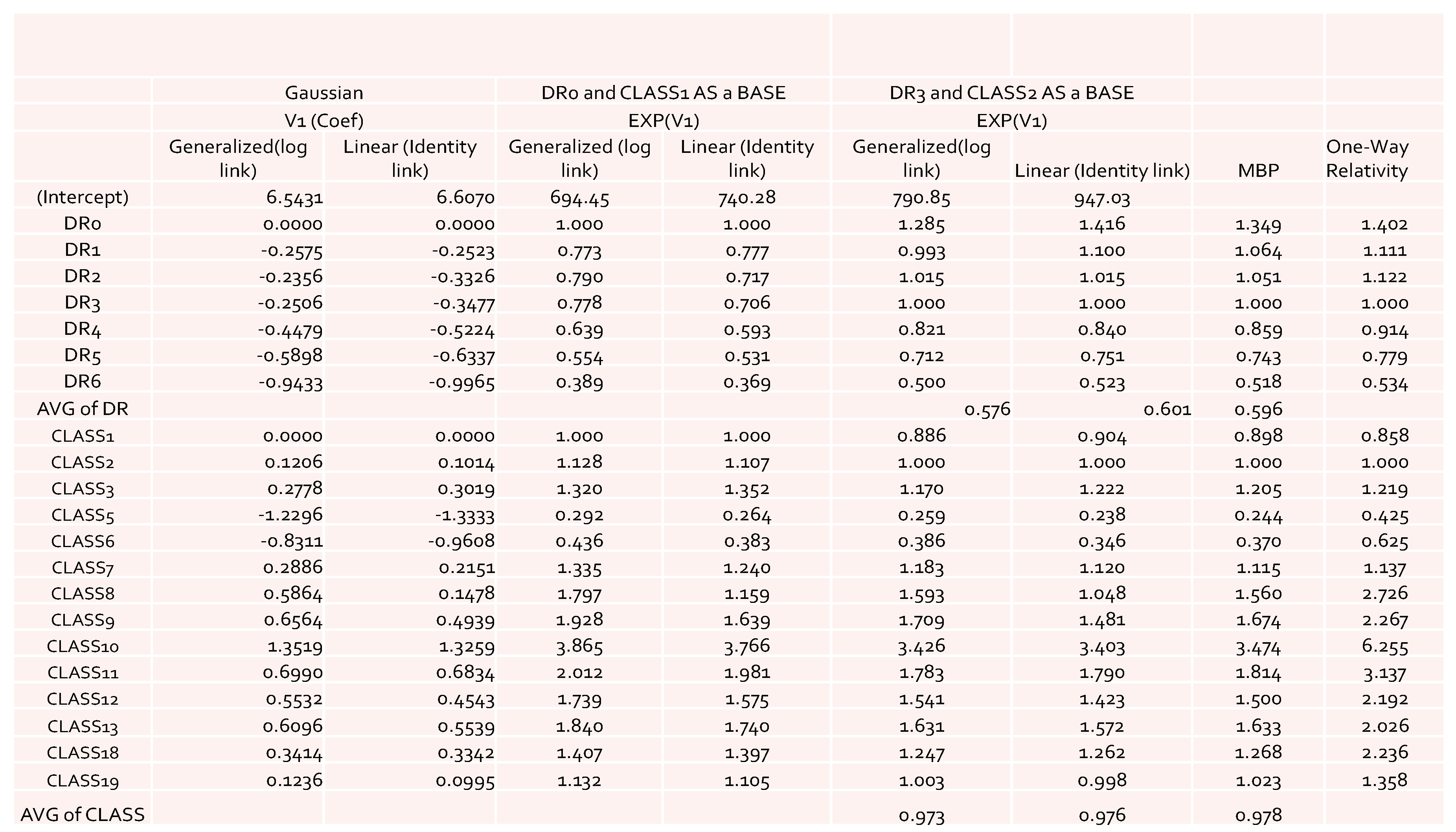
The obtained results of model coefficients and relativities are presented in
Figure 1 for the case of using Gaussian distribution as an error function. The results include both the results of the general linear model and of the generalized linear models. From
Figure 1, we can see that there were no significant large differences among the estimates of relativities. However, the general linear model gave slightly higher overall average relativities, which implies that the pure premium using results from the general linear model would be overestimated when compared to the generalized linear models. When GLM results were compared to the ones from MBP, a similar pattern was observed. This confirms our expectation that GLM would perform better in terms of reducing the effects of the interaction of risk factors, leading to lower estimates of relativities. However, this is only applicable for a Gaussian error function, which implies that the underlying assumption of the loss cost has to have a lighter tail distribution. This suggests that in modeling loss cost using GLM with a Gaussian error function, a large loss, corresponding to catastrophic events, must be removed before fitting the models to the data. This is because the loss data without removing large loss often follow a heavy-tailed distribution (
Bradley 2003;
McNeil 1997).
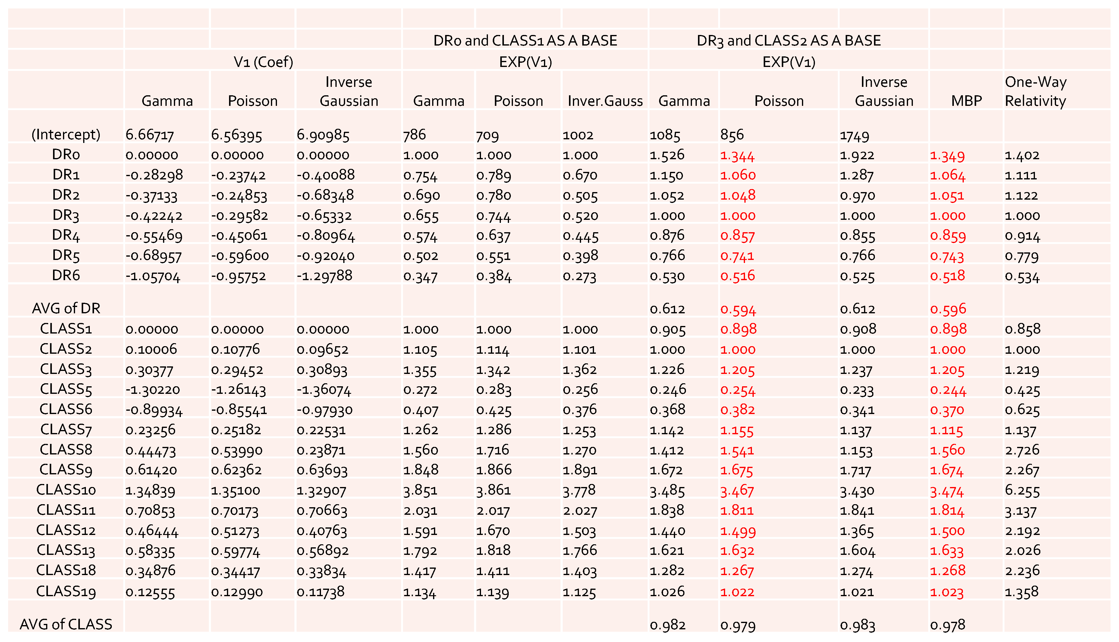
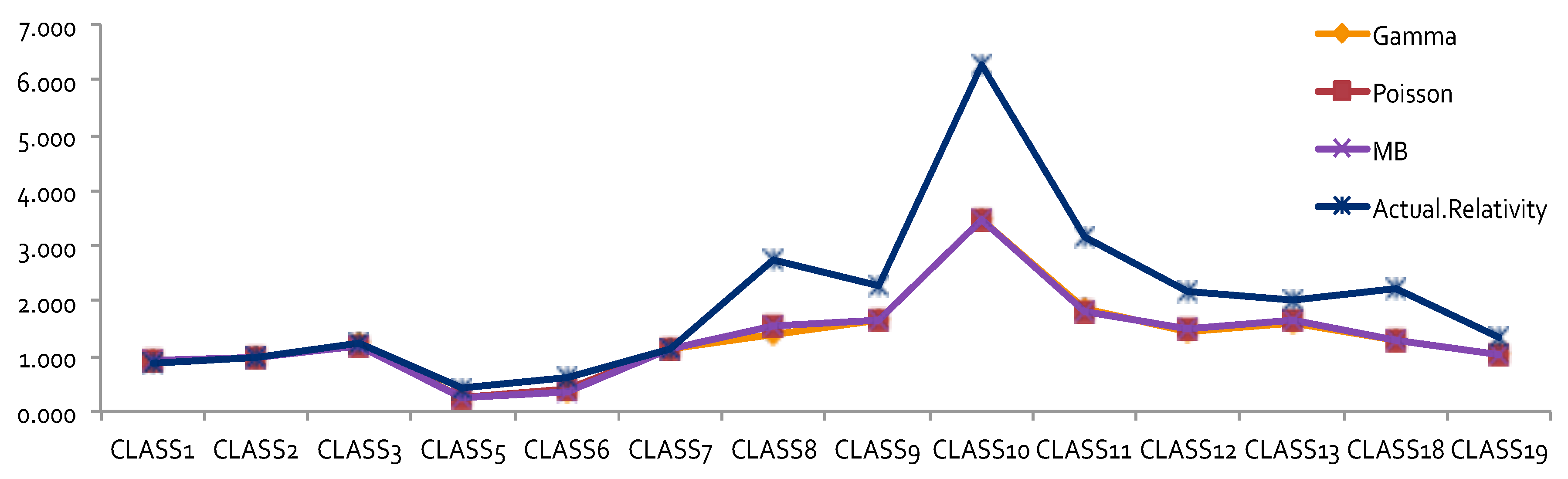
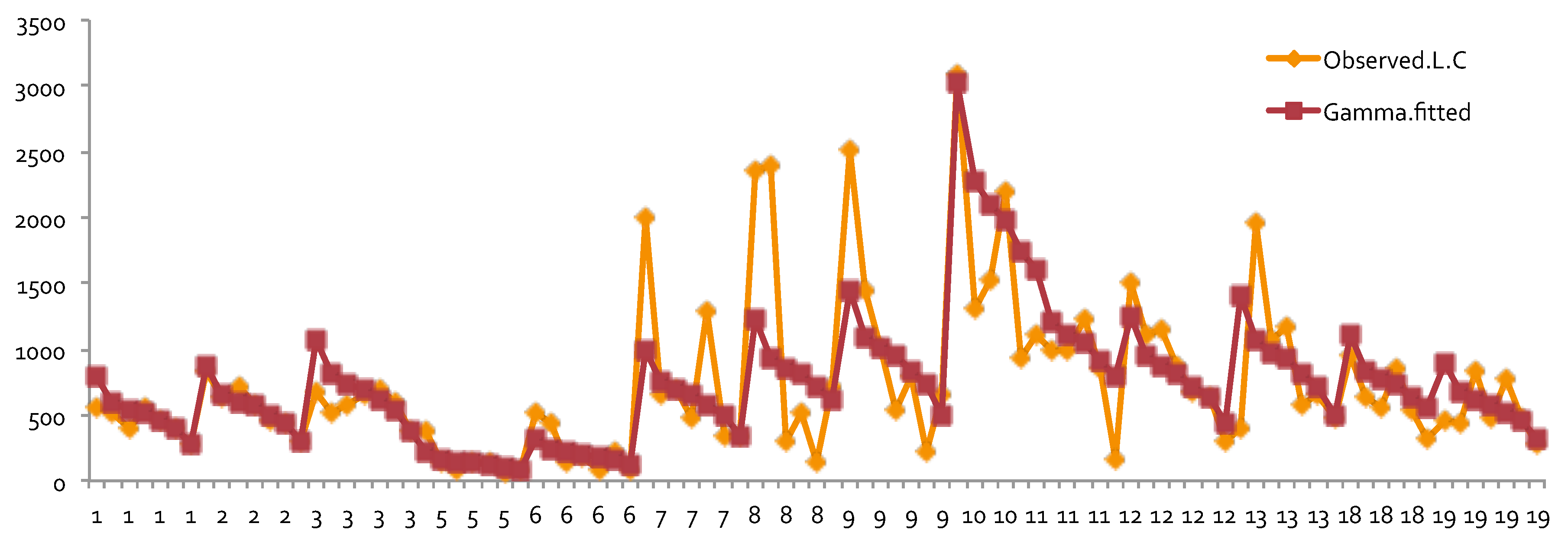
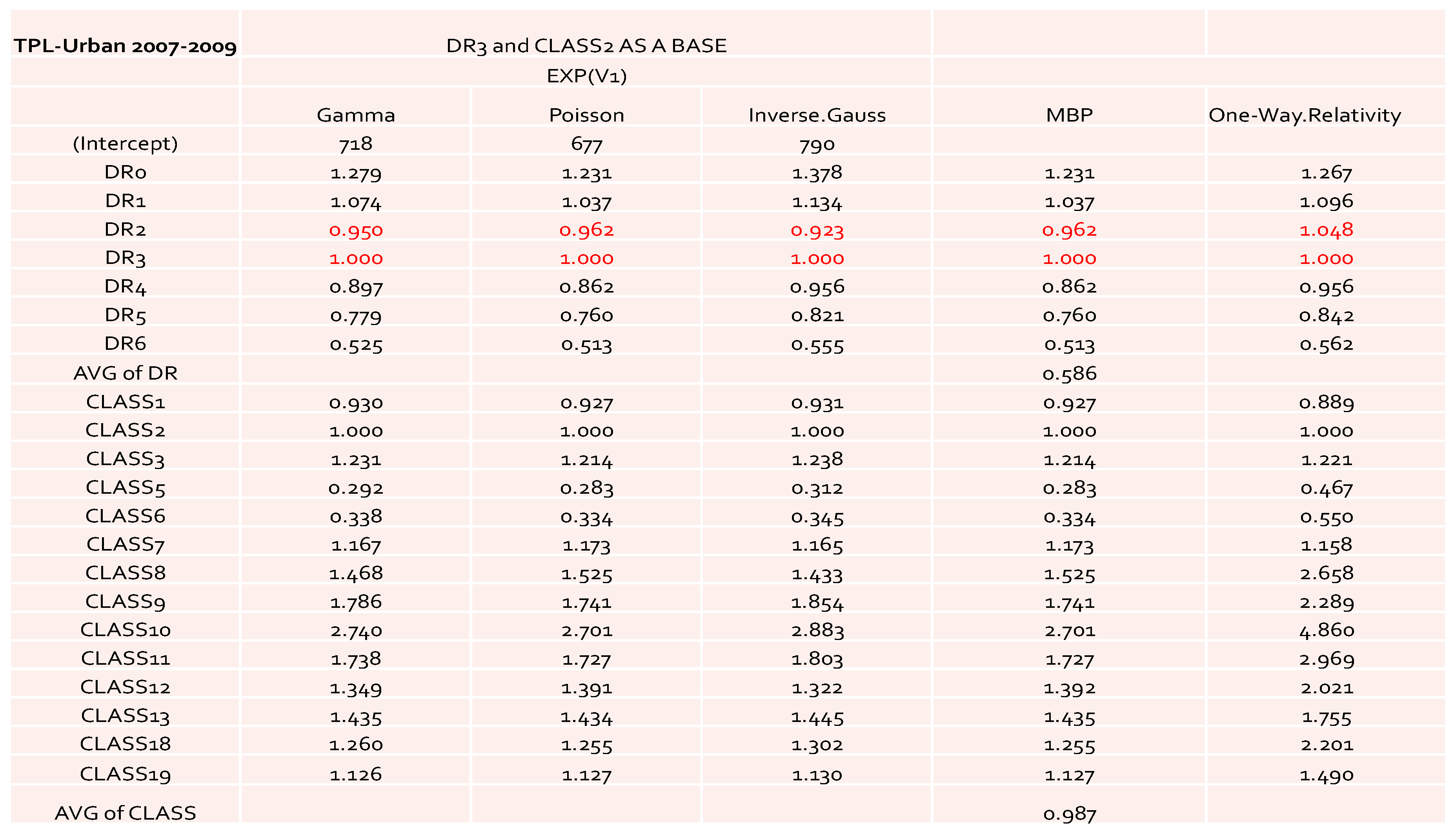
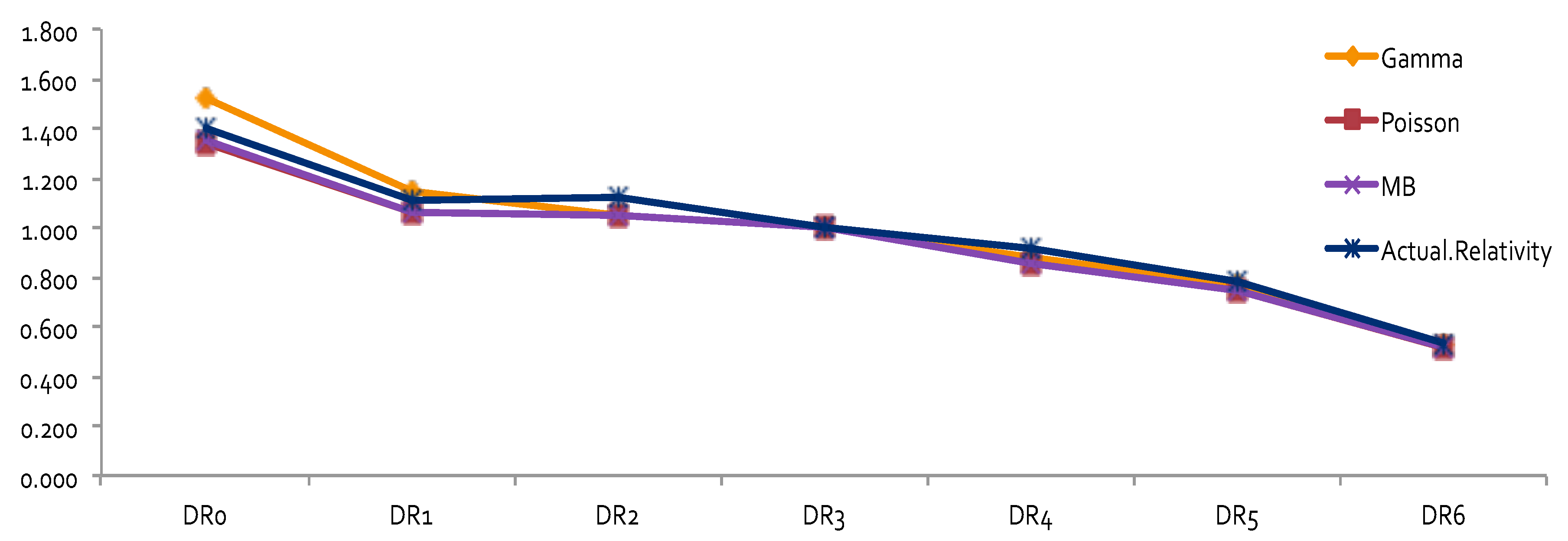
The results obtained by using other error distributions, including gamma and inverse Gaussian, are presented in
Figure 2. The estimates of relativities for both DR and Class were larger than the ones obtained from MBP or Poisson distribution. The MBP and Poisson distribution led to the same theoretical results—see
Brown (
1988). This may mean that the use of a heavy tail distribution in an error distribution function gives larger estimates of relativities. Risk increased when the tail of the loss distribution was heavier, resulting in larger relativities for the rating factors. When the relativities obtained from GLM or MBP were compared to one-way relativities, we saw that they were mostly underestimated. This suggests that more risk factors may need to be included in order to better capture data variation. Rate filings reviews do not aim at pricing, but focus instead on producing results that help to better understand the nature of major risk factors used by companies.
By looking at the loss cost or the one-way relativities of loss cost for DR1 and DR2 (i.e., the last column in both
Figure 1 and
Figure 2), we realized that there was a reversal for the relativity of DR1 and DR2. We expected a higher relativity for the insured who had less experience. Unfortunately, the results from the one-way summary were not as good as the ones obtained by GLM or MBP because the one-way relativity based on a two-way summary loss cost ignores the differences of the number of exposures among cells. Therefore, in order to better model loss costs using GLM, a suitable choice of a weight function needs to be specified, reflecting the difference of data value in each cell caused by the different levels of loss aggregation.
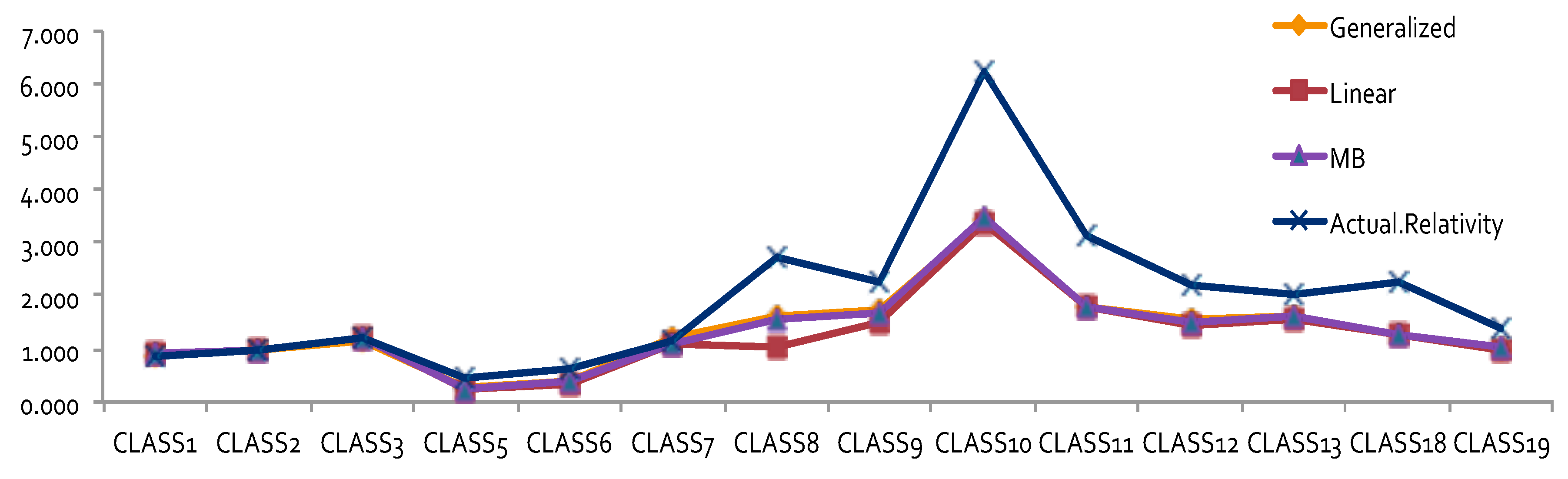
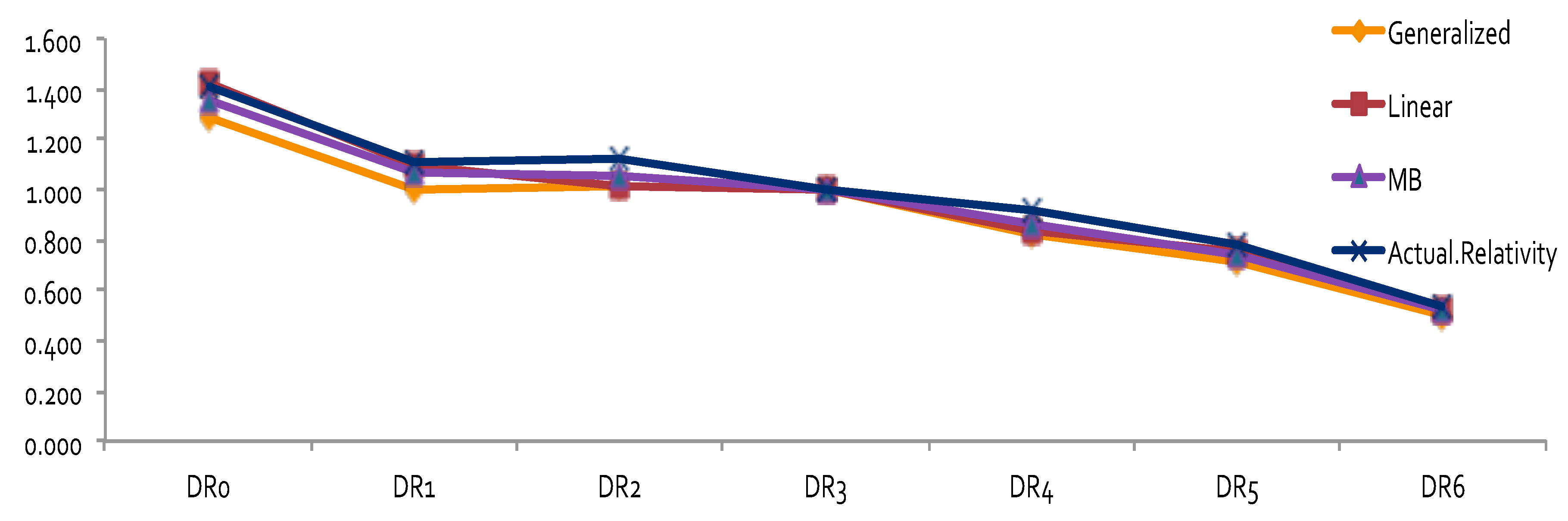
The results of relativity estimates and their comparisons under different model assumptions are reported in
Figure 3,
Figure 4,
Figure 5 and
Figure 6. In
Figure 3 and
Figure 4, the overall pattern for DR was consistent for all cases. Relativity decreased with the increase of the number of non-accident years. This means that prior driving record proved to have validity in predicting a driver’s accident risk. This result coincides with the results of in
Peck (
1983), who demonstrated the significant predictive power of DR as a rating factor. In all cases, the relativities of DR obtained from GLM were close to the actual relativities calculated from the one-way summary. For Classes 1 to 7, which contained the majority of the risk exposures, the estimated relativities for all considered models were close to the actual one-way estimates. The model estimates’ departure from the actual one-way relativities became significant only for those Classes that contained a smaller number of risk exposures. The values of the coefficients and relativities of the considered methods are displayed in
Figure 7. Overall, these values coincided with the actual values, but GLM underestimated the relativities at some levels of Class—namely, Class8, Class10, Class11, and Class18. We believe that this is due to both the missing values and the level of credibility of data from those classes. Combining Class with DR, we were able to see that Class was successful in explaining the loss cost data. A similar research outcome was reported in
Lourens (
1999). Unlike a single class with multiple characteristics as in our work, drivers’ sex, age, and level of education were used in
Lourens (
1999).
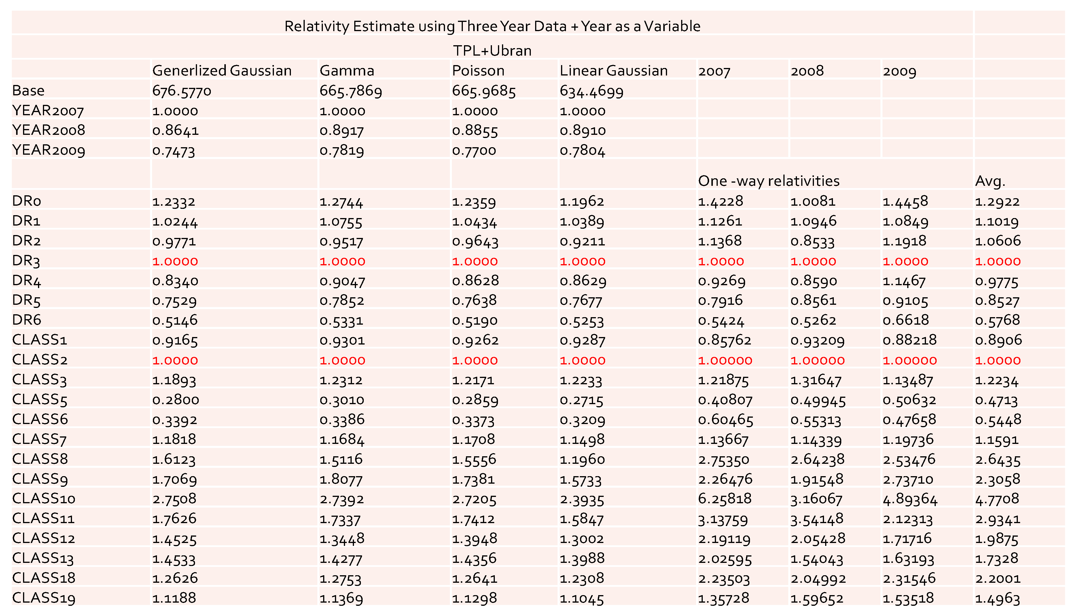
The values of the coefficients and relativities obtained by the GLM for the data with three accident years combined are reported in
Figure 8 and
Figure 9. Recall that for the one-way relativities we observed the reversal of the values for DR1 and DR2 in both the 2007 and 2009 accident years (see
Figure 1 and
Figure 2). However, after combining three years’ data, this reversal of the values disappeared in one-way relativities. This implies that the use of the data of three accident years combined was better in terms of discovering the desired pattern. The results obtained by GLM for both cases with and without
as a risk factor did not display a reversal phenomenon. Also, with the inclusion of
as a risk factor, we could capture its effect on loss cost. From the results of
Figure 8 and
Figure 9 we see that this effect was significant among different years.
From the results displayed in
Figure 8 and
Figure 9, we can conclude that the model with
as a risk factor was a good choice from the rate filings review prospective, as it could avoid extra uncertainty from single-year data. The results from the data of three years combined were more reliable and more suitable for acting as a benchmark for the rate filings review. The model can be easily extended to further include the territory as additional risk factor. However, we feel that from the rate filing review perspective it is not necessary, because it will significantly decrease the number of exposures for each combination of given levels. Also, we found that the definition of territory presents another difficulty, as it may change from time to time. Definitions of DR and Class are relatively more stable.
4. Conclusions
The GLM procedure with Poisson error distribution function is equivalent to MBP in estimating relativities. However, due to the different methods of estimating base rate, the GLM with Poisson error function outperformed MBP in terms of the overall bias. For the data considered, the gamma error function was the most appropriate error distribution. For the relativity estimation under multiple-year loss experiences, the gamma error distribution function was the only loss function that led to a monotonic decrease with the increase of driving experience. Because a monotonic decrease is desired for DR in auto insurance pricing, this suggests that the gamma error distribution function should be used. When GLM is applied to aggregate data, a weight function is needed if one believes that there is some bias from estimating average loss cost for each combination of risk factors, or if the level of data variation at each cell needs to be considered. The commonly used weight function is the number of exposures for each combination of the levels of the risk factors. However, GLM is able to reduce the effect of potential interaction of risk factors. Because of this, the obtained relativities for major risk factors are usually lower than those from the one-way analysis. GLM can be expanded by including additional rating variables, conducting a statistical test of significance, and evaluating the predictive power of the model. Since GLM is an efficient and reliable predictive tool, it is popular in other areas of predictive modeling.
The overall implication of the presented findings is that the pricing issues in a complex insurance system from the rate filings perspective is better understood. The estimates of major risk factors captured major pricing patterns. The results explain the natural variation in the process when reviewing a company’s rate change application. This enhances decision-making in operations using only major risk factors. because it is less affected by the details of the company’s results. Understanding how advanced statistical techniques work may also lead to a better communication with insurance companies in the process of discussing rate changes. Our study demonstrated that GLM is suitable as a predictive modeling technique in auto insurance rate filings review. The GLM relativities of major risk factors within rate filings review can be used as the benchmark for the same risk factors used in auto insurance pricing.


