A Continuous-Time Inequality Measure Applied to Financial Risk: The Case of the European Union


Abstract
1. Introduction
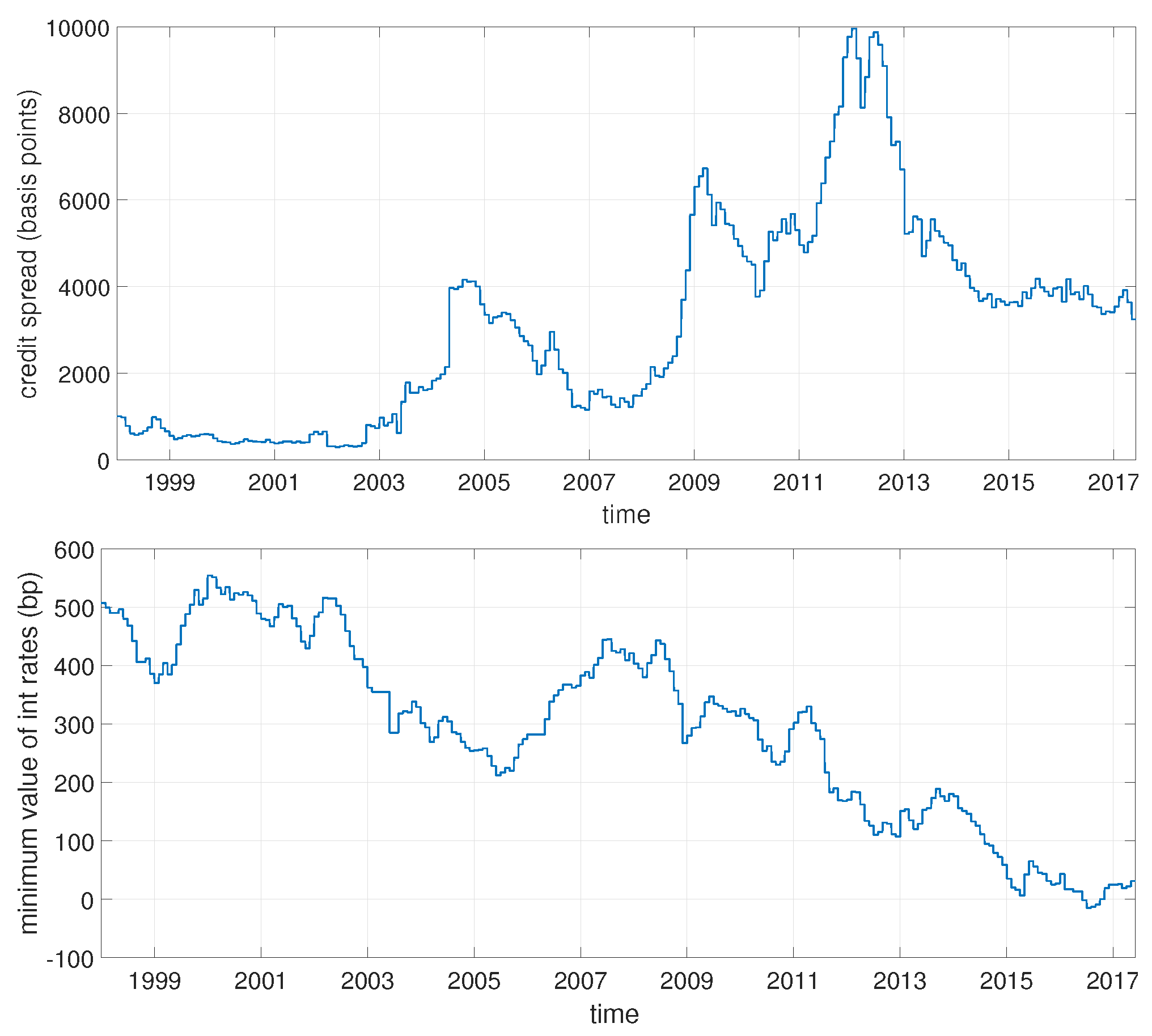
2. Data
3. Methodology
3.1. The Model for Rating Migrations
- , if ,
- .
3.2. Dynamic Measurement of the Inequality
3.3. Monte Carlo Simulation to Forecast the Financial Inequality
3.4. Estimation of the Infinitesimal Generator
4. Results and Discussion
4.1. Generator Matrix
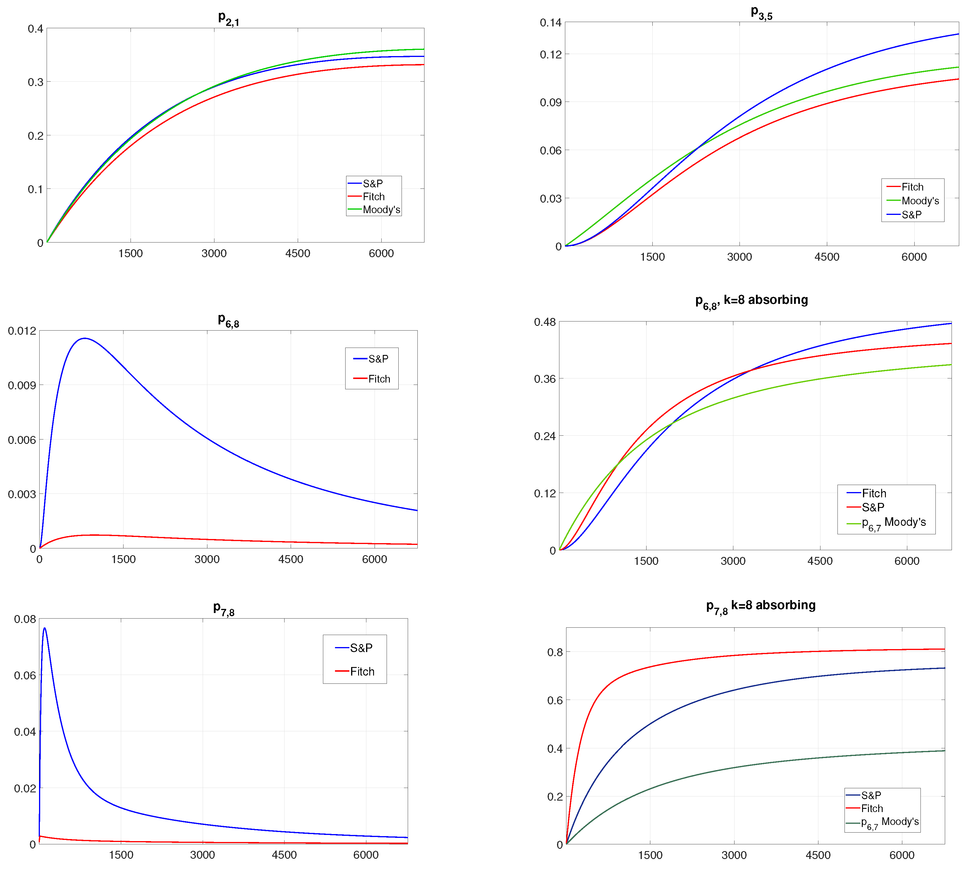
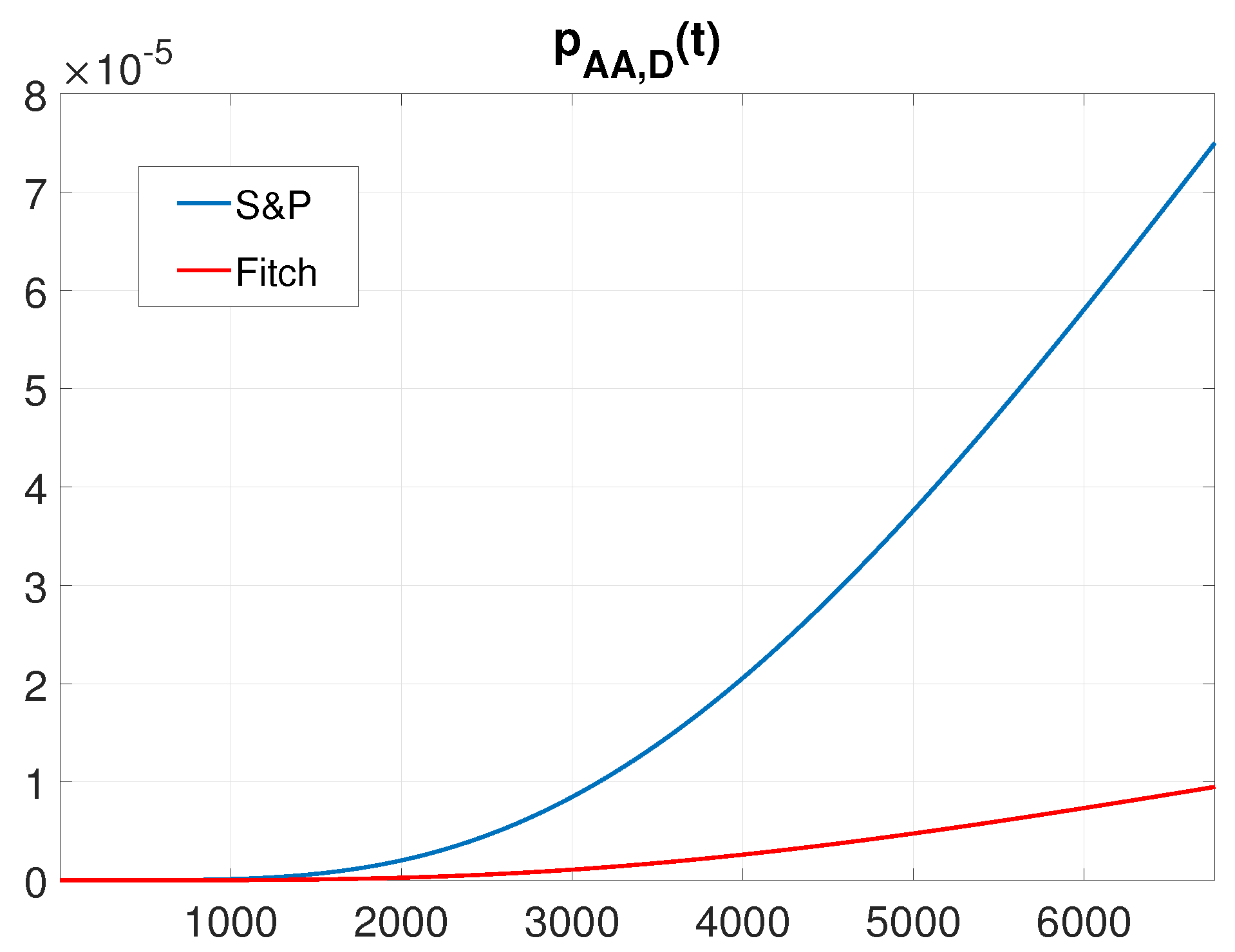
4.2. Rate of Occurence of Failures
- and fo Fitch and S&P and for Moody’s;
- and for Fitch and S&P and for Moody’s.
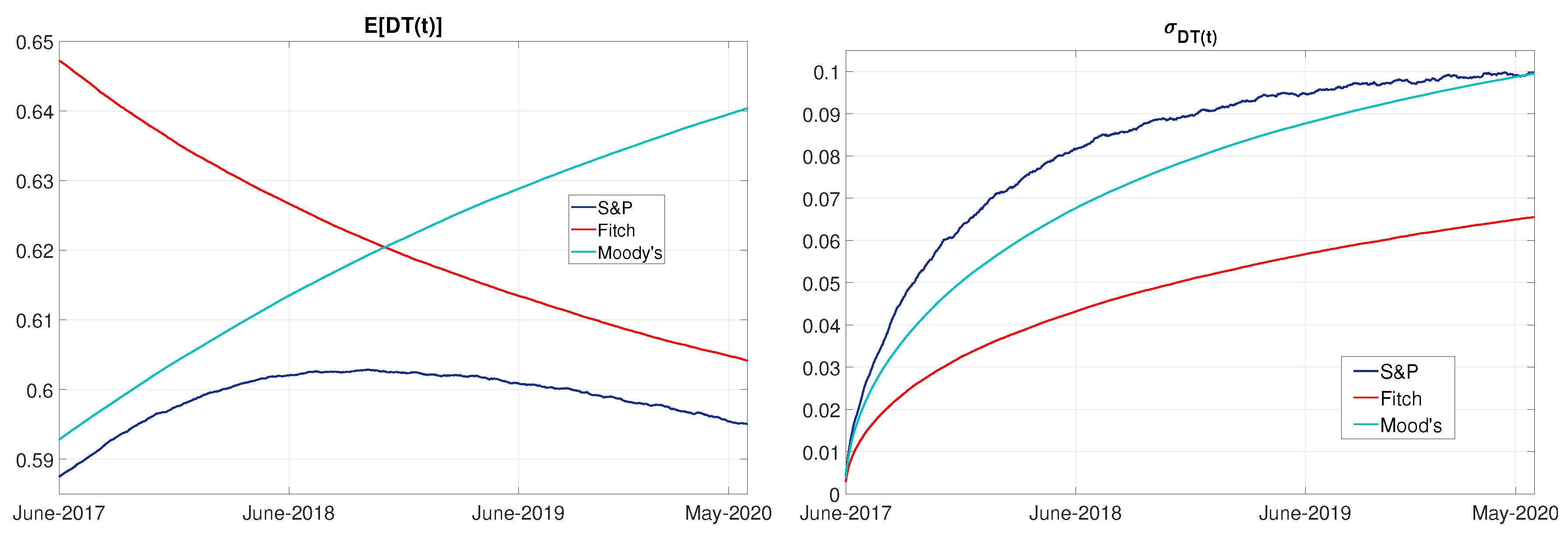
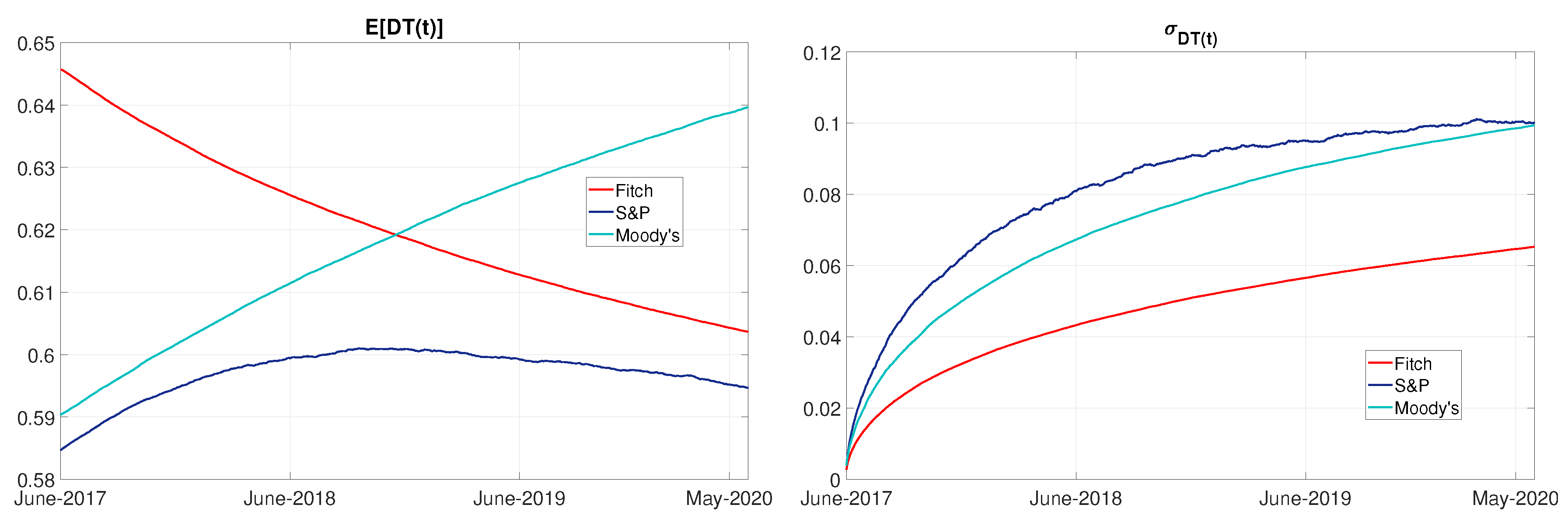
4.3. Financial Inequality
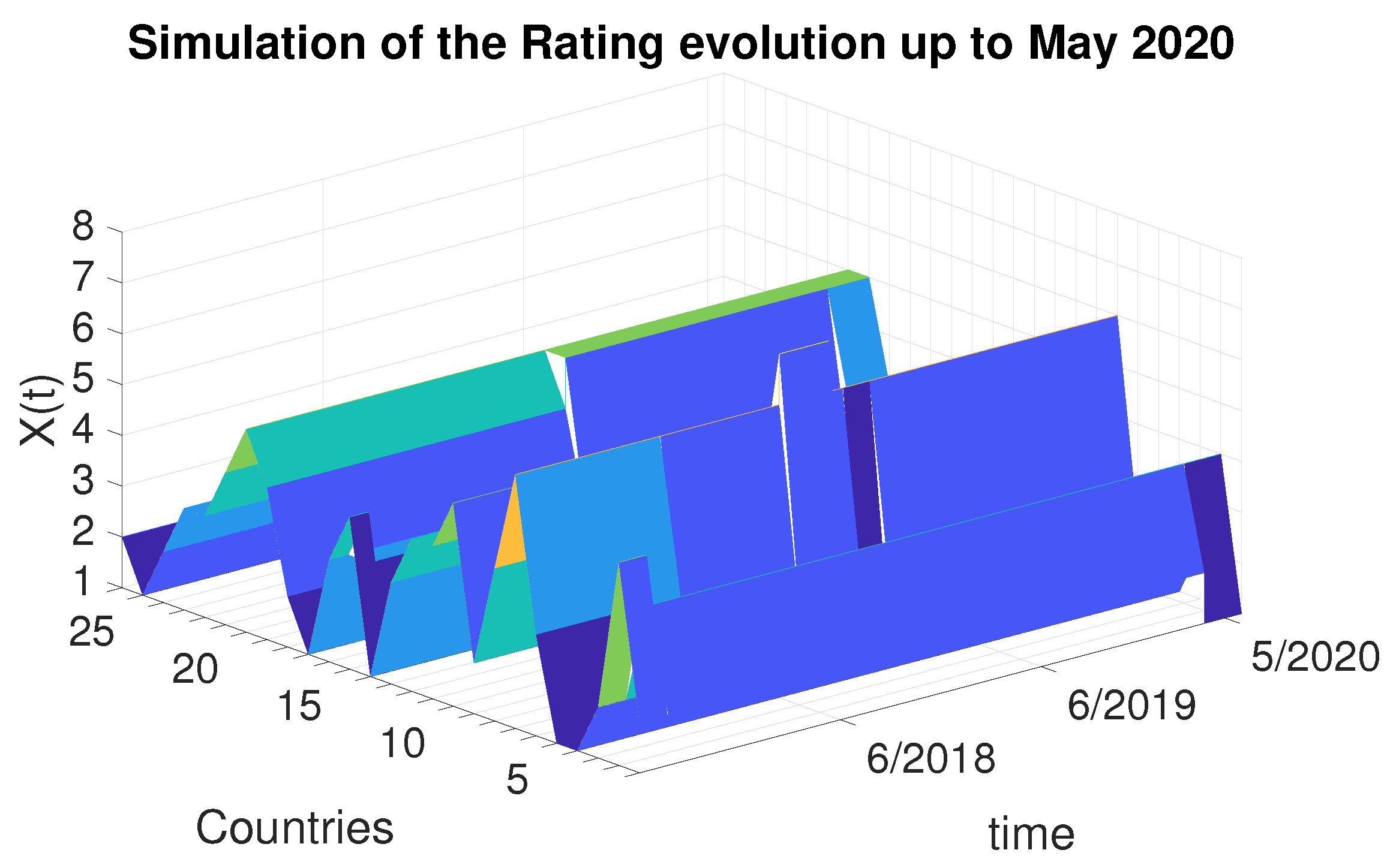
4.4. Simulation in the Case of Brexit
4.5. Discrete vs. Continuous
5. Conclusions
Author Contributions
Funding
Acknowledgments
Conflicts of Interest
References
- Albarran, Irene, Mercedes Ayuso, Montserrat Guillén, and Malena Monteverde. 2005. A multple state model for disability using the decomposition of death probabilities and cross-sectional data. Communications in Statistics: Theory and Methods 34: 2063–75. [Google Scholar] [CrossRef]
- Ausloos, Marcel, and Roy Cerqueti. 2016. Studies on Regional Wealth Inequalities: The Case of Italy. Acta Physica Polonica A 129: 959–64. [Google Scholar] [CrossRef]
- Bangia, Anil, Francis X. Diebold, André Kronimus, Christian Schagen, and Til Schuermann. 2002. Rating migration and he business cycle with application to credit portfolio stress testing. Journal of Banking & Finance 26: 445–74. [Google Scholar]
- Carty, Lea V., and Jerome S. Fons. 1994. Measuring changes in corporate credit quality. The Journal of Fixed Income 4: 27–41. [Google Scholar] [CrossRef]
- Cerqueti, Roy, and Marcel Ausloos. 2015. Statistical assessment of Regional wealth inequalities. Quality & Quantity 4: 2307–23. [Google Scholar]
- Christensen, Jens HE, Ernst Hansen, and David Lando. 2004. Confidence sets for continuous-time rating transition probabilities. Journal of Banking & Finance 28: 2575–602. [Google Scholar]
- Cowell, Frank. 2001. Measuring Inequality. Oxford: Oxford University Press. ISBN 9780199594030. [Google Scholar]
- D’Amico, Guglielmo. 2015. Rate of Occurence of Failures (ROCOF) of Higher-Order for Markov Processes: Analysis, Inference and Apllication to Financial Credit Ratings. Methodology and Computing in Applied Probability 17: 929–49. [Google Scholar] [CrossRef]
- D’Amico, Guglielmo, Giuseppe Di Biase, Jacques Janssen, and Raimondo Manca. 2017. Semi-Markov Migration Model for Credit Risk. London and Hoboken: Wiley-ISTE. [Google Scholar]
- D’Amico, Guglielmo, Giuseppe Di Biase, and Raimondo Manca. 2014. Decomposition of the population Dynamic Theil’s Entropy and its application to four European Countries. Hitotsubashi Journal of Economic 55: 229–39. [Google Scholar]
- D’Amico, Guglielmo, Giuseppe Di Biase, and Raimondo Manca. 2012. Income inequality dynamic measurement of Markov models: Application to some European countries. Economic Modelling 29: 1598–602. [Google Scholar] [CrossRef]
- D’Amico, Guglielmo, Jacques Janssen, and Raimondo Manca. 2005. Homogeneous semi-Markov reliability models for credit risk management. Decisions in Economics and Finance 28: 79–93. [Google Scholar] [CrossRef]
- D’Amico, Guglielmo, Jacques Janssen, and Raimondo Manca. 2011. A non-homogeneous Semi-Markov reward model for the credit spread computation. International Journal of theoretical and Applied Finance 14: 221–38. [Google Scholar] [CrossRef]
- D’Amico, Guglielmo, Stefania Scocchera, and Loriano Storchi. 2018. Financial risk distribution in European Union. Physica A 505: 252–67. [Google Scholar] [CrossRef]
- Dubois, Paul F., Konrad Hinsen, and James Hugunin. 1996. Numerical Python. Computational Physics 10: 262–67. [Google Scholar] [CrossRef]
- Ding-hua, Shi. 1985. A new method for calculating the mean failure numbers of a repairable system during (0,t]. Acta Mathematicae Applicatae Sinica 8: 101–10. [Google Scholar]
- Escalera, Morgan, and Wayne Tarrant. 2014. Sovereign Adaptive Risk Modelling and Implications for the Eurozone GREXIT Case. International Journal of Financial Studies 6: 4. [Google Scholar]
- Gavalas, Dimitris, and Theodore Syriopoulos. 2014. Bank credit risk management and Rating migration analysis on the business cycle. International Journal of Financial Studies 2: 122–42. [Google Scholar] [CrossRef]
- Hill, Paula, Robert Brooks, and Robert Faff. 2010. Variations in sovereign credit quality assessments across rating agencies. Journal of Banking & Finance 34: 1327–43. [Google Scholar]
- Huang, Jing-Zhi, and Ming Huang. 2012. How much of the corporate-treasury yield spread is due to credit risk? The Review of Asset Pricing Studies 2: 153–202. [Google Scholar] [CrossRef]
- Hunter, John D. 2007. Matplotlib: A 2D graphics environment. Computing in Science & Engineering 9: 90–95. [Google Scholar]
- Jarrow, Robert A., David Lando, and Stuart M. Turnbull. 1997. A Markov Model for the Term Structure of Credit Risk Spreads. The Review of Financial Studies 10: 481–523. [Google Scholar] [CrossRef]
- Jones, Eric, Travis Oliphant, and Pearu Peterson. 2001. SciPy: Open source scientific tools for Phyton. Available online: http: //www.scipy.org/ (accessed on 8 May 2017).
- Knieling, Jorg, and Frank Othengrafen. 2015. The economic and financial crisis: Origins and consequences. In Cities in Crisis: Socio-Spatial Impact of the Economic Crisis in Southern European Cities. London and New York: Routledge, pp. 13–26. [Google Scholar]
- Lando, David, and Torben M. Skødeberg. 2002. Analyzing rating transitions and rating drift with continuous observations. Journal of Banking & Finance 26: 423–44. [Google Scholar]
- McClean, S. 1980. A Semi-Markov Model for a Multigrade Population with Poisson Recruitment. Journal of Applied Probability 17: 846–52. [Google Scholar] [CrossRef]
- Nguyen, Nguyet. 2018. Hidden Markov Model for Stock Trading. International Journal of Financial Studies 6: 36. [Google Scholar] [CrossRef]
- Oliphant, Travis E. 2006. Guide to NumPy. Pravo: Brigham Young University. [Google Scholar]
- Papadopoulou, Aleka A., and Panagiotis C.G. Vassiliou. 1999. Continuous Time Non Homogeneous Semi-Markov Systems. In Semi-Markov Models and Applications. Edited by Jacques Janssen and Nikolaos Limnios. Boston: Springer. [Google Scholar]
- Sadek, Amr, and Nikolaos Limnios. 2005. Nonparametric estimation of reliability and survival function for continuous-time finite Markov processes. Journal of Statistical Planning and Inference 133: 1–21. [Google Scholar] [CrossRef]
- Shannon, Claude Elwood. 1948. A Mathematical Theory of Communication. Bell System Technical Journal 27: 379–423. [Google Scholar] [CrossRef]
- Summerfield, Mark. 2007. Rapid GUI Programming with Python and Qt (Covers PyQt4), 1st ed. New York: Prentice Hall. ISBN 978-0-13-235418-9. [Google Scholar]
- Theil, Henri. 1967. Economics and Information Theory. Amsterdam: North Holland. [Google Scholar]
- Trueck, Stefan, and Svetlozar T. Rachev. 2009. Rating Based Modelling of Credit Risk. Theory and Application of Migration Matrices. Boston: Accademic Press. ISBN 9780123736833. [Google Scholar]
- Westphal, Annika. 2015. Systemic Risk in the European Union: A Network Approach to Banks’ Sovereign Debt Exposures. International Journal of Financial Studies 3: 244–79. [Google Scholar] [CrossRef]
| 1. | The countries composing the datasets are 26 and not all the 28 Members of European Union, due to lack of data in the case of Cyprus and Estonia. |
| 2. | The historical entropy is assessed according to Equation (6). For further details on the measure and on its evolution during the analysed period see D’Amico et al. (2018). |


| k | 1 | 2 | 3 | 4 | 5 | 6 | 7 |
|---|---|---|---|---|---|---|---|
| 1 | −0.000077 | 0.000077 | 0 | 0 | 0 | 0 | 0 |
| 2 | 0.000175 | −0.000349 | 0.000140 | 0.000035 | 0 | 0 | 0 |
| 3 | 0 | 0.000026 | −0.000246 | 0.000197 | 0.000025 | 0 | 0 |
| 4 | 0 | 0 | 0.000289 | −0.000482 | 0.000193 | 0 | 0 |
| 5 | 0 | 0 | 0 | 0.000549 | −0.000706 | 0.000157 | 0 |
| 6 | 0 | 0 | 0 | 0 | 0.000502 | −0.000754 | 0.000251 |
| 7 | 0 | 0 | 0 | 0 | 0 | 0 | 0 |
| k | 1 | 2 | 3 | 4 | 5 | 6 | 7 | 8 |
|---|---|---|---|---|---|---|---|---|
| 1 | −0.000100 | 0.000100 | 0 | 0 | 0 | 0 | 0 | 0 |
| 2 | 0.000163 | −0.000326 | 0.000163 | 0 | 0 | 0 | 0 | 0 |
| 3 | 0 | 0.000029 | −0.000317 | 0.000288 | 0 | 0 | 0 | 0 |
| 4 | 0 | 0 | 0.000293 | −0.000506 | 0.000213 | 0 | 0 | 0 |
| 5 | 0 | 0 | 0 | 0.000679 | −0.000848 | 0.000170 | 0 | 0 |
| 6 | 0 | 0 | 0 | 0 | 0.000571 | −0,001428 | 0.000857 | 0 |
| 7 | 0 | 0 | 0 | 0 | 0 | 0.000715 | −0.001431 | 0.000715 |
| 8 | 0 | 0 | 0 | 0 | 0 | 0.25 | 0 | −0.25 |
| k | 1 | 2 | 3 | 4 | 5 | 6 | 7 | 8 |
|---|---|---|---|---|---|---|---|---|
| 1 | −0.000127 | 0.000127 | 0 | 0 | 0 | 0 | 0 | 0 |
| 2 | 0.000181 | −0.000332 | 0.000151 | 0 | 0 | 0 | 0 | 0 |
| 3 | 0 | 0.000056 | −0.000363 | 0.000307 | 0 | 0 | 0 | 0 |
| 4 | 0 | 0 | 0.000291 | −0.000494 | 0.000203 | 0 | 0 | 0 |
| 5 | 0 | 0 | 0 | 0.000482 | −0.000562 | 0.00008 | 0 | 0 |
| 6 | 0 | 0 | 0 | 0 | 0.000498 | −0.000996 | 0.000498 | 0 |
| 7 | 0 | 0 | 0 | 0 | 0 | 0.001319 | −0.003958 | 0.002639 |
| 8 | 0 | 0 | 0 | 0 | 0 | 0.012821 | 0.012821 | −0.025641 |
| k | 1 | 2 | 3 | 4 | 5 | 6 | 7 | 8 |
|---|---|---|---|---|---|---|---|---|
| Fitch | 45.54786 | 78.8434 | 153.43818 | 302.54016 | 473.84689 | 849.83396 | 1213.51824 | 1724 |
| S&P | 46.87476 | 70.30082 | 156.38185 | 287.64527 | 447.97677 | 776.60522 | 1568.09828 | 1789.15385 |
| Moody’s | 45.8828 | 76.94788 | 176.13164 | 300.55271 | 419.04269 | 1108.0814 | 1081.01712 | - |
© 2018 by the authors. Licensee MDPI, Basel, Switzerland. This article is an open access article distributed under the terms and conditions of the Creative Commons Attribution (CC BY) license (http://creativecommons.org/licenses/by/4.0/).
Share and Cite
D’Amico, G.; Regnault, P.; Scocchera, S.; Storchi, L. A Continuous-Time Inequality Measure Applied to Financial Risk: The Case of the European Union. Int. J. Financial Stud. 2018, 6, 62. https://doi.org/10.3390/ijfs6030062
D’Amico G, Regnault P, Scocchera S, Storchi L. A Continuous-Time Inequality Measure Applied to Financial Risk: The Case of the European Union. International Journal of Financial Studies. 2018; 6(3):62. https://doi.org/10.3390/ijfs6030062
Chicago/Turabian StyleD’Amico, Guglielmo, Philippe Regnault, Stefania Scocchera, and Loriano Storchi. 2018. "A Continuous-Time Inequality Measure Applied to Financial Risk: The Case of the European Union" International Journal of Financial Studies 6, no. 3: 62. https://doi.org/10.3390/ijfs6030062
APA StyleD’Amico, G., Regnault, P., Scocchera, S., & Storchi, L. (2018). A Continuous-Time Inequality Measure Applied to Financial Risk: The Case of the European Union. International Journal of Financial Studies, 6(3), 62. https://doi.org/10.3390/ijfs6030062