A Probit Model for the State of the Greek GDP Growth

Abstract

The paper provides probability estimates of the state of the GDP growth. A regime-switching model defines the probability of the Greek GDP being in boom or recession. Then probit models extract the predictive information of a set of explanatory (economic and financial) variables regarding the state of the GDP growth. A contemporaneous, as well as a lagged, relationship between the explanatory variables and the state of the GDP growth is conducted. The mean absolute distance (MAD) between the probability of not being in recession and the probability estimated by the probit model is the function that evaluates the performance of the models. The probit model with the industrial production index and the realized volatility as the explanatory variables has the lowest MAD value of 6.43% (7.94%) in the contemporaneous (lagged) relationship.

1. Introduction

Macro-finance analysts are highly interested for the reversal points of GDP growth. The present paper provides an empirical investigation of the relationship between GDP growth and macroeconomic and financial variables. For the period that accurate data is available for Greece, i.e., since 1990, we transform the quarter-on-quarter (q-o-q) GDP growth into a probability of being in a boom or in a recession state.

On a quarterly frequency, we explore the ability of macroeconomic and financial variables to report to analysts the probability of GDP being in a boom environment. The macroeconomic variables are the industrial production, the import prices, the consumer price index, the money supply, and the economic sentiment indicator. The financial variables are the Athens stock exchange index and its realized volatility, the Baltic Dry Cargo Index, and the 10-year government bond spread. A probit regression model transforms the economic and financial variables into information that expresses the probability of the economy not being in recession; in other words the probability of q-o-q GDP being positive.

Section 2 provides information about the dataset used in our analysis. Section 3 describes the regime-switching model that estimates the probability of the economy being in boom or recession, whereas Section 4 illustrates the probit model that relates the explanatory variables with the state of the GDP growth. The variables that provide the most powerful contemporaneous information for the state of GDP growth are the industrial production and the stock market realized volatility. Section 5 investigates the lagged relationship between the explanatory variables and the state of the GDP growth and Section 6 concludes.

2. Dataset

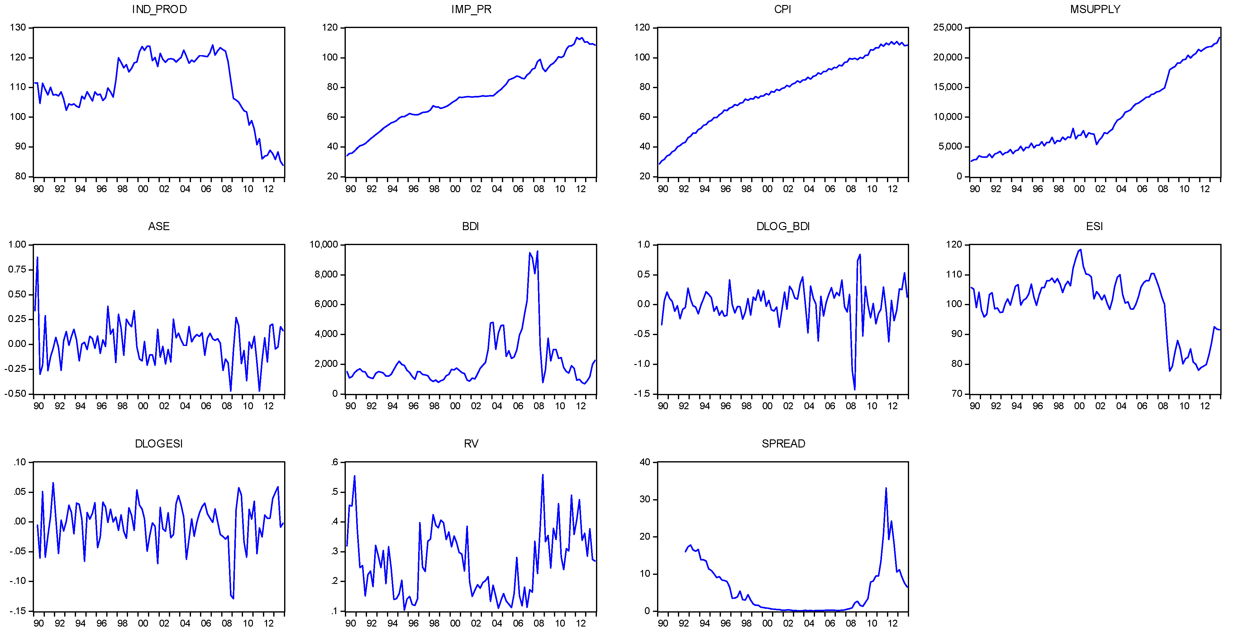
Quarterly data from 1990q1 to 2013q4 are available for a number of economic and financial variables; industrial production (IND_PROD), import prices (IMP_PR), consumer price index (CPI), money supply (MSUPPLY), Athens stock exchange index (ASE), Baltic Dry Cargo Index (BDI), log changes of BDI (DLOG_BDI), Economic Sentiment Indicator (ESI), log changes of ESI (DLOGESI), Realized volatility of ASE index (RV), and 10-year government bond spread (SPREAD). Figure 1 plots the variables, whereas Table 1 provides the descriptive statistics.

Figure 1. The explanatory variables: industrial production, import prices, CPI, money supply, Athens stock exchange (ASE) index, Baltic Dry Cargo Index (BDI), log changes of BDI, Economic Sentiment Indicator, log changes of ESI, Realized volatility of ASE index, and 10-year government bond spread. The sample period runs from 1990q1 to 2013q4.

Figure 1. The explanatory variables: industrial production, import prices, CPI, money supply, Athens stock exchange (ASE) index, Baltic Dry Cargo Index (BDI), log changes of BDI, Economic Sentiment Indicator, log changes of ESI, Realized volatility of ASE index, and 10-year government bond spread. The sample period runs from 1990q1 to 2013q4.

Table 1. Descriptive statistics of the explanatory variables.

	IND_PROD	IMP_PR	CPI	MSUPPLY	ASE	BDI
Mean	110.5	79.0	82.6	10,896.1	0.0	2325.3
Median	113.8	74.2	83.1	7858.5	0.0	1615.5
Maximum	124.3	113.6	110.9	23,366.0	0.4	9589.0
Minimum	83.8	46.7	43.2	3682.0	−0.5	699.0
Std. Dev.	11.5	18.3	18.7	6183.9	0.2	1906.0
Skewness	−0.8	0.3	−0.2	0.6	−0.4	2.3
Kurtosis	2.6	2.0	2.1	2.0	3.4	8.3
Jarque-Bera	9.9	4.7	3.8	10.0	2.8	178.7
Probability	0.007	0.097	0.146	0.007	0.243	0.000
	DLOG_BDI	ESI	DLOGESI	RV	SPREAD
Mean	0.0	99.9	0.0	0.3	5.8
Median	0.0	102.5	0.0	0.2	2.6
Maximum	0.8	118.5	0.1	0.6	33.1
Minimum	−1.4	77.8	−0.1	0.1	0.1
Std. Dev.	0.3	10.4	0.0	0.1	6.9
Skewness	−1.3	−0.8	−1.2	0.4	1.4
Kurtosis	8.2	2.6	5.5	2.3	4.9
Jarque-Bera	120.1	9.2	43.5	3.7	41.0
Probability	0.000	0.010	0.000	0.153	0.000

Table 1. Descriptive statistics of the explanatory variables.

	IND_PROD	IMP_PR	CPI	MSUPPLY	ASE	BDI
Mean	110.5	79.0	82.6	10,896.1	0.0	2325.3
Median	113.8	74.2	83.1	7858.5	0.0	1615.5
Maximum	124.3	113.6	110.9	23,366.0	0.4	9589.0
Minimum	83.8	46.7	43.2	3682.0	−0.5	699.0
Std. Dev.	11.5	18.3	18.7	6183.9	0.2	1906.0
Skewness	−0.8	0.3	−0.2	0.6	−0.4	2.3
Kurtosis	2.6	2.0	2.1	2.0	3.4	8.3
Jarque-Bera	9.9	4.7	3.8	10.0	2.8	178.7
Probability	0.007	0.097	0.146	0.007	0.243	0.000
	DLOG_BDI	ESI	DLOGESI	RV	SPREAD
Mean	0.0	99.9	0.0	0.3	5.8
Median	0.0	102.5	0.0	0.2	2.6
Maximum	0.8	118.5	0.1	0.6	33.1
Minimum	−1.4	77.8	−0.1	0.1	0.1
Std. Dev.	0.3	10.4	0.0	0.1	6.9
Skewness	−1.3	−0.8	−1.2	0.4	1.4
Kurtosis	8.2	2.6	5.5	2.3	4.9
Jarque-Bera	120.1	9.2	43.5	3.7	41.0
Probability	0.000	0.010	0.000	0.153	0.000

The spread is defined as the difference between the 10-year Greek and German bond yields. The annualized stock market realized volatility is computed as $S_{\text{t}}=\sqrt{4{\sum }_{d=1}^{n_t}{\left(r_{t,d}-{\overline{r}}_t\right)}^2}$, where $n_t$ is the number of days in quarter $t$, $r_{t,d}$ is the daily return of ASE (Athens General Stock Exchange Index) index in day $d$ of quarter $t$ and ${\overline{r}}_t=n_t^{-1}{\sum }_{d=1}^{n_t}{r}_{t,d}$. As noted in Degiannakis et al. [1], the current-looking volatility is accurately expressed by the realized volatility.

The Baltic Dry Cargo Index, issued daily by the London-based Baltic Exchange, provides an assessment of the price of moving the major raw materials by sea. The index measures the demand for shipping capacity versus the supply of dry bulk carriers. As the supply is generally inelastic, the BDI index is highly related with changes in demand. As Kilian and Hicks [2] note, the BDI belongs to the indices used by market practitioners for estimating the economic activity.

3. Two-State Regime Switching Model

A two-state regime-switching model for the log-differences of de-seasonalized GDP is estimated on a quarterly frequency (period 1990q1–2013q4) in the form 1:

$$\begin{array}{c}{y}_t={\text{μ}}_1+{\text{ε}}_{t,1},{\text{ ε}}_{t,1}~\text{N}\left(0,{\text{σ}}_{\epsilon }^2\right)\\ y_t={\text{μ}}_2+{\text{ε}}_{t,2},{\text{ ε}}_{t,2}~\text{N}\left(0,{\text{σ}}_{\text{ε}}^2\right),\end{array}$$

(1)

where $y_t$ is the q-o-q changes of log-GDP, ${\text{μ}}_j$ is the conditional mean for state j = 1,2, and ${\text{σ}}_{\text{ε}}^2$ denotes the variance of the normally distributed residuals 2. The log-GDP is assumed as a first order Markov process, described by a binary variable ${\text{S}}_t=1,2$ and the constant probabilities $p,q$ of remaining in Regime 1 or 2, respectively. The quality of regime classification measure, $RCM=400\frac{1}{T}{\sum }_{t=1}^T{p}_t\left(1-p_t\right)$ is evaluated according to Ang and Bekaert [9], where $p_t=P\left(S_t|I_T\right)$ for $I_T$ denoting the full sample information set. For the q-o-q GDP growth the $RCM$ measure equals to 18.2 providing strong indications that the regime switching model classifies correctly the periods of growth and recession; $RCM\ni \left[0,100\right]$ the lower the value indicates better regime classification.

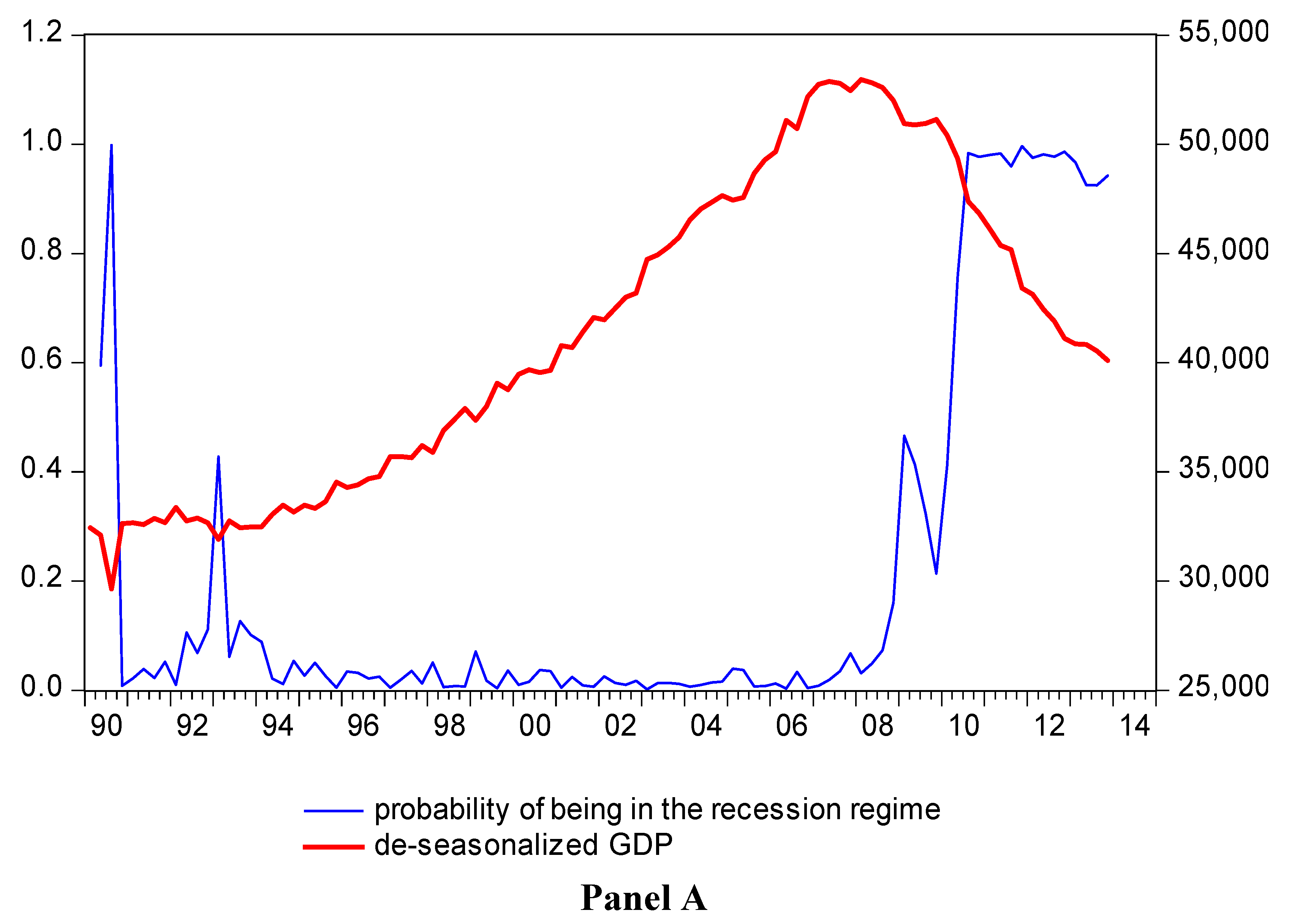
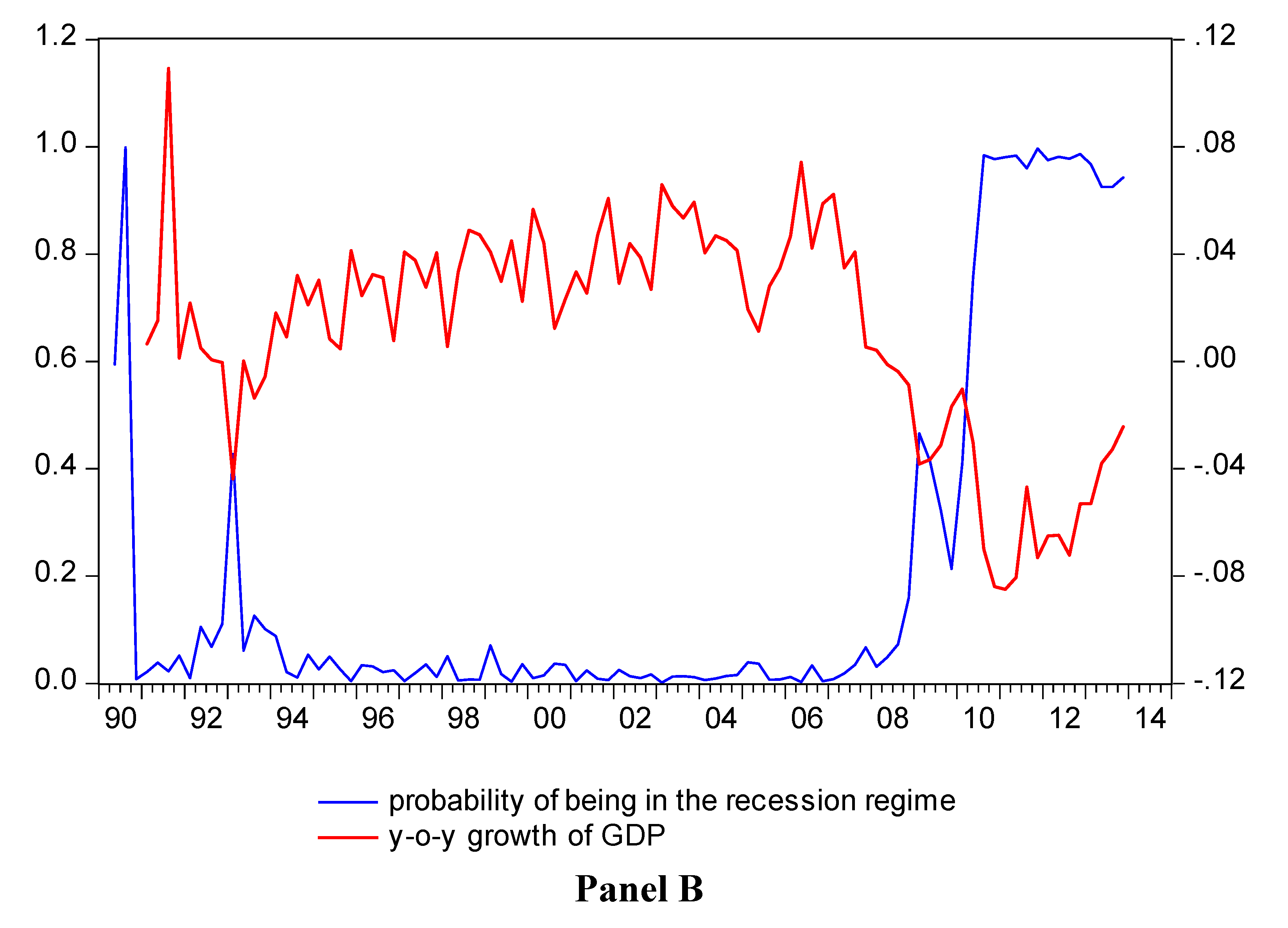
Figure 2 plots the probability 3 of State 2 (being in recession environment) along with the de-seasonalized GDP and the year-over-year (y-o-y) changes of GDP, whereas Table 2 provides the estimated coefficients of the model. The probability of being in recession is high for 1990q3 and for the period from 2010q2 up to the end of the sample. The probability of being in recession has been already increased from 2009q1. The regimes are quite persistent as the probability to stay in the growth or recession environment equals to 97.75% or 97.20%, respectively.

Figure 2. Panel A: Filtered probabilities of State 2 (being in the recession regime) in the left axis and the de-seasonalized GDP in the right axis. The sample period runs from 1990q1 to 2013q4. Panel B: Filtered probabilities of being in the recession regime (left axis) and the y-o-y growth of GDP (right axis).

Figure 2. Panel A: Filtered probabilities of State 2 (being in the recession regime) in the left axis and the de-seasonalized GDP in the right axis. The sample period runs from 1990q1 to 2013q4. Panel B: Filtered probabilities of being in the recession regime (left axis) and the y-o-y growth of GDP (right axis).

Table 2. The estimated coefficients of the regime switching model.

µ1	µ1	log(σ2)	$p$	q	RCM
0.00788 *	−0.015 *	−4.097154 *	97.75%	97.20%	18.2
(0.00216)	(0.00409)	(0.07706)

* denotes statistical significance at the 1%. Standard errors are reported in parentheses. The model is $y_t={\text{μ}}_j+{\text{ε}}_{t,j},{\text{ ε}}_{t,j}~\text{N}\left(0,{\text{σ}}_{\epsilon }^2\right)$, where $y_t$ is the q-o-q changes of log-GDP, ${\text{μ}}_j$ is the conditional mean for state j = 1,2, and ${\text{σ}}_{\text{ε}}^2$ denotes the variance of residuals. The sample period runs from 1990q1 to 2013q4.

Table 2. The estimated coefficients of the regime switching model.

µ1	µ1	log(σ2)	$p$	q	RCM
0.00788 *	−0.015 *	−4.097154 *	97.75%	97.20%	18.2
(0.00216)	(0.00409)	(0.07706)

* denotes statistical significance at the 1%. Standard errors are reported in parentheses. The model is $y_t={\text{μ}}_j+{\text{ε}}_{t,j},{\text{ ε}}_{t,j}~\text{N}\left(0,{\text{σ}}_{\epsilon }^2\right)$, where $y_t$ is the q-o-q changes of log-GDP, ${\text{μ}}_j$ is the conditional mean for state j = 1,2, and ${\text{σ}}_{\text{ε}}^2$ denotes the variance of residuals. The sample period runs from 1990q1 to 2013q4.

4. Probit Regression Model

To explore the ability of the explanatory variables under investigation to estimate the state of the GDP growth, we estimate the following probit regression 4:

$$P\left({\text{d}}_{\text{t}}=1\right)=\text{Φ}\left({\mathit{\beta }}_i{\mathit{X}}_t\right),$$

(2)

where d_t = 1 when the state probability is greater than 50%, and ${\text{d}}_{\text{t}}=0$ otherwise, and Φ is the cumulative distribution function of the standard normal distribution. The explanatory variables in vector ${\mathit{X}}_t$ include the macroeconomic and financial variables described in Section 2; i.e., industrial production, import prices, CPI, money supply, Athens stock exchange index, Baltic Dry Cargo Index and its log changes, Economic Sentiment Indicator and its log changes, Realized volatility of ASE index, and the 10-year government bond spread. The selection of the variables ${\mathit{X}}_t$ incorporated in the probit model is stepwise and is based on the minimization of the error in estimating the probability to be in Regime 1:

$$min\left(T^{-1}{{\displaystyle \sum }}_{t=1}^T\left|\text{Φ}\left({\widehat{\mathit{\beta }}}_i{\mathit{X}}_t\right)-p_t\right|\right)$$

(3)

Equation (3) is the mean absolute distance (MAD) between the probability of not being in recession and the probability estimated by the probit model. The specification that minimizes Equation (3) is:

$$P\left({\text{ d}}_{\text{t}}=1\right)=\text{Φ}\left(\begin{array}{c}-28.9+\\ \left(0.009\right)\end{array}\begin{array}{c}0.325 IND Pro{d}_t\\ \left(0.007\right)\end{array}\begin{array}{c}-12.57 R{V}_t\\ \left(0.029\right)\end{array}\right)$$

(4)

Two control variables provide significant explanatory power in predicting the contemporaneous state of Greek economy (as expressed by GDP); the industrial production and the realized volatility of ASE index.

The step-by-step inclusion/exclusion of the explanatory variables is conducted according to evaluation criterion in Equation (3). In Table 3 the evaluation criterion is presented as well as the p-values of the added explanatory variables. In the first step, one explanatory variable is incorporated in the probit model. All the variables are significant (except the ASE index and the log changes of BDI and ESI) with the expected signs. The industrial production provides the lowest mean absolute error (6.75%) in estimating the probability to be in Regime 1.

Table 3. Regression: $P\left({\text{ d}}_{\text{t}}=1\right)=\text{Φ}\left(\mathit{\beta }{\mathit{X}}_t\right)$, where ${\mathit{X}}_t$ denotes the vector of explanatory variables $\text{IND}\_{\text{PROD}}_t$, $\text{IMP}\_{\text{PR}}_t$, ${\text{CPI}}_t$, ${\text{MSUPPLY}}_t$, ${\text{ASE}}_t$, ${\text{BDI}}_t$, $\left(1-\text{L}\right){\text{logBDI}}_t, ES{I}_t$, $\left(1-\text{L}\right)\text{log}ES{I}_t$, $R{V}_t$, and ${\text{SPREAD}}_t.$ At each step one explanatory variable is incorporated in the model. The first column of each step provides the value of $\left(T^{-1}{\sum }_{t=1}^T\left|\text{Φ}\left({\widehat{\mathit{\beta }}}_i{\mathit{X}}_t\right)-p_t\right|\right)$. The values reported in parentheses denote the p-values. The sample period runs from 1990q1 to 2013q4.

Explanatory Variables	Step (1)		Step (2)		Step (3)
$\text{IND}\_{\text{PROD}}_t$	6.75%	(0.0003) ***
$\text{IMP}\_{\text{PR}}_t$	16.49%	(0.0000) ***	6.94%	(0.7179)	6.35%	(0.3645)
${\text{CPI}}_t$	19.73%	(0.0001) ***	7.03%	(0.6418)	6.36%	(0.3539)
${\text{MSUPPLY}}_t$	12.22%	(0.0000) ***	6.19%	(0.6153)	6.32%	(0.5589)
${\text{ASE}}_t$	26.34%	(0.8936)	6.49%	(0.1267)	6.44%	(0.1952)
${\text{BDI}}_t$	26.03%	(0.0716) *	7.41%	(0.3929)	6.58%	(0.2034)
$\left(1-\text{L}\right){\text{logBDI}}_t$	26.44%	(0.5867)	6.47%	(0.0996) *	6.48%	(0.3514)
$ES{I}_t$	10.92%	(0.0000) ***	5.78%	(0.5060)	6.50%	(0.5898)
$\left(1-\text{L}\right)\text{log}ES{I}_t$	26.35%	(0.8016)	6.08%	(0.2469)	6.39%	(0.8678)
$R{V}_t$	21.47%	(0.0003) ***	6.43%	(0.0291) **
${\text{SPREAD}}_t$	19.14%	(0.0000) ***	(na)	(na)	(na)	(na)

Note: ***, ** and * denote statistical significance at the 1%, 5% and the 10% level, respectively. White’s [12] robust standard errors have been computed.

Table 3. Regression: $P\left({\text{ d}}_{\text{t}}=1\right)=\text{Φ}\left(\mathit{\beta }{\mathit{X}}_t\right)$, where ${\mathit{X}}_t$ denotes the vector of explanatory variables $\text{IND}\_{\text{PROD}}_t$, $\text{IMP}\_{\text{PR}}_t$, ${\text{CPI}}_t$, ${\text{MSUPPLY}}_t$, ${\text{ASE}}_t$, ${\text{BDI}}_t$, $\left(1-\text{L}\right){\text{logBDI}}_t, ES{I}_t$, $\left(1-\text{L}\right)\text{log}ES{I}_t$, $R{V}_t$, and ${\text{SPREAD}}_t.$ At each step one explanatory variable is incorporated in the model. The first column of each step provides the value of $\left(T^{-1}{\sum }_{t=1}^T\left|\text{Φ}\left({\widehat{\mathit{\beta }}}_i{\mathit{X}}_t\right)-p_t\right|\right)$. The values reported in parentheses denote the p-values. The sample period runs from 1990q1 to 2013q4.

Explanatory Variables	Step (1)		Step (2)		Step (3)
$\text{IND}\_{\text{PROD}}_t$	6.75%	(0.0003) ***
$\text{IMP}\_{\text{PR}}_t$	16.49%	(0.0000) ***	6.94%	(0.7179)	6.35%	(0.3645)
${\text{CPI}}_t$	19.73%	(0.0001) ***	7.03%	(0.6418)	6.36%	(0.3539)
${\text{MSUPPLY}}_t$	12.22%	(0.0000) ***	6.19%	(0.6153)	6.32%	(0.5589)
${\text{ASE}}_t$	26.34%	(0.8936)	6.49%	(0.1267)	6.44%	(0.1952)
${\text{BDI}}_t$	26.03%	(0.0716) *	7.41%	(0.3929)	6.58%	(0.2034)
$\left(1-\text{L}\right){\text{logBDI}}_t$	26.44%	(0.5867)	6.47%	(0.0996) *	6.48%	(0.3514)
$ES{I}_t$	10.92%	(0.0000) ***	5.78%	(0.5060)	6.50%	(0.5898)
$\left(1-\text{L}\right)\text{log}ES{I}_t$	26.35%	(0.8016)	6.08%	(0.2469)	6.39%	(0.8678)
$R{V}_t$	21.47%	(0.0003) ***	6.43%	(0.0291) **
${\text{SPREAD}}_t$	19.14%	(0.0000) ***	(na)	(na)	(na)	(na)

Note: ***, ** and * denote statistical significance at the 1%, 5% and the 10% level, respectively. White’s [12] robust standard errors have been computed.

In the second step, the industrial production index and one more explanatory variable is incorporated in the model. All the additional variables are insignificant (except the log changes of BDI and the Realized Volatility of Athens stock market) but with the expected signs. The model with the industrial production index and the realized volatility as explanatory variables achieves the lowest value (6.43%) of the evaluation criterion in Equation (3). In the third step, all the additional variables are statistically insignificant. Therefore, we conclude with the model of the second step.

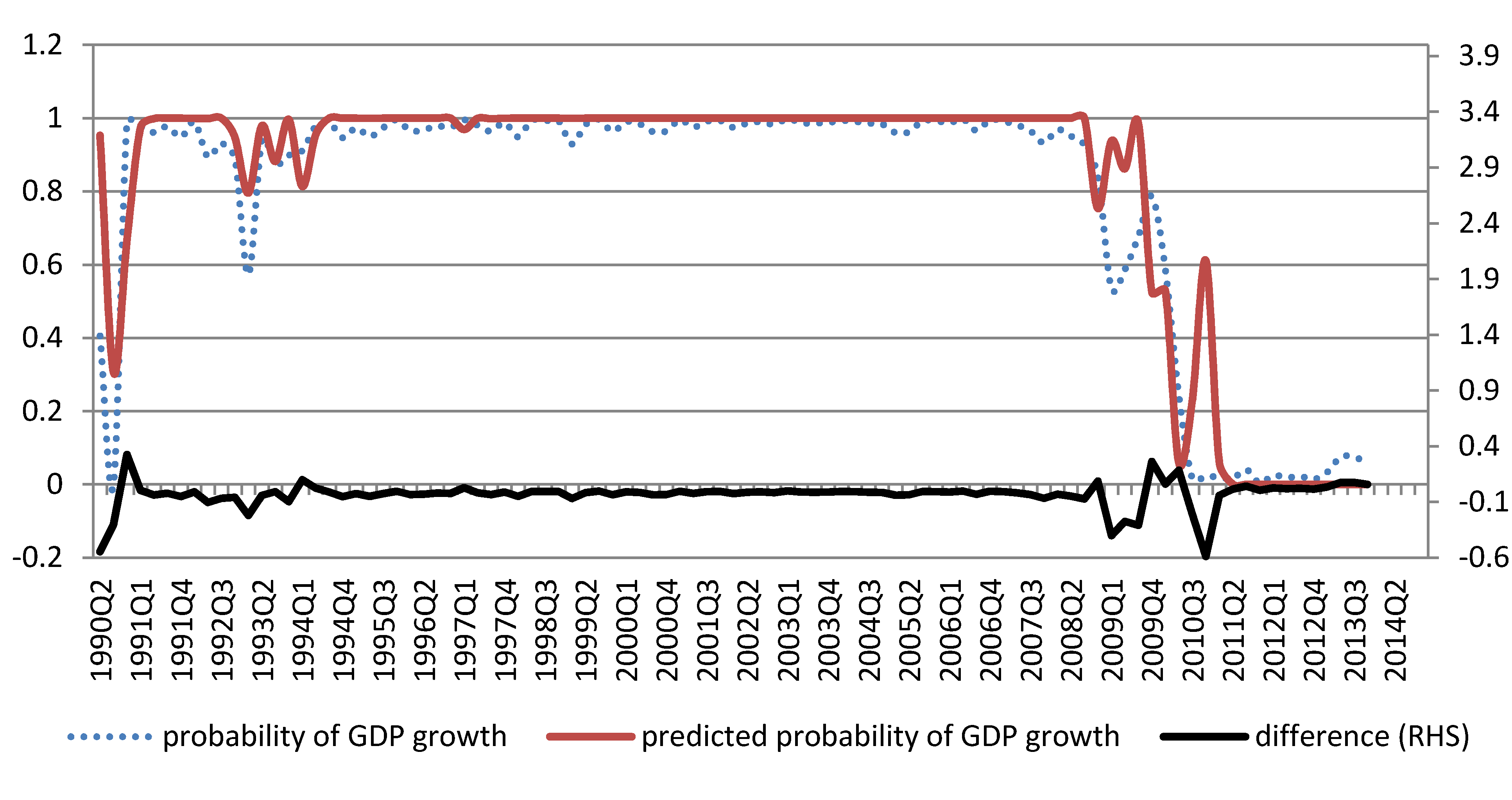
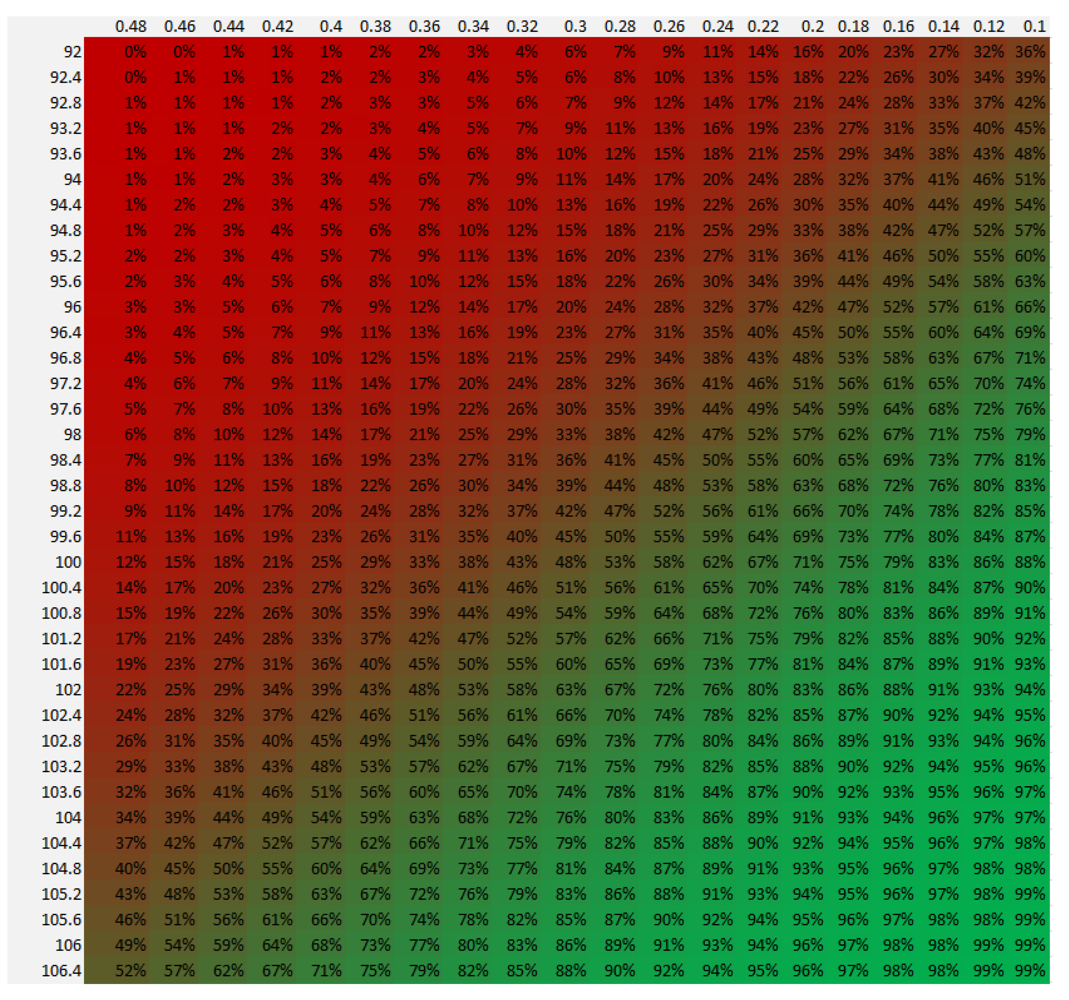
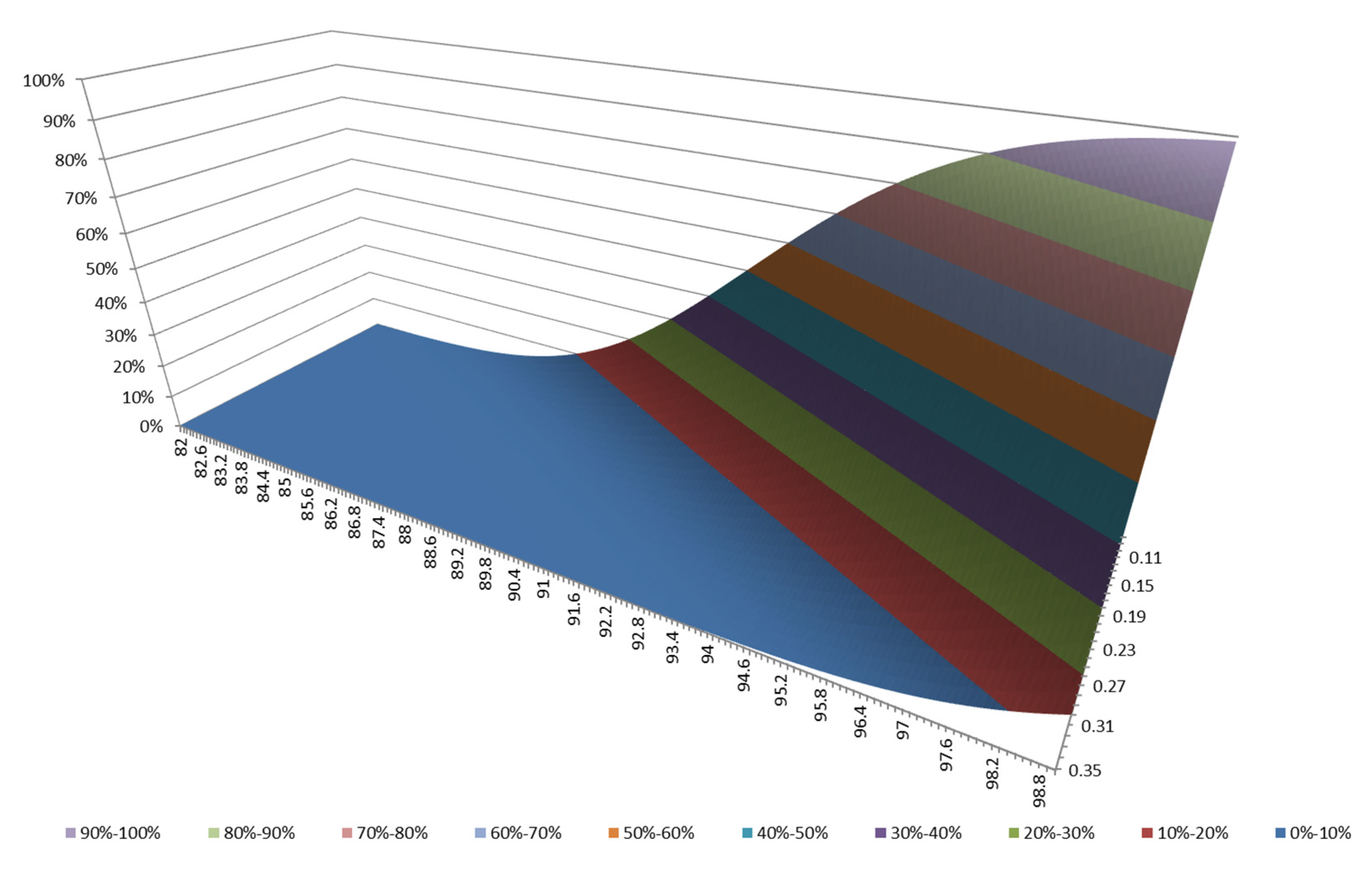
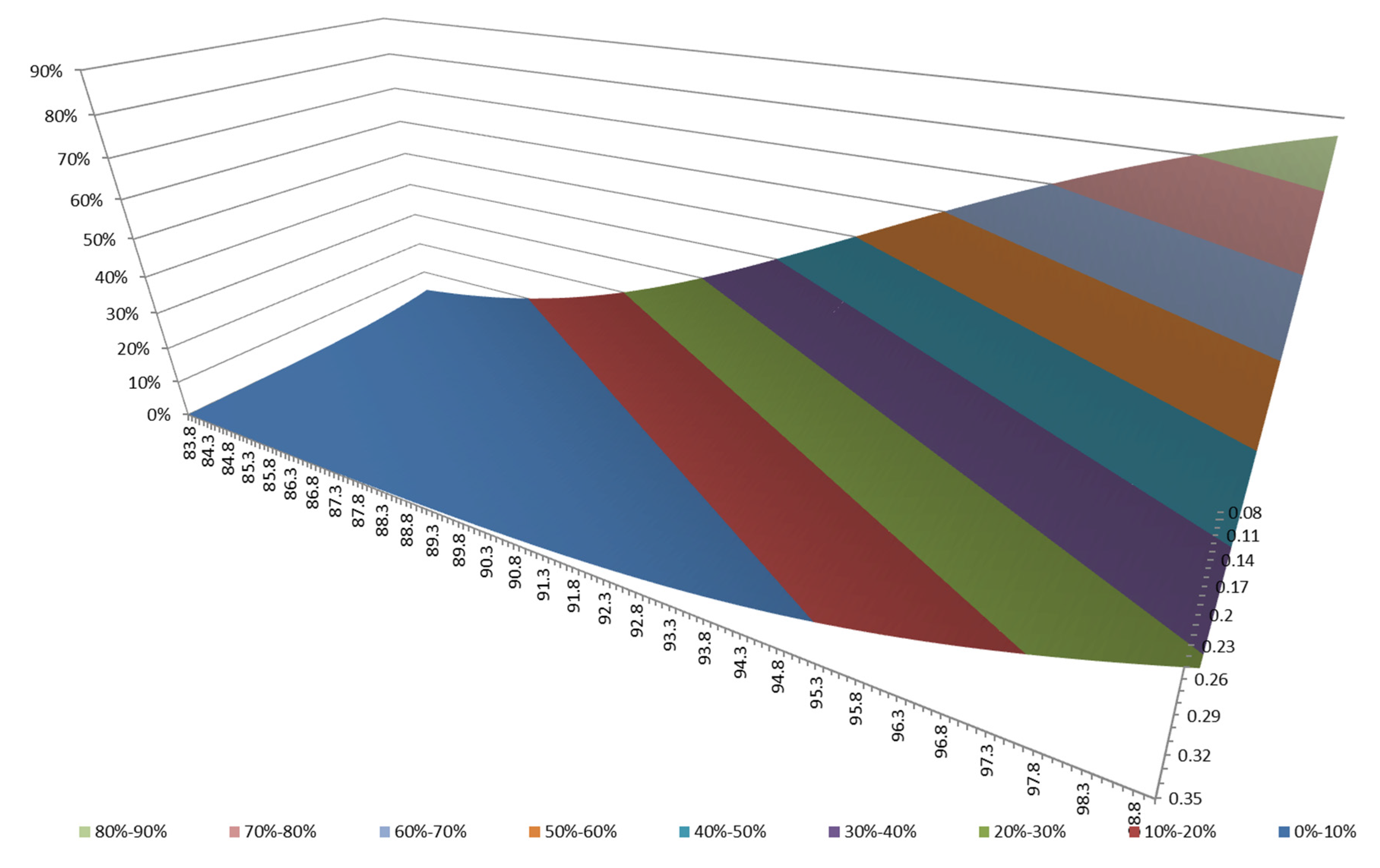
Figure 3 plots the probability of GDP being in boom state (${\text{ d}}_{\text{t}}=1$) along with its estimate based on Equation (4). Although the changes (from the boom state into a recession period) in the Greek GDP are not characterized for their smoothness, the model does capture the onset of recession in 2009. Naturally, the performance of the models is not the best at such points in time. Figure 4 plots the projected probability of GDP being in boom state (${\text{ d}}_{\text{t}}=1$) for various values of the industrial production and the ASE realized volatility.

Figure 3. Filtered probability of GDP being in boom state (d_t = 1) along with its estimate. The sample period runs from 1990q1 to 2013q4.

Figure 3. Filtered probability of GDP being in boom state (d_t = 1) along with its estimate. The sample period runs from 1990q1 to 2013q4.

Figure 4. For 2014q1, the projected probability of GDP being in boom state (d_t = 1) for various values of industrial production (82–99) and realized volatility of ASE stock index (11%–35%).

Figure 4. For 2014q1, the projected probability of GDP being in boom state (d_t = 1) for various values of industrial production (82–99) and realized volatility of ASE stock index (11%–35%).

5. Lagged Relationship

In this case, we focus on the lagged relationship between the state of GDP growth and explanatory variables, the probit model is $P\left({\text{ d}}_{\text{t}}=1\right)=\text{Φ}\left({\mathit{\beta }}_i{\mathit{X}}_{t-1}\right)$, and the selection of the variables incorporated in the model is conducted based on the minimisation of the $min\left({\left(T-1\right)}^{-1}\sum _{t=2}^T\left|\text{Φ}\left({\widehat{\mathit{\beta }}}_i{\mathit{X}}_{t-1}\right)-p_t\right|\right)$ evaluation function.

The most adequate specification is:

$$P\left({\text{ d}}_{\text{t}}=1\right)=\text{Φ}\left(\begin{array}{c}-17.43+\\ \left(0.002\right)\end{array}\begin{array}{c}0.192 IND Pro{d}_{t-1}\\ \left(0.0004\right)\end{array}\begin{array}{c}-6.195 R{V}_{t-1}\\ \left(0.027\right)\end{array}\right)$$

(5)

As in the case of the contemporaneous relationship, the industrial production and the realized volatility of ASE index provide the major explanatory power in predicting the contemporaneous state of the Greek economy (as expressed by GDP).

The step-by-step inclusion/exclusion of the explanatory variables is presented in Table 4. In the first step, where one explanatory variable is incorporated in the model, all the variables are significant (except the ASE index, the BDI index and its log changes, and the log changes of ESI) with the expected signs. The industrial production provides the lowest mean absolute error (9.31%) in estimating the probability to be in regime 1.

Table 4. Regression: $P\left({\text{ d}}_{\text{t}}=1\right)=\text{Φ}\left(\mathit{\beta }{\mathit{X}}_{t-1}\right)$, where ${\mathit{X}}_t$ denotes the vector of explanatory variables $\text{IND}\_{\text{PROD}}_t$, $\text{IMP}\_{\text{PR}}_t$, ${\text{CPI}}_t$, ${\text{MSUPPLY}}_t$, ${\text{ASE}}_t$, ${\text{BDI}}_t$, $\left(1-\text{L}\right){\text{logBDI}}_t, ES{I}_t$, $\left(1-\text{L}\right)\text{log}ES{I}_t$, $R{V}_t$, and ${\text{SPREAD}}_t.$ At each step one explanatory variable is incorporated in the model. The first column of each step provides the value of $\left(T^{-1}\sum _{t=1}^T\left|\text{Φ}\left({\widehat{\mathit{\beta }}}_i{\mathit{X}}_{t-1}\right)-p_t\right|\right)$. The values reported in parentheses denote the p-values. The sample period runs from 1990q1 to 2013q4.

Explanatory Variables	Step (1)		Step (2)		Step (3)
$\text{IND}\_{\text{PROD}}_{t-1}$	9.31%	(0.0001) ***
$\text{IMP}\_{\text{PR}}_{t-1}$	16.36%	(0.0000) ***	8.42%	(0.5197)	7.70%	(0.8471)
${\text{CPI}}_{t-1}$	19.54%	(0.0001) ***	8.75%	(0.6856)	7.90%	(0.9752)
${\text{MSUPPLY}}_{t-1}$	11.89%	(0.0000) ***	6.95%	(0.1241)	6.96%	(0.4613)
${\text{ASE}}_{t-1}$	25.96%	(0.6993)	8.93%	(0.0241) **	7.84%	(0.1381)
${\text{BDI}}_{t-1}$	25.69%	(0.1041)	8.92%	(0.7026)	7.83%	(0.8189)
$\left(1-\text{L}\right){\text{logBDI}}_{t-1}$	25.32%	(0.4772)	7.92%	(0.0610) *	7.21%	(0.2207)
$ES{I}_{t-1}$	10.43%	(0.0000) ***	7.55%	(0.2780)	7.62%	(0.8205)
$\left(1-\text{L}\right)\text{log}ES{I}_{t-1}$	25.56%	(0.6349)	8.24%	(0.3905)	7.80%	(0.9654)
$R{V}_{t-1}$	20.90%	(0.0004) ***	7.94%	(0.0274) **
${\text{SPREAD}}_{t-1}$	20.15%	(0.0000) ***	(na)	(na)	(na)	(na)

Note: ***, ** and * denote statistical significance at the 1%, 5% and the 10% level, respectively. White’s [12] robust standard errors have been computed.

Table 4. Regression: $P\left({\text{ d}}_{\text{t}}=1\right)=\text{Φ}\left(\mathit{\beta }{\mathit{X}}_{t-1}\right)$, where ${\mathit{X}}_t$ denotes the vector of explanatory variables $\text{IND}\_{\text{PROD}}_t$, $\text{IMP}\_{\text{PR}}_t$, ${\text{CPI}}_t$, ${\text{MSUPPLY}}_t$, ${\text{ASE}}_t$, ${\text{BDI}}_t$, $\left(1-\text{L}\right){\text{logBDI}}_t, ES{I}_t$, $\left(1-\text{L}\right)\text{log}ES{I}_t$, $R{V}_t$, and ${\text{SPREAD}}_t.$ At each step one explanatory variable is incorporated in the model. The first column of each step provides the value of $\left(T^{-1}\sum _{t=1}^T\left|\text{Φ}\left({\widehat{\mathit{\beta }}}_i{\mathit{X}}_{t-1}\right)-p_t\right|\right)$. The values reported in parentheses denote the p-values. The sample period runs from 1990q1 to 2013q4.

Explanatory Variables	Step (1)		Step (2)		Step (3)
$\text{IND}\_{\text{PROD}}_{t-1}$	9.31%	(0.0001) ***
$\text{IMP}\_{\text{PR}}_{t-1}$	16.36%	(0.0000) ***	8.42%	(0.5197)	7.70%	(0.8471)
${\text{CPI}}_{t-1}$	19.54%	(0.0001) ***	8.75%	(0.6856)	7.90%	(0.9752)
${\text{MSUPPLY}}_{t-1}$	11.89%	(0.0000) ***	6.95%	(0.1241)	6.96%	(0.4613)
${\text{ASE}}_{t-1}$	25.96%	(0.6993)	8.93%	(0.0241) **	7.84%	(0.1381)
${\text{BDI}}_{t-1}$	25.69%	(0.1041)	8.92%	(0.7026)	7.83%	(0.8189)
$\left(1-\text{L}\right){\text{logBDI}}_{t-1}$	25.32%	(0.4772)	7.92%	(0.0610) *	7.21%	(0.2207)
$ES{I}_{t-1}$	10.43%	(0.0000) ***	7.55%	(0.2780)	7.62%	(0.8205)
$\left(1-\text{L}\right)\text{log}ES{I}_{t-1}$	25.56%	(0.6349)	8.24%	(0.3905)	7.80%	(0.9654)
$R{V}_{t-1}$	20.90%	(0.0004) ***	7.94%	(0.0274) **
${\text{SPREAD}}_{t-1}$	20.15%	(0.0000) ***	(na)	(na)	(na)	(na)

Note: ***, ** and * denote statistical significance at the 1%, 5% and the 10% level, respectively. White’s [12] robust standard errors have been computed.

In the second step, the industrial production index and one more explanatory variable are incorporated in the model. All the additional variables are insignificant (except the ASE index and its realized volatility) but with the expected signs. The model with the industrial production index and the realized volatility as explanatory variables achieves the lowest value (7.94%) of the evaluation criterion. In the third step, all the additional variables are statistically insignificant. Therefore, we conclude with the model of the second step.

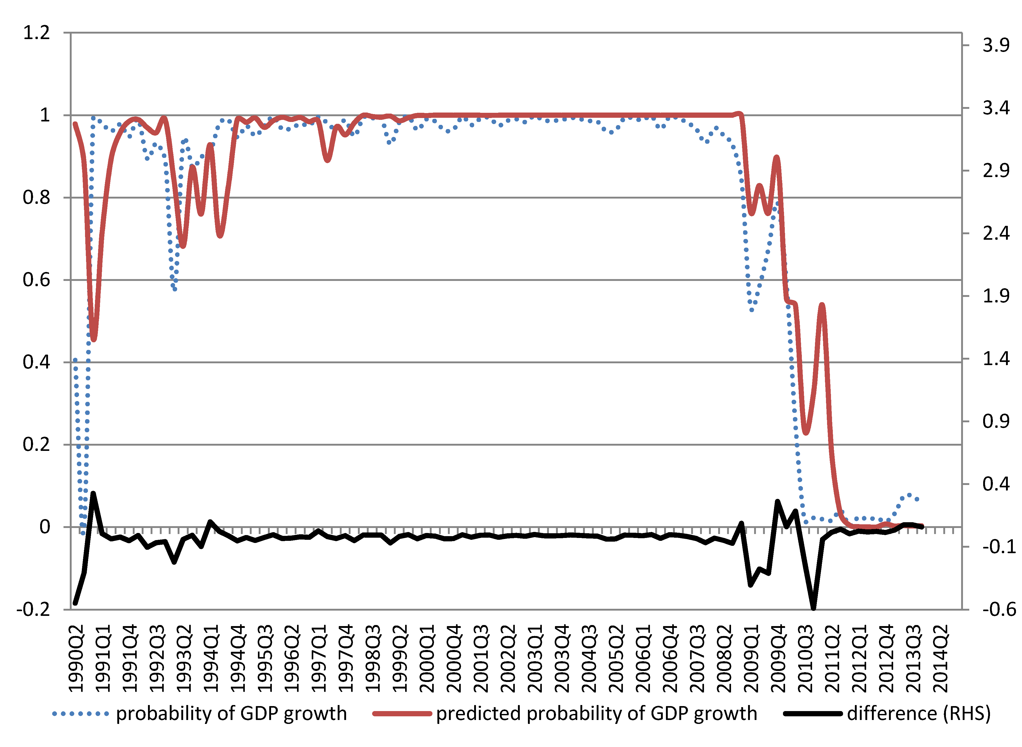
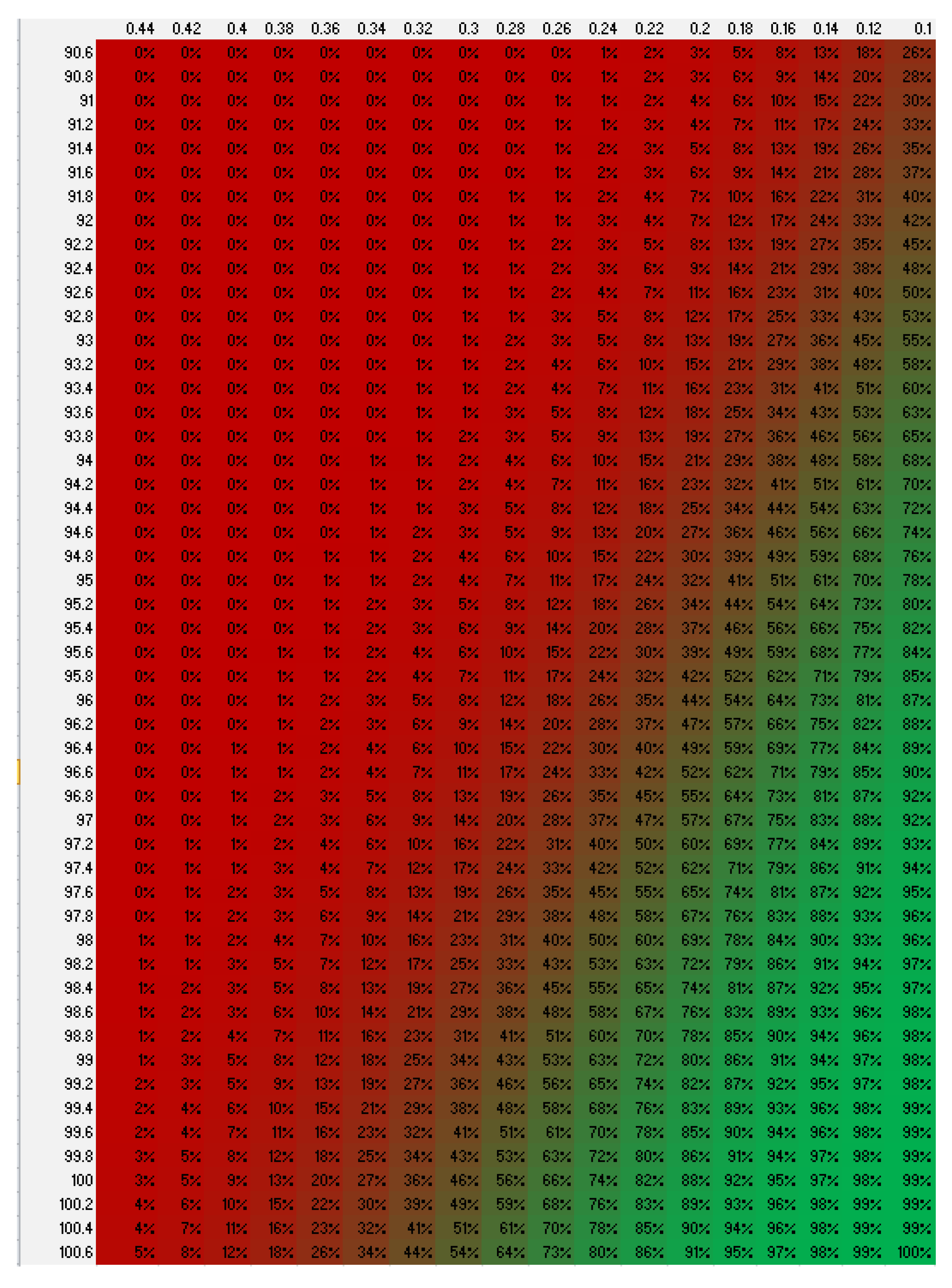
Figure 5 plots the probability of GDP being in boom state (${\text{ d}}_{\text{t}}=1$) along with its forecast based on Equation (5). Figure 6 plots the projected probability of GDP being in boom state (${\text{ d}}_{\text{t}}=1$) for various values of industrial production and the realized volatility of ASE index.

Figure 5. Probability of GDP being in boom state (${\text{ d}}_{\text{t}}=1$) along with its forecast. The sample period runs from 1990q1 to 2013q4.

Figure 5. Probability of GDP being in boom state (${\text{ d}}_{\text{t}}=1$) along with its forecast. The sample period runs from 1990q1 to 2013q4.

Figure 6. For 2014q1, the projected probability of GDP being in boom state (${\text{ d}}_{\text{t}}=1$) for various values of industrial production (82–99) and the ASE realized volatility (11%–35%).

Figure 6. For 2014q1, the projected probability of GDP being in boom state (${\text{ d}}_{\text{t}}=1$) for various values of industrial production (82–99) and the ASE realized volatility (11%–35%).

6. Conclusions

The present study provided strong empirical evidence that the probability of Greek GDP being in recession or boom can be estimated (both in terms of now-casting and short-term forecasting) by macroeconomic and financial variables. The sign of the q-o-q GDP growth is predictable via a probit model by the industrial production index and the Athens stock market realized volatility. The mean absolute distance between the probability of being in boom and the probability estimated by the probit model is 6.43% and 7.94% in the contemporaneous and the lagged relationships, respectively.

For future study we seek to investigate whether any additional set of macroeconomic and financial variables is able to enhance the forecasting accuracy. It would also be interesting to have an out-of-sample forecasting exercise by updating the estimation of models’ parameters at each quarter. Moreover, the examination of contemporaneous or lagged relationship between economic/financial variables and the state of the GDP growth must be conducted for other economies as well.