Is Loan Diversification Always Beneficial? Nonlinear Evidence from Vietnamese Commercial Banks

Abstract

This study investigates the nonlinear relationship between sectoral loan diversification and credit risk in Vietnamese commercial banks. Using a balanced panel of 14 banks over 2012–2025, comprising 196 bank-year observations, the study measures diversification through a Shannon Entropy Index based on a harmonized ten-sector classification and measures credit risk using the reported non-performing loan ratio. The relationship is examined using conventional panel estimators, two-step System GMM, and bias-corrected LSDV models, together with alternative diversification measures. The results provide suggestive evidence of a U-shaped association: diversification is associated with lower credit risk at relatively low levels but with higher credit risk beyond a conditional turning point. This pattern is supported by the System GMM and small-sample bias-corrected estimates, although it is not statistically robust to the HHI-based measure. The findings therefore indicate that the effects of diversification depend on both its extent and measurement and should not be interpreted as identifying a universal optimal threshold. Banks and supervisors should assess sectoral diversification alongside cross-sector risk correlations, underwriting expertise, and monitoring capacity.

1. Introduction

Commercial banks play a central role in promoting economic growth by mobilizing savings and allocating credit to productive sectors. However, their contribution to economic development largely depends on maintaining sound asset quality and effective credit risk management. Among various indicators of banking stability, non-performing loans (NPLs) have attracted considerable attention because they directly affect bank profitability, capital adequacy, liquidity, and lending capacity. A persistent increase in NPLs not only weakens the financial performance of individual banks but also undermines financial stability and constrains economic growth through the credit channel (Berger & DeYoung, 1997; Beck et al., 2015; IMF, 2021). Consequently, identifying effective strategies to reduce credit risk has become an important issue for both banking practitioners and policymakers.

The Vietnamese banking sector provides a relevant setting for examining this relationship. Over the study period, banks operated through major changes in economic conditions, including banking-sector restructuring, the COVID-19 shock, and subsequent stress in the real estate and corporate bond markets. At the same time, the Law on Credit Institutions No. 32/2024/QH15 has reinforced regulatory attention to credit concentration and internal risk governance (National Assembly of Vietnam, 2024). Although its large-exposure provisions apply primarily to individual customers and related customer groups rather than sectoral loan allocation, the Law reflects a broader policy concern with the risks arising from concentrated credit portfolios. Against this background, understanding whether sectoral diversification consistently reduces credit risk—or produces different effects at different levels—has become increasingly relevant to both bank managers and supervisors.

The relationship between loan diversification and bank risk remains theoretically and empirically inconclusive (Acharya et al., 2006; Hayden et al., 2007; Rossi et al., 2009). According to Modern Portfolio Theory (Markowitz, 1952), diversification reduces idiosyncratic risk by allocating assets across imperfectly correlated investments, implying that broader loan portfolios should enhance banking stability. Similar arguments have been developed in banking studies, suggesting that diversified lending reduces concentration risk and improves banks’ resilience against sector-specific shocks (Diamond, 1984; Tabak et al., 2011; Shim, 2019). In contrast, the focus hypothesis argues that excessive diversification may weaken banks’ informational advantages and increase monitoring costs. Expanding lending into unfamiliar industries can reduce screening quality, intensify information asymmetry, and increase adverse selection problems, ultimately deteriorating loan quality (Winton, 1999; Acharya et al., 2006; Hayden et al., 2007; Elsas et al., 2010). Consequently, diversification may improve bank performance only up to a certain point, beyond which its benefits gradually diminish (Winton, 1999; Acharya et al., 2006; Huynh & Dang, 2022).

Empirical findings are mixed partly because studies examine different outcomes—including NPLs, loan-loss provisions, profitability, insolvency risk, and risk-adjusted performance—and use different diversification measures. These outcomes are not interchangeable. The present study focuses narrowly on reported NPLs and evaluates whether their conditional association with sectoral dispersion is nonlinear. It does not claim that all prior research assumes linearity; rather, it tests whether a quadratic pattern is informative in this specific emerging-market setting.

This study contributes in three qualified respects. First, it constructs a harmonized sectoral loan-allocation measure for a balanced panel of Vietnamese banks. Second, it tests a nonlinear association with reported NPLs and reports uncertainty around a sample-specific turning point. Third, it compares the results across conventional panel estimators, System GMM, bias-corrected LSDV, normalized entropy, and HHI-based diversification. The contribution is therefore comparative and conditional, not a claim of being the first study to establish a universal diversification threshold.

The remainder of the paper is structured as follows. Section 2 reviews the literature and develops the hypotheses. Section 3 describes the data, variables, and empirical strategy. Section 4 presents the results and robustness analyses. Section 5 concludes and discusses implications and limitations.

2. Literature Review and Hypothesis Development

2.1. Loan Portfolio Diversification and Credit Risk

Non-performing loans (NPLs) directly capture recognized deterioration in loan quality, but they differ from broader measures such as loan-loss provisions, reserves, profitability, and insolvency risk (Berger & DeYoung, 1997; Louzis et al., 2012). Reported NPLs reflect both borrower performance and accounting or regulatory classification. Sectoral diversification may affect NPLs through the dispersion of sector-specific shocks, changes in screening quality, and the organizational demands imposed on monitoring systems.

The first mechanism is risk dispersion. When sectoral cash flows are imperfectly correlated, spreading loans across sectors can reduce exposure to a single-sector shock (Markowitz, 1952; Diamond, 1984; BCBS, 2000; Tabak et al., 2011). Evidence on risk-adjusted performance, stability, or provisions is relevant to this mechanism but should not be interpreted automatically as direct evidence about NPL ratios (Elsas et al., 2010; Rossi et al., 2009; Shim, 2019; Behr et al., 2007).

The second mechanism concerns information advantages and relationship lending. Specialization allows banks to accumulate sector-specific knowledge, thereby improving borrower screening and the early detection of financial distress (Winton, 1999; Berger & Udell, 2002; Kamp et al., 2005). The third mechanism relates to organizational complexity. Expanding lending activities into unfamiliar sectors may increase information-acquisition and monitoring costs and place greater demands on managerial capacity (Cerasi & Daltung, 2000; Acharya et al., 2006; Hayden et al., 2007). Consequently, as a loan portfolio becomes more broadly diversified, the loss of sector-specific expertise and the increasing complexity of credit monitoring may gradually offset the initial benefits of risk dispersion.

These mechanisms can generate nonlinearity (Winton, 1999; Acharya et al., 2006; Huynh & Dang, 2022). At relatively low levels of diversification, the marginal benefit from reducing sector concentration may dominate. At higher levels, additional risk dispersion may be offset by weaker sector expertise and greater organizational complexity. Nevertheless, sectoral dispersion is not synonymous with true economic-risk diversification: exposures classified in different industries may remain correlated through common collateral, borrower groups, supply chains, geographic concentration, or macroeconomic sensitivity.

The empirical question is therefore whether the marginal association changes over the observed diversification range. A quadratic model offers a parsimonious way to examine this possibility, but it imposes a restrictive symmetric functional form. The estimated curve and turning point must consequently be interpreted as model-dependent and evaluated through formal boundary slopes and alternative measures.

2.2. Hypothesis Development

The preceding literature suggests that the relationship between loan portfolio diversification and credit risk is theoretically ambiguous. The diversification hypothesis argues that spreading credit exposures across different industries, borrower groups, and geographic regions reduces concentration risk and limits the impact of sector-specific shocks on banks’ loan portfolios (Markowitz, 1952; BCBS, 2000). By lowering the likelihood of simultaneous borrower defaults, diversification is expected to improve loan quality and reduce non-performing loans.

Conversely, the focus hypothesis suggests that excessive diversification may undermine banks’ informational advantages and weaken credit risk management. As banks expand lending into unfamiliar sectors, they incur higher information acquisition costs, face greater monitoring complexity, and may experience a deterioration in screening quality (Winton, 1999; Stiglitz & Weiss, 1981; Acharya et al., 2006; Hayden et al., 2007). These challenges can weaken lending standards and increase the probability of borrower default, ultimately leading to higher non-performing loans (Acharya et al., 2006).

Together, these arguments imply two directional hypotheses stated in associational rather than causal terms.

H1. 

At relatively low levels of sectoral loan diversification, greater diversification is associated with a lower non-performing loan ratio.

At higher levels of sectoral dispersion, declining informational advantages and increasing monitoring complexity may outweigh the marginal benefits of risk dispersion.

The second hypothesis therefore concerns the full shape of the relationship within the observed range.

H2. 

The relationship between sectoral loan diversification and the non-performing loan ratio is U-shaped, such that its marginal association becomes positive beyond a conditional turning point.

3. Data and Methodology

3.1. Sample and Data Sources

The study employs a balanced panel of 14 Vietnamese commercial banks from 2012 to 2025, comprising 196 bank-year observations. The data were collected from audited consolidated annual financial statements and accompanying notes, including full-year reports for 2025. Banks were selected based on the consistent availability of sectoral lending data; consequently, the sample may not be fully representative of the entire Vietnamese banking system.

The period spans banking-sector restructuring, relatively stable pre-pandemic growth, the COVID-19 shock, corporate-bond and real-estate stress, and the introduction of the 2024 Law on Credit Institutions. The law is treated solely as institutional context; the models are not designed to estimate its causal effect. Appendix A identifies the banks, ownership grouping, fiscal-year coverage, and reporting basis.

Loan portfolio diversification is measured using the Shannon Entropy Index (SE), calculated from a fixed, harmonized classification of ten sector groups for every bank-year. Sector shares are measured relative to gross customer loans and are checked to sum to one, subject to rounding. A disclosed zero exposure is retained as zero; an undisclosed exposure is not automatically treated as zero. The index is defined as follows:

$${SE}_{it}=-{\displaystyle \sum _{k=1}^n}{p}_{k,it}\mathrm{l}\mathrm{n}(p_{k,it})$$

where p_k,it is the share of gross customer loans allocated to harmonized sector k by bank i in year t, and K = 10. Higher SE indicates greater sectoral dispersion. Because raw entropy is bounded by ln(K), normalized entropy is also calculated as SE_norm,it = SE_it/ln(10). As an alternative measure, HHI-based diversification is defined as DIV_HHI_it = 1 − ${\displaystyle {\sum }_{k=1}^K}{p}_{k,it}^2$. Sectoral dispersion does not necessarily capture common collateral, borrower-group, geographic, or supply-chain risk.

Bank-specific data were collected from audited consolidated annual financial statements and accompanying notes published by the banks. Macroeconomic variables were obtained from the General Statistics Office of Vietnam and the World Development Indicators. NPL is measured as loans classified in Groups 3–5 divided by gross customer loans, based on consolidated financial statements. Although this measure is consistently available across the sampled banks, it may not fully capture underlying credit risk. In particular, transfers of impaired loans to the Vietnam Asset Management Company and regulatory loan-restructuring arrangements may affect the timing with which credit deterioration is recognized in reported NPLs. Because comparable bank-level information on these exposures is unavailable for the entire sample period, a consistently adjusted NPL measure cannot be constructed. This limitation is considered when interpreting the empirical results.

Table 1. Variable definitions.

Variable	Symbol	Measurement	Expected Sign	References
Non-performing loan ratio	NPL	Loans classified in Groups 3–5/gross customer loans; consolidated basis; off-balance-sheet exposures excluded	Dependent	Berger and DeYoung (1997); Louzis et al. (2012)
Loan portfolio diversification	SE	Shannon Entropy Index	− at relatively low levels	Acharya et al. (2006); Shim (2019); Huynh and Dang (2022)
Diversification squared	SE2	Square of Shannon Entropy Index	+ under H2
Bank size	SIZE	ln(Total assets)	±	Louzis et al. (2012)
Capital ratio	CAP	Equity/Total assets	–	Berger and DeYoung (1997)
Credit growth	CRG	Annual growth rate of total loans	+	Foos et al. (2010)
Profitability	ROE	Net income/Equity	–	Louzis et al. (2012)
GDP growth	GDP	Annual GDP growth (%)	–	Louzis et al. (2012)
Inflation	INF	Annual inflation rate (%)	+	Nkusu (2011); Klein (2013)

Source: Authors’ synthesis.

defines the variables. SE and its squared term capture the hypothesized nonlinear association. Bank-level controls comprise size, capital, credit growth, and ROE; GDP growth and inflation capture common annual macroeconomic conditions. Because the macro variables vary only by year, they are not included jointly with a full set of year indicators in the reported GMM model.

3.2. Empirical Model

To examine the impact of loan portfolio diversification on bank credit risk, the following baseline empirical model is specified:

$$\begin{array}{l}{\mathrm{NPL}}_{it}={\beta }_0+{\beta }_1{\mathrm{SE}}_{it}+{\beta }_2{\mathrm{SE}}_{it}^2+{\beta }_3{\mathrm{CAP}}_{it}+{\beta }_4{\mathrm{SIZE}}_{it}+{\beta }_5{\mathrm{CRG}}_{it}+{\beta }_6{\mathrm{ROE}}_{it}+{\beta }_7{\mathrm{GDP}}_t\\ +{\beta }_8{\mathrm{INF}}_t+{\mu }_i+{\epsilon }_{it}\end{array}$$

where NPL is the reported non-performing loan ratio; SE and SE² represent sectoral diversification and its quadratic term; SIZE, CAP, CRG, and ROE are bank-level controls; GDP and INF denote annual GDP growth and inflation; μ_i captures bank-specific effects; and ε_it is the idiosyncratic disturbance. The quadratic specification is parsimonious but restrictive, so coefficient signs alone are not treated as sufficient proof of a U-shape.

To account for the persistence of credit risk and potential endogeneity arising from reverse causality and omitted variables, the baseline model is extended into a dynamic panel specification by incorporating the lagged dependent variable (Arellano & Bover, 1995; Blundell & Bond, 1998):

$$\begin{array}{l}{\mathrm{NPL}}_{it}=\alpha {\mathrm{NPL}}_{it-1}+{\beta }_1{\mathrm{SE}}_{it}+{\beta }_2{\mathrm{SE}}_{it}^2+{\beta }_3{\mathrm{CAP}}_{it}+{\beta }_4{\mathrm{SIZE}}_{it}+{\beta }_5{\mathrm{CRG}}_{it}+{\beta }_6{\mathrm{ROE}}_{it}\\ +{\beta }_7{\mathrm{GDP}}_t+{\beta }_8{\mathrm{INF}}_t+{\mu }_i+{\epsilon }_{it}\end{array}$$

The lagged dependent variable captures persistence in reported NPLs. Potential reverse causality remains possible because deteriorating loan quality may induce banks to change sectoral allocation. The dynamic specification mitigates but does not eliminate this concern; the results are interpreted as conditional associations rather than causal effects.

3.3. Estimation Method

The study reports pooled OLS, fixed effects, random effects, and two-step System GMM estimates (Arellano & Bover, 1995; Blundell & Bond, 1998). All model estimations and diagnostic tests were performed using Stata 17 (StataCorp LLC, College Station, TX, USA). The archived GMM specification treats L.NPL, SE, and SE² as GMM-style variables, uses the fourth lag only, and collapses the instrument matrix (Roodman, 2009). SIZE, CAP, CRG, ROE, GDP, and INF enter as standard IV-style instruments. The command uses two-step robust estimation with the small-sample option; the robust covariance incorporates the Windmeijer finite-sample correction (Windmeijer, 2005). This classification is disclosed for reproducibility, although treating contemporaneous bank controls as IV-style variables is a strong assumption and remains a limitation.

System GMM is not treated as unqualified primary evidence because the sample has only 14 banks and 14 years. Its large-N asymptotic justification is weak in this setting and overidentification tests have low power. Bias-corrected LSDV estimates initialized by Arellano–Bond and Blundell–Bond are therefore reported as parallel small-N evidence. LSDVC addresses dynamic fixed-effects bias but does not by itself resolve endogeneity of diversification (Bruno, 2005).

The GMM model uses 13 instruments for 14 banks. AR(1) is detected only at the 10% level (z = −1.69, p = 0.091), while AR(2) is not detected (z = −1.18, p = 0.237). The Sargan and Hansen p-values are 0.305 and 0.147, respectively. The Difference-in-Hansen test for the additional level moments reports p = 0.147. These diagnostics do not reject the reported instrument conditions, but they cannot establish validity in such a small sample. No year dummies are included because GDP and inflation vary only over time.

4. Results and Discussion

4.1. Preliminary Analysis

Table 2. Descriptive analysis.

Variable	Mean	Std. Dev.	Min	Max	Observations
NPL	0.0212	0.0119	0.0047	0.0883	196
SE	1.5536	0.2419	0.5842	1.9739	196
SE2	2.4719	0.6680	0.3413	3.8963	196
SIZE	12.7316	1.1912	9.6238	15.0188	196
CAP	0.0862	0.0320	0.0406	0.2195	196
CRG	0.2124	0.1637	−0.2333	1.0820	196
ROE	0.1346	0.0629	0.0063	0.3241	196
GDP	0.0601	0.0160	0.0258	0.0802	196
INF	0.0378	0.0193	0.0063	0.0921	196

Source: Authors’ calculation.

reports the descriptive statistics of the variables used in the study. The sample consists of 196 bank-year observations from 14 Vietnamese commercial banks over the period 2012–2025. The average non-performing loan ratio (NPL) is 2.12%, with values ranging from 0.47% to 8.83%, indicating considerable variation in credit risk across banks and over time. The mean value of the Shannon Entropy Index (SE) is 1.554, suggesting that the sampled banks generally maintain relatively diversified loan portfolios, although the observed range indicates noticeable differences in diversification strategies. The control variables also exhibit substantial variation, particularly bank size, credit growth, and profitability, reflecting the heterogeneity of the Vietnamese banking sector. Overall, the descriptive statistics indicate sufficient cross-sectional and time-series variation to support the subsequent panel data analysis.

Table 3. Correlation matrix.

Variable	NPL	SE	SE2	SIZE	CAP	CRG	ROE	GDP	INF
NPL	1.0000
SE	0.0313	1.0000
SE2	0.0446	0.9875 ***	1.0000
SIZE	−0.3482 ***	−0.1524 **	−0.1926 ***	1.0000
CAP	0.3005 ***	−0.0341	−0.0493	−0.3794 ***	1.0000
CRG	0.0772	0.0602	0.0746	−0.2326 ***	0.0858	1.0000
ROE	−0.3393 ***	−0.2702 ***	−0.2363 ***	0.5200 ***	−0.1485 **	0.0577	1.0000
GDP	−0.0131	−0.0006	−0.0174	0.0808	−0.0232	0.0098	0.0349	1.0000
INF	0.3846 ***	−0.0271	−0.0432	−0.2617 ***	0.0817	0.1081	−0.2379 ***	−0.0547	1.0000

*** p < 0.01, ** p < 0.05, Source: Authors’ calculation.

reports Pearson correlations. The unconditional correlation between NPL and SE is small and statistically insignificant. The high correlation between SE and SE² is mechanical in a polynomial specification. Mean-centering would change the parameterization but not fitted values or the turning point. The contrast between weak unconditional correlation and the conditional quadratic estimates is acknowledged rather than interpreted as consistency across estimators.

4.2. Baseline Estimation Results

Table 4. Estimation results.

Variables	Pooled OLS	FEM	REM	System GMM
NPLt−1				0.650 ***
				(0.154)
SE	−0.0705 ***	−0.0229	−0.0291	−0.0803 *
	(0.0229)	(0.0240)	(0.0230)	(0.0378)
SE2	0.0254 ***	0.0106	0.0122	0.0305 *
	(0.00828)	(0.00872)	(0.00833)	(0.0149)
SIZE	0.000580	−0.000791	−0.000456	0.00148
	(0.000936)	(0.00135)	(0.00117)	(0.00142)
CAP	0.101 ***	0.122 ***	0.117 ***	0.00812
	(0.0256)	(0.0281)	(0.0261)	(0.0382)
CRG	0.00215	0.00499	0.00458	−0.00817
	(0.00470)	(0.00438)	(0.00424)	(0.0136)
ROE	−0.0579 ***	−0.0205	−0.0261 *	−0.0285
	(0.0158)	(0.0157)	(0.0150)	(0.0211)
GDP	0.0303	0.0234	0.0233	0.0269
	(0.0456)	(0.0372)	(0.0367)	(0.0189)
INF	0.202 ***	0.198 ***	0.200 ***	0.0653
	(0.0402)	(0.0348)	(0.0337)	(0.0376)
Constant	0.0498 ***	0.0230	0.0254	0.0370 *
	(0.0152)	(0.0223)	(0.0197)	(0.0174)
Observations	196	196	196	182
Number of banks	14	14	14	14
R-squared	0.311	0.347	—	—
Bank fixed effects	No	Yes	No	Differenced out
Year fixed effects	No	No	No	No
Standard errors	Conventional	Conventional	Conventional	Two-step robust, Windmeijer-corrected
Number of instruments	—	—	—	13
AR(1) p-value	—	—	—	0.091
AR(2) p-value	—	—	—	0.237
Sargan p-value	—	—	—	0.305
Hansen p-value	—	—	—	0.147
Difference-in-Hansen p-value	—	—	—	0.147

Standard errors in parentheses. *** p < 0.01, * p < 0.1. Source: Authors’ calculation.

reports the four estimators. Pooled OLS produces significant quadratic terms, whereas FE and RE do not. The nonlinear pattern therefore does not hold uniformly across estimators. System GMM yields the hypothesized sign pattern at the 10% level after accounting for NPL persistence and the specified endogeneity structure; given the small number of banks, this evidence is treated as suggestive.

The lagged NPL coefficient is positive and significant (β = 0.650, p = 0.001), indicating substantial persistence in reported loan quality. The coefficient is not interpreted as meaning that a fixed percentage of individual bad loans is mechanically carried forward; rather, it captures conditional persistence in the NPL ratio.

In System GMM, SE is negative (β = −0.0803, p = 0.053) and SE² is positive (β = 0.0305, p = 0.061). This sign pattern is consistent with a U-shaped association but is only marginally significant. The implied conditional turning point is 1.3159 (delta-method 95% CI: 1.2209–1.4109), within the observed SE range of 0.5842–1.9739. The p-value from nlcom tests whether the turning-point estimate differs from zero; it is not itself a test of the U-shape.

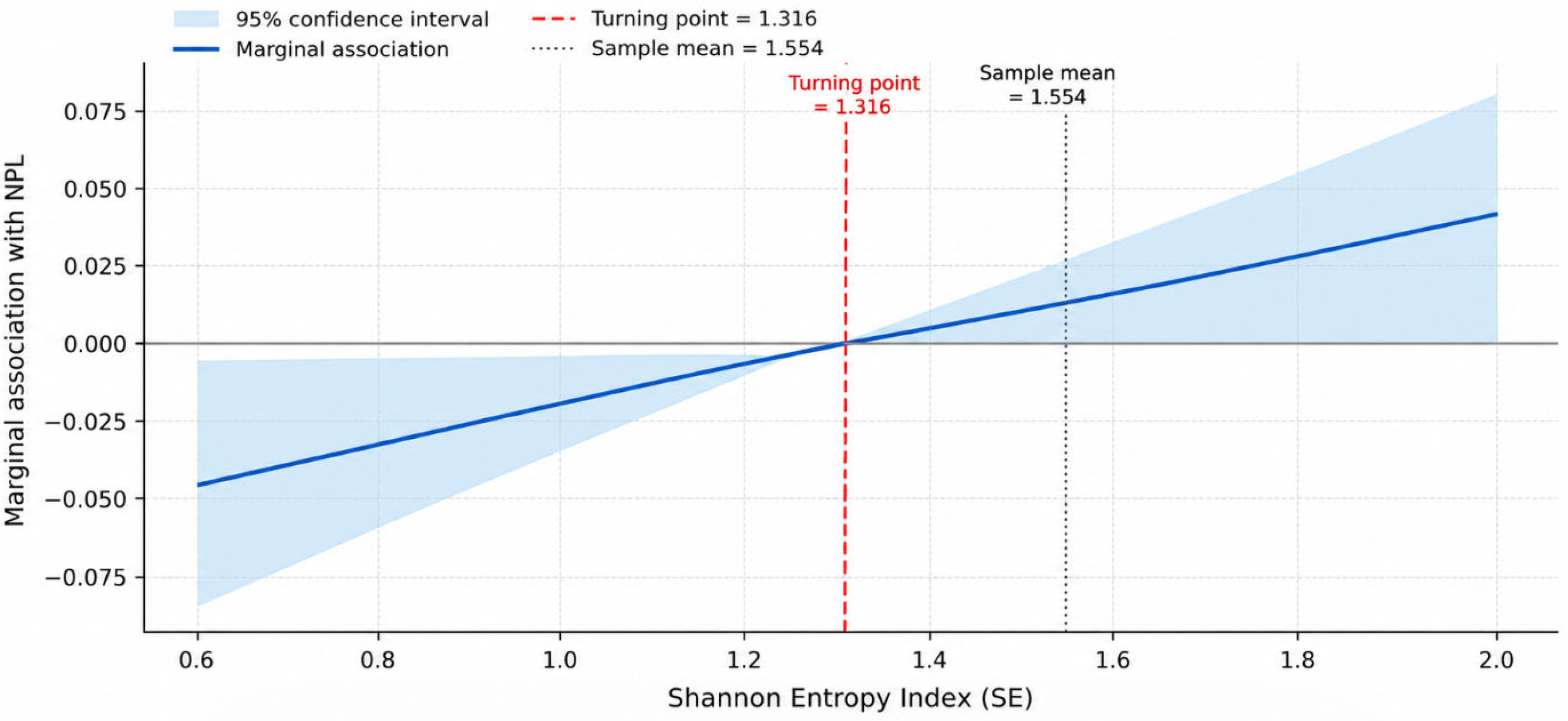
Figure 1 reports the estimated marginal association of SE with NPL across the observed range. The point estimate becomes positive above the turning point, but uncertainty must be considered. At the sample mean of SE (1.5536), the marginal point estimate is approximately 0.0145; the mean exceeding the turning point does not establish that most banks or bank-year observations have a statistically significant positive marginal association.

The insignificant FE and RE coefficients and the marginal 10% significance in GMM show that the nonlinear result is specification-sensitive. The positive CAP coefficient in the static models, contrary to its expected sign, may reflect defensive capitalization or reverse causality, whereby banks with higher risk hold more capital; this explanation is tentative. INF is positive in GMM but not statistically significant at the 10% level (β = 0.0653, p = 0.106).

The remaining GMM controls—SIZE, CAP, CRG, ROE, GDP, and INF—are statistically insignificant at conventional levels. Consequently, the discussion does not characterize inflation as a statistically established determinant in the preferred GMM specification.

4.3. Formal Shape Assessment and Robustness

Following Lind and Mehlum (2010), the slopes of the estimated relationship are evaluated at the lower and upper bounds of the observed SE range. At the lower bound (SE = 0.5842), the estimated slope is −0.0446 (standard error = 0.0204; two-sided p = 0.048), whereas at the upper bound (SE = 1.9739), it is 0.0401 (standard error = 0.0212; two-sided p = 0.081). Thus, the slope is negative at the lower bound and positive at the upper bound, with both estimates statistically significant at the 10% level. These results support the presence of a U-shaped association over the observed range, although they are based on separate boundary-slope tests rather than the overall Lind–Mehlum test statistic.

Normalized entropy produces an algebraically identical fitted model because SE_norm = SE/ln(10); it improves scale comparability but is not an independent robustness test. In contrast, HHI-based diversification retains the negative-linear/positive-quadratic sign pattern but neither term is significant, and its implied turning point (1.2458) lies outside the feasible range of DIV_HHI, which is at most 0.9 for ten sectors. The nonlinear finding is therefore sensitive to the diversification measure.

Bias-corrected LSDV estimates based on 1000 bootstrap replications provide supportive small-N evidence (Bruno, 2005). With Arellano–Bond initialization, SE is −0.0324 (SE = 0.0157; p = 0.039) and SE² is 0.0137 (SE = 0.00578; p = 0.018); with Blundell–Bond initialization, the corresponding estimates are −0.0321 (SE = 0.0172; p = 0.061) and 0.0137 (SE = 0.00629; p = 0.030). The implied turning points are 1.1808 (95% CI: 0.9146–1.4470) and 1.1769 (95% CI: 0.8818–1.4720), respectively, and both confidence intervals lie within the observed entropy range. Because a formal joint U-test was not obtained after LSDVC, these estimates are interpreted as supporting the negative-linear/positive-quadratic pattern rather than independently proving a U-shape over the full data range.

The distributional comparison shows that 163 of 182 dynamic-sample bank-year observations (89.56%) lie above the System GMM turning point of 1.3159; 13 of 14 banks also have a full-period mean SE above that value. These counts describe where the sample lies relative to a model-dependent threshold. They do not demonstrate that every observation above the threshold has a statistically significant positive marginal effect, that individual banks are over-diversified, or that further diversification causally raises NPLs.

The conditional turning point is best interpreted as a sample- and model-specific feature. Sector-only dispersion may fail to diversify common collateral, related-party, geographic, and macroeconomic exposures. Banks with broader portfolios may also differ systematically in monitoring capacity and risk appetite, which the available data do not fully measure.

The LSDVC estimates also show that credit growth and ROE are negatively associated with NPL, whereas inflation has a positive association. The negative coefficient of credit growth may reflect a short-term denominator effect, as newly expanded lending increases total loans before potential credit deterioration becomes observable (Foos et al., 2010). The negative association between ROE and NPL is consistent with the view that more profitable banks may possess stronger screening, monitoring, and loss-absorption capacity. Meanwhile, the positive inflation coefficient suggests that rising input costs, declining real income, and higher debt-servicing burdens may weaken borrowers’ repayment capacity.

Influence, leave-one-bank-out, ownership, size, pandemic-exclusion, year-effects, alternative risk-proxy, and flexible spline analyses could not be completed consistently with the available dataset and archived output. Their absence limits robustness. Future work should prioritize these tests with a larger bank sample and harmonized information on provisions, VAMC exposures, restructured loans, collateral, and borrower concentration.

Overall, the evidence challenges an unconditional maximization view of diversification but does not establish a normative optimum. The practical message is to evaluate sector concentration jointly with underwriting expertise, monitoring capacity, and correlations among underlying risk drivers.

To examine whether the nonlinear result is sensitive to the measurement of diversification, the model is re-estimated using normalized entropy and HHI-based diversification. The results are presented in

Table 5. Alternative diversification measures (two-step System GMM).

Variables and Statistics	Raw Entropy	Normalized Entropy	HHI-Based Diversification
NPLt−1	0.650 ***	0.650 ***	0.721 ***
	(0.154)	(0.154)	(0.101)
Diversification	−0.0803 *	−0.1848 *	−0.0924
	(0.0378)	(0.0869)	(0.172)
Diversification2	0.0305 *	0.1617 *	0.0741
	(0.0149)	(0.0789)	(0.141)
Conditional turning point	1.3159	0.5715	1.2458
Observed range	[0.5842, 1.9739]	[0.2537, 0.8573]	[0.2279, 0.8415]
Turning point within observed range	Yes	Yes	No
Observations	182	182	182
Number of banks	14	14	14

Notes: Normalized entropy is calculated as $SE/\mathrm{l}\mathrm{n}\left(10\right)$ and therefore represents a deterministic rescaling of raw entropy rather than an independent robustness test. HHI-based diversification is calculated as $1-HHI$. Its estimated turning point lies outside both the observed and theoretically feasible ranges. Standard errors are reported in parentheses. ***, and * indicate statistical significance at the 1%, and 10% levels, respectively. Source: Authors’ calculations.

.

Normalizing the Shannon Entropy Index changes the scale of the coefficients and turning point but leaves the fitted relationship and statistical inference unchanged. This result is expected because normalized entropy is a deterministic transformation of the original index. By contrast, the coefficients obtained using HHI-based diversification are statistically insignificant, and the implied turning point lies outside the observed range. Thus, the evidence of nonlinearity is sensitive to the diversification measure employed.

Because opposite signs on the linear and quadratic terms are not sufficient to establish a U-shaped relationship, the slopes are evaluated at the lower and upper bounds of the observed entropy range.

Table 6. Boundary slopes and conditional turning point.

Test Quantity	SE Value	Estimate	Standard Error	Test Result or Interval
Slope at the lower bound	0.5842	−0.0446	0.0204	$t=-2.18$; two-sided $p=0.048$
Slope at the upper bound	1.9739	0.0401	0.0212	$t=1.89$; two-sided $p=0.081$
Conditional turning point	—	1.3159	0.0485	95% CI: [1.2209, 1.4109]

Notes: The boundary slopes are calculated from the coefficient vector of the two-step System GMM model. The estimates display the negative lower-bound and positive upper-bound slopes required for a U-shaped relationship. However, these boundary calculations are not presented as a completed overall Lind–Mehlum U-test. Source: Authors’ calculations.

reports the boundary-slope estimates and the conditional turning point.

The estimated slope is negative and statistically significant at the lower bound, whereas it is positive and significant at the 10% level at the upper bound. The conditional turning point lies within the observed SE range. These results support a U-shaped association, although the inference is based on separate boundary-slope tests rather than the overall Lind–Mehlum test statistic.

Given the small number of banks in the sample, bias-corrected LSDV models are estimated as an additional check on the System GMM results.

Table 7. System GMM and bias-corrected LSDV estimates.

Variables and Statistics	System GMM	LSDVC–AB	LSDVC–BB
NPLt−1	0.650 ***	0.365 ***	0.377 ***
	(0.154)	(0.0470)	(0.0486)
SE	−0.0803 *	−0.0324 **	−0.0321 *
	(0.0378)	(0.0157)	(0.0172)
SE2	0.0305 *	0.0137 **	0.0137 **
	(0.0149)	(0.00578)	(0.00629)
SIZE	0.00148	0.00144	0.00150
	(0.00142)	(0.000939)	(0.00102)
CAP	0.00812	0.0187	0.0152
	(0.0382)	(0.0248)	(0.0270)
CRG	−0.00817	−0.00969 ***	−0.00994 ***
	(0.0136)	(0.00339)	(0.00365)
ROE	−0.0285	−0.0369 ***	−0.0365 ***
	(0.0211)	(0.0110)	(0.0119)
GDP	0.0269	0.0247	0.0246
	(0.0189)	(0.0248)	(0.0267)
INF	0.0653	0.0951 ***	0.0933 ***
	(0.0376)	(0.0327)	(0.0354)
Conditional turning point	1.3159	1.1808	1.1769
Turning-point 95% CI	[1.2209, 1.4109]	[0.9146, 1.4470]	[0.8818, 1.4720]
Observations	182	182	182
Number of banks	14	14	14

Notes: AAB and BB denote Arellano–Bond and Blundell–Bond initialization, respectively. LSDVC standard errors are obtained from 1000 bootstrap replications. LSDVC corrects dynamic fixed-effects bias in a small panel but does not, by itself, resolve the potential endogeneity of diversification. Standard errors are reported in parentheses. ***, **, and * indicate statistical significance at the 1%, 5%, and 10% levels, respectively. Source: Authors’ calculations.

compares the System GMM estimates with the LSDVC models initialized by the Arellano–Bond and Blundell–Bond estimators.

Both LSDVC specifications retain the negative coefficient on SE and the positive coefficient on SE². The corresponding turning points and their confidence intervals lie within the observed entropy range. The similarity of the coefficient patterns provides additional support for the nonlinear relationship in a small-panel setting, although LSDVC does not independently address the potential endogeneity of diversification.

To provide a descriptive assessment of the sample’s position relative to the System GMM turning point, bank-year observations and bank-level mean entropy values are classified as being below or above the estimated threshold. The results are reported in

Table 8. Sample distribution around the System GMM turning point.

Level of Comparison	At or Below 1.3159	Above 1.3159	Total	Share Above
Bank-year observations in the dynamic sample	19	163	182	89.56%
Banks classified by mean SE	1	13	14	92.86%

Notes: The bank-year classification is based on the 182 observations included in the dynamic System GMM model. The first observation of each bank is excluded because lagged NPL is unavailable. The bank-level classification compares each bank’s mean SE over 2012–2025 with the estimated turning point of 1.3159. These figures describe the sample distribution around a model-dependent turning point and do not establish that individual banks are over-diversified or experience statistically significant adverse marginal effects. Source: Authors’ calculations.

.

Most bank-year observations and bank-level mean entropy values lie above the estimated turning point. This distribution suggests that the upward-sloping segment of the estimated relationship is empirically relevant to a substantial part of the sample. However, exceeding the turning point does not necessarily imply that an individual bank is over-diversified or that its marginal effect is statistically significant.

Overall, the robustness analyses provide qualified support for a U-shaped association between sectoral loan diversification and reported NPLs. The System GMM and LSDVC estimates produce consistent coefficient patterns, with the estimated turning points located within the observed entropy range. However, the HHI-based specification does not yield statistically significant results. Taken together, the findings suggest that the association between sectoral diversification and credit risk varies with the degree of diversification and is captured more clearly by entropy-based measures than by HHI-based diversification.

5. Conclusions

This study examines the nonlinear association between sectoral loan diversification and reported NPLs in 14 Vietnamese commercial banks over 2012–2025. It combines a parsimonious quadratic specification with conventional panel estimators, two-step System GMM, alternative diversification measures, and bias-corrected LSDV estimates.

The findings provide qualified evidence of a U-shaped association between sectoral loan diversification and reported credit risk. Diversification appears to reduce NPLs at lower levels, while its marginal benefit diminishes and may reverse as banks expand into a broader range of sectors. However, the strength of this relationship varies across estimators and diversification measures. The estimated turning point should therefore be viewed as sample- and model-specific rather than as a universal optimal level.

These findings suggest that diversification should be managed in conjunction with banks’ sectoral expertise and risk-management capacity. Banks should consider not only the distribution of lending across sectors but also the underlying correlations among borrowers, collateral, and economic activities. For supervisors, sectoral concentration indicators can complement existing large-exposure regulations by supporting more comprehensive monitoring of credit concentration and internal risk governance.

Several limitations qualify the findings. The sample contains only 14 disclosure-consistent banks, creating finite-sample and selection concerns. System GMM relies on large-N asymptotics, and its diagnostic tests have low power here. Sector definitions require harmonization and sectoral entropy does not capture borrower, collateral, geographic, maturity, or related-party concentration. Reported NPLs exclude off-balance-sheet exposures and cannot be consistently adjusted for VAMC special bonds or restructured loans. Reverse causality and omitted variables may remain. Finally, the quadratic functional form and turning point are model-dependent, and the evidence is sensitive to the diversification measure. These limitations motivate larger samples, alternative risk proxies, flexible nonlinear specifications, and richer supervisory data.

References

1. Acharya, V. V., Hasan, I., & Saunders, A. (2006). Should banks be diversified? Evidence from individual bank loan portfolios. The Journal of Business, 79(3), 1355–1412. [Google Scholar] [CrossRef] [Scilit]
2. Arellano, M., & Bover, O. (1995). Another look at the instrumental variable estimation of error-components models. Journal of Econometrics, 68(1), 29–51. [Google Scholar] [CrossRef] [Scilit]
3. Basel Committee on Banking Supervision. (2000). Principles for the management of credit risk. Bank for International Settlements. [Google Scholar]
4. Beck, R., Jakubík, P., & Piloiu, A. (2015). Key determinants of non-performing loans: New evidence from a global sample. Open Economies Review, 26(3), 525–550. [Google Scholar] [CrossRef] [Scilit]
5. Behr, A., Kamp, A., Memmel, C., & Pfingsten, A. (2007). Diversification and the banks’ risk-return-characteristics: Evidence from loan portfolios of German banks. Deutsche Bundesbank Discussion Paper, Series 2: Banking and Financial Studies, No. 05/2007. Deutsche Bundesbank. [Google Scholar]
6. Berger, A. N., & DeYoung, R. (1997). Problem loans and cost efficiency in commercial banks. Journal of Banking & Finance, 21(6), 849–870. [Google Scholar] [CrossRef] [Scilit]
7. Berger, A. N., & Udell, G. F. (2002). Small business credit availability and relationship lending: The importance of bank organisational structure. The Economic Journal, 112(477), F32–F53. [Google Scholar] [CrossRef] [Scilit]
8. Blundell, R., & Bond, S. (1998). Initial conditions and moment restrictions in dynamic panel data models. Journal of Econometrics, 87(1), 115–143. [Google Scholar] [CrossRef] [Scilit]
9. Bruno, G. S. F. (2005). Approximating the bias of the LSDV estimator for dynamic unbalanced panel data models. Economics Letters, 87(3), 361–366. [Google Scholar] [CrossRef] [Scilit]
10. Cerasi, V., & Daltung, S. (2000). The optimal size of a bank: Costs and benefits of diversification. European Economic Review, 44(9), 1701–1726. [Google Scholar] [CrossRef] [Scilit]
11. Diamond, D. W. (1984). Financial intermediation and delegated monitoring. The Review of Economic Studies, 51(3), 393–414. [Google Scholar] [CrossRef] [Scilit]
12. Elsas, R., Hackethal, A., & Holzhäuser, M. (2010). The anatomy of bank diversification. Journal of Banking & Finance, 34(6), 1274–1287. [Google Scholar] [CrossRef] [Scilit]
13. Foos, D., Norden, L., & Weber, M. (2010). Loan growth and riskiness: Evidence from individual banks. Journal of Banking & Finance, 34(12), 2929–2940. [Google Scholar] [CrossRef] [Scilit]
14. Hayden, E., Porath, D., & von Westernhagen, N. (2007). Does diversification improve the performance of German banks? Evidence from individual bank loan portfolios. Journal of Financial Services Research, 32(3), 123–140. [Google Scholar] [CrossRef] [Scilit]
15. Huynh, J., & Dang, V. D. (2022). Exploring the asymmetric effects of loan portfolio diversification on bank profitability. Journal of Economic Asymmetries, 26, e00250. [Google Scholar] [CrossRef] [Scilit]
16. International Monetary Fund. (2021). Global financial stability report: COVID-19, preemptive policies, and avoiding a new wave of financial instability. Available online: https://www.imf.org/en/Publications/GFSR/Issues/2021/04/06/global-financial-stability-report-april-2021 (accessed on 5 June 2026).
17. Kamp, A., Pfingsten, A., & Porath, D. (2005). Do banks diversify loan portfolios? A tentative answer based on individual bank loan portfolios. Discussion Paper Series 2: Banking and Financial Studies No. 03/2005. Deutsche Bundesbank. [Google Scholar]
18. Klein, N. (2013). Non-performing loans in CESEE: Determinants and impact on macroeconomic performance. IMF Working Paper 13/72. International Monetary Fund. [Google Scholar]
19. Lind, J. T., & Mehlum, H. (2010). With or without U? The appropriate test for a U-shaped relationship. Oxford Bulletin of Economics and Statistics, 72(1), 109–118. [Google Scholar] [CrossRef] [Scilit]
20. Louzis, D. P., Vouldis, A. T., & Metaxas, V. L. (2012). Macroeconomic and bank-specific determinants of non-performing loans in Greece: A comparative study of mortgage, business and consumer loan portfolios. Journal of Banking & Finance, 36(4), 1012–1027. [Google Scholar] [CrossRef] [Scilit]
21. Markowitz, H. (1952). Portfolio selection. The Journal of Finance, 7(1), 77–91. [Google Scholar] [CrossRef] [Scilit]
22. National Assembly of Vietnam. (2024). Law on credit institutions. No. 32/2024/QH15. National Assembly of Vietnam. [Google Scholar]
23. Nkusu, M. (2011). Nonperforming loans and macrofinancial vulnerabilities in advanced economies. IMF Working Paper No. 11/161. International Monetary Fund. [Google Scholar]
24. Roodman, D. (2009). How to do xtabond2: An introduction to difference and system GMM in Stata. The Stata Journal, 9(1), 86–136. [Google Scholar] [CrossRef] [Scilit]
25. Rossi, S. P. S., Schwaiger, M. S., & Winkler, G. (2009). How loan portfolio diversification affects risk, efficiency and capitalization: A managerial behavior model for Austrian banks. Journal of Banking & Finance, 33(12), 2218–2226. [Google Scholar] [CrossRef] [Scilit]
26. Shim, J. (2019). Loan portfolio diversification, market structure and bank stability. Journal of Banking & Finance, 104, 103–115. [Google Scholar] [CrossRef] [Scilit]
27. Stiglitz, J. E., & Weiss, A. (1981). Credit rationing in markets with imperfect information. American Economic Review, 71(3), 393–410. [Google Scholar]
28. Tabak, B. M., Fazio, D. M., & Cajueiro, D. O. (2011). The effects of loan portfolio concentration on Brazilian banks’ return and risk. Journal of Banking & Finance, 35(11), 3065–3076. [Google Scholar] [CrossRef] [Scilit]
29. Windmeijer, F. (2005). A finite sample correction for the variance of linear efficient two-step GMM estimators. Journal of Econometrics, 126(1), 25–51. [Google Scholar] [CrossRef] [Scilit]
30. Winton, A. (1999). Don’t put all your eggs in one basket? Diversification and specialization in lending. Center for Financial Institutions Working Paper No. 00-16. Wharton School, University of Pennsylvania. [Google Scholar] [CrossRef] [Scilit]
Figure 1. Estimated marginal association between sectoral diversification and reported NPL. Notes: The line shows ∂NPL/∂SE = β1 + 2β2SE from the two-step System GMM model. The shaded area is the 95% confidence interval derived from the reported covariance matrix. Vertical lines mark the conditional turning point and sample mean. Source: Authors’ calculation.
Ijfs 14 00250 g001