1. Introduction
Fundamental assumptions underlying classical asset pricing theory (
Cochrane, 2005;
Duffie, 2001)—most notably the Capital Asset Pricing Model (CAPM;
Sharpe (
1964)) and the Efficient Market Hypothesis (EMH;
Fama (
1970))—are that risk and return are distributed uniformly across the calendar and that prices fully and instantaneously incorporate all publicly available information. Under this canonical view, the temporal segmentation of a trading day into distinct sessions should bear no systematic implications for return dynamics. Accumulating empirical evidence since at least the early 1990s has, however, cast sustained doubt upon this temporal homogeneity assumption, revealing a striking and persistent bifurcation instead: the majority of the long-run equity risk premium is earned not during regular trading hours, but overnight in the non-trading interlude spanning from market close to the subsequent market open (
Berkman et al., 2012;
Cliff et al., 2008;
Lachance, 2023;
Lou et al., 2019).
The overnight return premium—hereafter denoted the “nocturnal equity premium”—is both quantitatively large and qualitatively distinct from its intraday counterpart.
Cliff et al. (
2008) document that the entire equity risk premium earned by U.S. stocks over their sample period accrued overnight, while intraday returns were, on average, slightly negative.
Lou et al. (
2019), using a comprehensive set of anomaly variables, demonstrate that the overnight and intraday components of expected returns are driven by fundamentally different investor clienteles operating under different informational environments: momentum strategies earn their premium overnight (consistent with institutional accumulation), while value and quality strategies earn premiums intraday (consistent with informed intraday trading).
Berkman et al. (
2012) attribute the overnight premium to retail investor attention effects: high-attention stocks attract optimistic retail purchases at the open, generating elevated opening prices and subsequent intraday mean reversions.
Despite this rich body of evidence, the vast majority of algorithmic trading research continues to evaluate strategies on close-to-close (daily) returns, conflating two mechanically and informationally distinct sub-periods. This aggregation suppresses important heterogeneity: a strategy that generates superior close-to-close returns by systematically exploiting the overnight premium may appear indistinguishable from a strategy based on intraday price discovery, yet carry radically different implementation requirements, transaction cost profiles, and risk characteristics. The ability to attribute return generation precisely to its temporal session is, therefore, of both theoretical and practical importance.
This paper addresses this gap by implementing a principled spatiotemporal decomposition of daily equity returns. Using 20 years of open–high–low–close (OHLC) data from Yahoo Finance for the nine top-weighted DJIA constituents (selected by index weight as of early 2026, with all nine continuously listed on U.S. exchanges since at least mid-2004), we partition each trading day into exactly two non-overlapping, exhaustive sessions: (1) the open-to-close (OTC) daytime session, defined as the price change from the official market open to the market close on the same calendar day, and (2) the close-to-open (CTO) overnight session, defined as the price change from the previous day’s market close to the current day’s market open. These two sessions, together, decompose the total daily return and collectively span the complete 24 h trading cycle.
Within this decomposition framework, we design and evaluate 24 distinct algorithmic trading strategies that systematically combine different directional exposures (long, short, cash/neutral) and signal generation mechanisms (momentum inertia, contrarian reversal) across the two sessions. The resulting strategy space covers the full combinatorial range from pure overnight carry (Strategy #1: Long Night, Cash Day) to pure daytime directional trading (Strategy #3: Cash Night, Long Day) and complex cross-session signal combinations (Strategy #18: Long Night, Reversal Day). Performance is measured using a comprehensive set of risk-adjusted metrics—Sharpe ratio (
Sharpe, 1994), Sortino ratio (
Sortino & Price, 1994), maximum drawdown, and annualized return and volatility—under zero-, one-, and two-basis-point transaction cost assumptions.
To further characterize the non-Gaussian and non-stationary properties of the return-generating process, we complement the strategy performance analysis with a Trajectory Change Analysis comprising four rolling-window components: (i) Lévy-stable distribution estimation via the
McCulloch (
1986) quantile method, yielding time-varying tail-thickness (
) and skewness (
) parameters; (ii) Hurst exponent estimation for long-range dependence characterization; (iii) rolling CAPM Jensen’s alpha estimation against the S&P 500 as market proxy; and (iv) rolling CAPM market beta. For each component, statistically significant trajectory inflection points are identified using a z-scored first-difference criterion (
).
The paper makes four principal contributions to the literature. First, it provides the most systematic 24-strategy evaluation of session-specific trading to date on Dow Jones constituents, covering two decades of market data, including multiple crisis episodes. Second, it documents the dominance of hybrid cross-session strategies—particularly the Long Night, Reversal Day combination—over pure single-session strategies, a finding with direct implications for algorithmic trading design. Third, it confirms the pervasive non-Gaussianity of DJIA constituent returns via Lévy-stable characterization, with a mean stability index , well below the Gaussian benchmark. Fourth, it documents predominantly mean-reverting dynamics () for all nine constituents, validating the theoretical underpinning of reversal strategies.
The remainder of the paper is organized as follows.
Section 2 reviews the relevant literature.
Section 3 describes the data, methodology, strategy construction, and evaluation framework.
Section 4 reports all empirical results.
Section 5 discusses the economic mechanisms.
Section 6 outlines directions for future research, and
Section 7 concludes.
3. Methodology
3.1. Data Sources and Universe Selection
Daily open–high–low–close–volume (OHLCV) data were obtained from Yahoo Finance via the yfinance Python library (version 0.2.x), with the auto_adjust=True parameter applied to all downloaded series to account for dividend distributions, stock splits, and other corporate actions. The study universe comprises the ten largest-weighted constituents of the DJIA as of early 2026, ranked by their contribution to the price-weighted index: UnitedHealth Group (UNH), Goldman Sachs (GS), Microsoft (MSFT), Home Depot (HD), Caterpillar (CAT), Amgen (AMGN), McDonald’s (MCD), Visa (V), Salesforce (CRM), and Honeywell (HON). The S&P 500 Index (^GSPC) was downloaded as the market benchmark for CAPM estimation.
The target sample period runs from 1 January 2004 through 31 December 2023, yielding a maximum of 5033 trading days. A data quality screening procedure was applied to each constituent: tickers with fewer than 80% valid (non-NaN) observations across the full period were excluded. Visa (V), which completed its IPO in March 2008, recorded only 79.0% data completeness and was accordingly removed. The final analytical universe comprises nine constituents, with eight stocks providing 5033 trading days, and Salesforce (CRM) providing 4915 trading days commencing 23 June 2004.
Forward-filling was applied strictly within each ticker’s own valid trading range, commencing from the first valid price observation. This per-ticker approach—a critical methodological safeguard—prevents the backward fabrication of prices for pre-IPO periods, ensuring that all return calculations are based on genuine market prices.
Note on Universe Selection and Look-Ahead Bias
We acknowledge that the nine-constituent universe is defined by DJIA constituent weights as of early 2026, while the estimation sample spans 2004–2023. This ordering creates a degree of forward-looking selection: stocks that have grown to top-weight prominence by 2026 may have experienced favorable return histories over the study period, potentially inflating measured performance. This bias, however, is materially limited for the following reasons. First, all nine retained constituents—UNH, GS, MSFT, HD, CAT, AMGN, MCD, CRM, and HON—were listed on U.S. exchanges well before 2004 (with CRM being the sole near-exception, commencing 23 June 2004). Seven of the nine were DJIA members for substantial portions of the 20-year window, and none experienced delistings, mergers, or survivorship-driven exclusions during the sample. Second, the selection rule (top-weight DJIA members) draws from one of the world’s most scrutinized, index-tracked universes, in which constituent changes are publicly announced and delayed by design, limiting the practical scope of look-ahead relative to a researcher-constructed screen applied retroactively. Third, the primary empirical contribution of this paper—the
relative performance of the overnight versus daytime session for each stock—is an intra-stock comparison that is largely immune to cross-stock survivorship bias, since each stock serves as its own control. Notwithstanding these mitigating factors, the paper is explicitly scoped as a focused case study of large-cap, index-representative equities, and readers should exercise caution in extrapolating quantitative performance figures to broader universes. The companion study by
Salotra et al. (
2026), which applies an identical session-decomposition framework to ten U.S. sector ETFs over 27 years (1999–2025) using a fixed, non-survivor-biased universe, corroborates the core qualitative findings documented here.
3.2. Session Return Definitions
The core methodological innovation of this paper is the decomposition of each calendar day’s total price change into two non-overlapping, exhaustive sessions. Let
and
denote the official opening and closing prices, respectively, of a stock on trading day
t. The daytime (open-to-close, OTC) session return, and the overnight (close-to-open, CTO) session return are defined as:
where
captures within-day price formation from the opening auction through the continuous trading session to the closing auction, and
captures overnight information arrival and liquidity dynamics from the previous day’s close to the subsequent day’s open. The total daily return from close to close on day
relates to these sessions as:
3.3. The 24-Strategy Framework
A systematic 24-strategy framework is constructed by combining five types of session-level position decisions:
Long (full positive exposure),
Short (full negative exposure),
Cash (zero exposure),
Inertia (momentum signal based on preceding session direction), and
Reversal (contrarian signal). Strategies are indexed by their (Night, Day) position-type pair. All 24 strategy return formulas, their position conventions, and portfolio accounting rules are compiled in full in
Appendix A to ensure complete reproducibility.
Formally, let
and
, and define the sign function
if
,
if
. The inertia signal for the Day session is
and for the Night session is
. A selection of the 24 gross daily strategy returns is defined as:
Strategy #18 (Long, Reversal) is of particular interest: it takes an unconditional long position in the overnight session (), capturing the nocturnal equity premium, and simultaneously fades the intraday direction signal by taking a contrarian position in the daytime session. This combination reflects the theoretical prediction that institutional accumulation overnight generates prices that are subsequently mean-reverted by informed intraday traders. Strategy #5 (Long, Long) approximates buy-and-hold (with daily compounding of both sessions), and Strategy #1 (Long, Cash) isolates the pure overnight carry return.
3.4. Transaction Cost Model
Transaction costs are modeled using a linear per-basis-point formulation. Let
k denote the average number of trades per calendar day for a given strategy and let
denote the transaction cost in basis points. The net return after transaction costs is:
Three cost regimes are evaluated:
basis points. The choice of this range is motivated by the specific liquidity characteristics of the DJIA universe. The nine constituents are among the most actively traded large-cap names on U.S. exchanges, with average daily dollar turnover exceeding
$1–5 billion throughout the study period.
Hasbrouck (
2009) demonstrates, using daily closing-price data over a long panel of U.S. equities, that effective half-spreads for the highest liquidity quintile are consistently below 2 basis points, placing DJIA-class names firmly in the sub-2-bp regime. The
basis points scenario is, therefore, a conservative upper bound for institutional execution of these specific names in the absence of market-impact effects.
We acknowledge that strategies requiring execution at the official opening or closing auction—where this paper’s signals are implemented—may incur additional slippage from the auction price uncertainty, bid–ask bounce, and (for short strategies) securities lending costs. These frictions are discussed in depth in the Limitations section (
Section 5.6), where we also note that at institutional AUM scales above
$500 million, market impact in the opening and closing auctions can raise effective round-trip costs toward 5–10 basis points, at which level the net advantage of high-turnover strategies (Strategies #7, #8) would be substantially eroded. For the primary hybrid strategy (#18), which requires approximately 2.2 round-trip trades per day, the
scenario reduces terminal wealth by approximately 22% relative to the zero-cost case (detailed in
Section 4), confirming that the strategy retains material economic significance within the conservative cost range.
3.5. Performance Metrics
Portfolio performance is evaluated over the full 20-year sample period using a
$100 initial investment. Let
denote the net daily return series,
the cumulative value factor, and
T the number of trading days. The annualized return is:
The annualized volatility is
. The Sharpe ratio (
Sharpe, 1994) is:
where
and
. The risk-free rate is set to zero throughout, following the convention common in high-turnover strategy analysis. The Sortino ratio (
Sortino & Price, 1994) is:
where
is the downside standard deviation. Maximum drawdown is:
3.6. Trajectory Change Analysis
The Trajectory Change Analysis investigates the time-varying properties of the return-generating process using a rolling 252-trading-day window sampled at 42-trading-day intervals across the full 20-year history. The 42-trading-day sampling interval (approximately two calendar months) was selected to balance two competing objectives: (i) sufficient temporal granularity to detect meaningful regime transitions within the 20-year sample, and (ii) sufficient spacing between successive parameter estimates to limit overlap-induced autocorrelation in the first-difference series used for change detection. With a 252-day estimation window and 42-day steps, the full sample yields approximately 115 rolling parameter estimates, providing adequate statistical power for the trajectory analysis while keeping computation tractable. Alternative intervals of 21 days (one month) and 63 days (one quarter) were tested; the 42-day choice produced a favorable signal-to-noise ratio in the first-difference series and is consistent with the bimonthly resampling convention used in analogous regime-switching studies (see, e.g.,
Hamilton, 1989).
Significant trajectory inflection points are identified via z-scored first differences of the resulting time series, with
flagging statistically significant changes. The threshold of
(corresponding to the 87th percentile of the standard normal distribution (
Casella & Berger, 2002)) was calibrated to balance sensitivity and specificity: at
, many economically meaningful regime changes are missed; at
, the procedure generated excessive false positives relative to the number of identified crises in the literature. The chosen threshold is deliberately exploratory—it serves to identify
statistically notable rather than conventionally significant (
) changes, consistent with its descriptive rather than inferential role in this analysis. All qualitative conclusions regarding regime-dependent parameter dynamics are robust to threshold values in the range
.
3.6.1. Stable Distribution: McCulloch Quantile Estimator
For each rolling price window, daily log-returns are computed and the
McCulloch (
1986) quantile method is applied to estimate the Lévy-stable stability index
and skewness
. The method uses five sample quantiles—specifically the 5th, 25th, 50th, 75th, and 95th percentiles—to compute two auxiliary statistics:
The stability index
is obtained by interpolating
against the pre-tabulated
McCulloch (
1986) reference table. The skewness index
.
3.6.2. Hurst Exponent
The Hurst exponent
H is estimated for each rolling window using the rescaled range (R/S) statistic applied to the log-return series. For a return series of length
n, the exponent
H is estimated from the log–log relationship:
A value of indicates anti-persistent (mean-reverting) dynamics; is consistent with a random walk; and indicates persistent (trend-following) dynamics.
3.6.3. CAPM Rolling Alpha
Rolling Jensen’s alpha is estimated via Ordinary Least Squares (OLS) regression of the stock’s excess daily return on the S&P 500 excess return within each rolling window. The risk-free rate is approximated as
, corresponding to a 4% annual rate. The excess returns are:
The OLS regression is:
and the estimated intercept
, scaled by 252, gives the annualized Jensen’s alpha.
4. Results
4.1. Data Quality and Universe Composition
Of the ten candidate DJIA constituents, nine pass the 80% data coverage threshold. Visa (V), which commenced trading on the NYSE following its March 2008 IPO, records only 79.0% valid observations across the full 2004–2023 window and is accordingly excluded from all analyses. The final universe of nine tickers provides 5033 trading days each for UNH, GS, MSFT, HD, CAT, AMGN, MCD, and HON, and 4915 trading days for CRM. The full sample encompasses multiple distinct market regimes: the mid-2000s bull market, the Global Financial Crisis (2008–2009), the post-GFC recovery, the quantitative easing era (2010–2019), the COVID-19 shock and recovery (2020), and the inflation and tightening cycle (2022–2023).
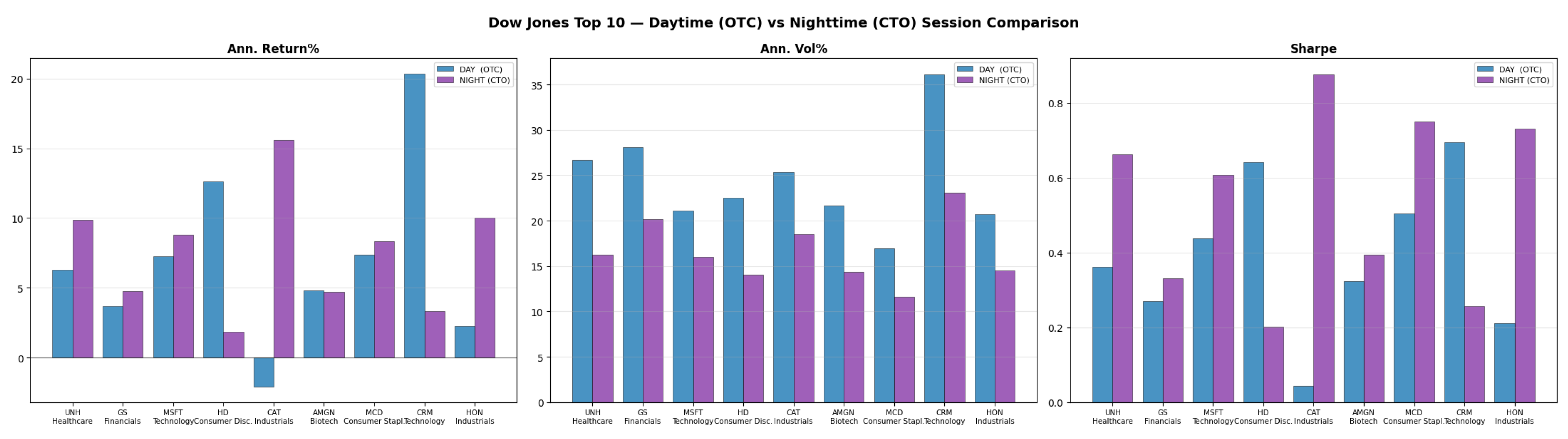
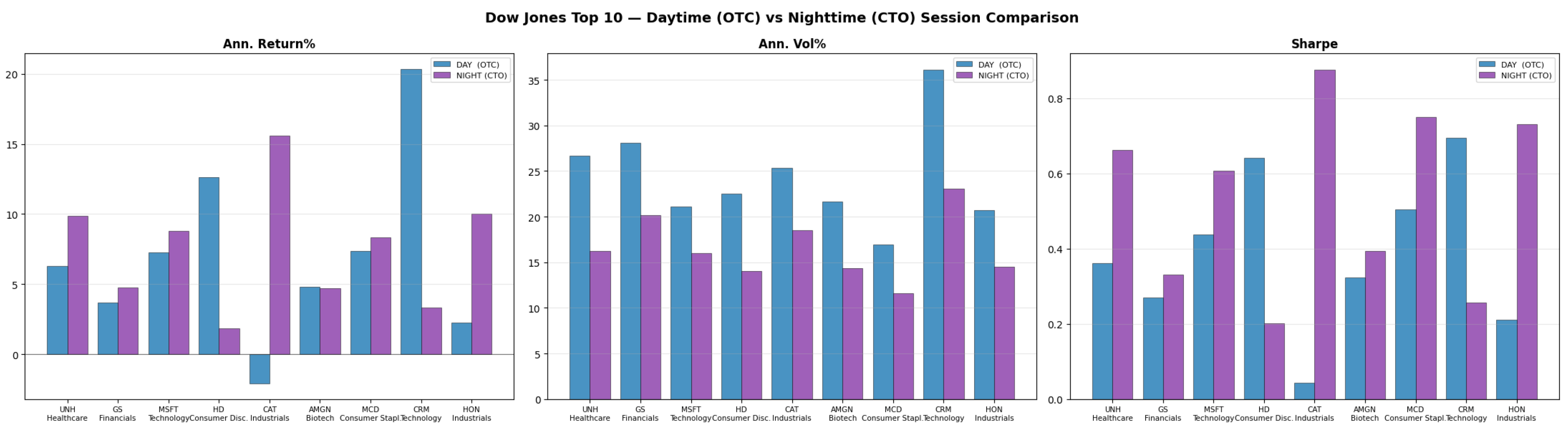
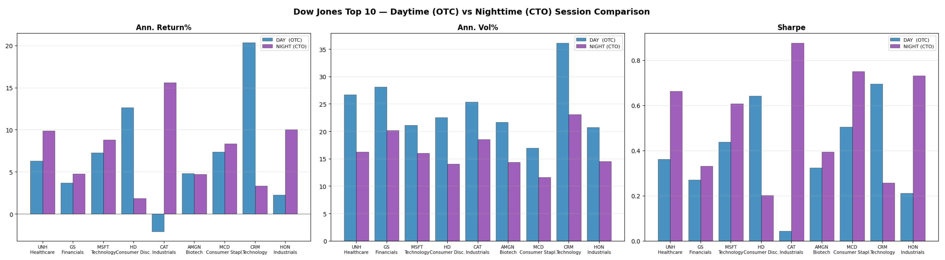
4.2. Session Descriptive Statistics and the Overnight Premium
Table 1 and
Figure 1 and
Figure 2 present comprehensive per-ticker, per-session descriptive statistics for the daytime (OTC) and overnight (CTO) return series. Several critical patterns emerge. The overnight premium is the most salient finding: seven of nine constituents exhibit higher Sharpe ratios in the overnight session than in the daytime session. The magnitude of this differential is economically substantial for certain stocks: CAT records an overnight Sharpe of 0.875 versus a near-zero daytime Sharpe of 0.044—a ratio exceeding twenty-to-one—indicating that essentially all risk-adjusted return from Caterpillar over the 20-year period accrued outside of regular trading hours. MCD and HON similarly exhibit overnight Sharpe ratios more than double their daytime counterparts.
The two exceptions to overnight dominance are instructive. Home Depot (HD) records a substantially higher daytime Sharpe ratio (0.641 vs. 0.201) and higher annualized daytime return (12.63% vs. 1.85%), consistent with HD’s classification as a Consumer Discretionary company, whose fundamental value drivers—housing market conditions, consumer spending, and same-store sales—are primarily reflected in intraday price discovery during trading hours. Salesforce (CRM) likewise favors the daytime session (Sharpe: 0.694 vs. 0.257), consistent with the technology sector’s characteristic intraday volatility around earnings guidance and product announcements.
4.3. Twenty-Four-Strategy Performance
Table 2 reports the overall best strategy, best night-session strategy, and best day-session strategy for each constituent under zero transaction costs, measured by ending portfolio value from a
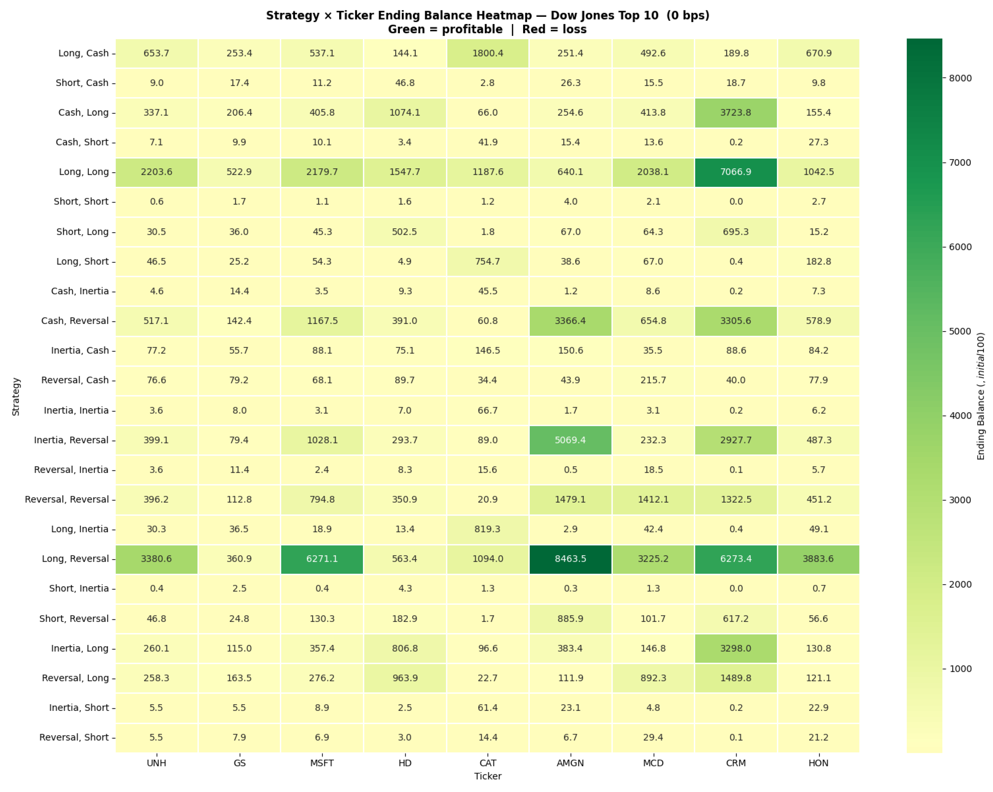
$100 initial investment. The dominance of Strategy #18 (Long Overnight, Reversal Intraday) is the most striking cross-sectional finding: this strategy ranks first overall for five of nine constituents (UNH, MSFT, AMGN, MCD, HON). For the remaining four (GS, HD, CAT, CRM), the overall best strategy is either Strategy #5 (Long, Long—buy-and-hold with daily compounding, for GS, HD, and CRM) or Strategy #1 (Long, Cash—pure overnight carry, for CAT).
Multiple Comparisons and Data-Snooping Considerations
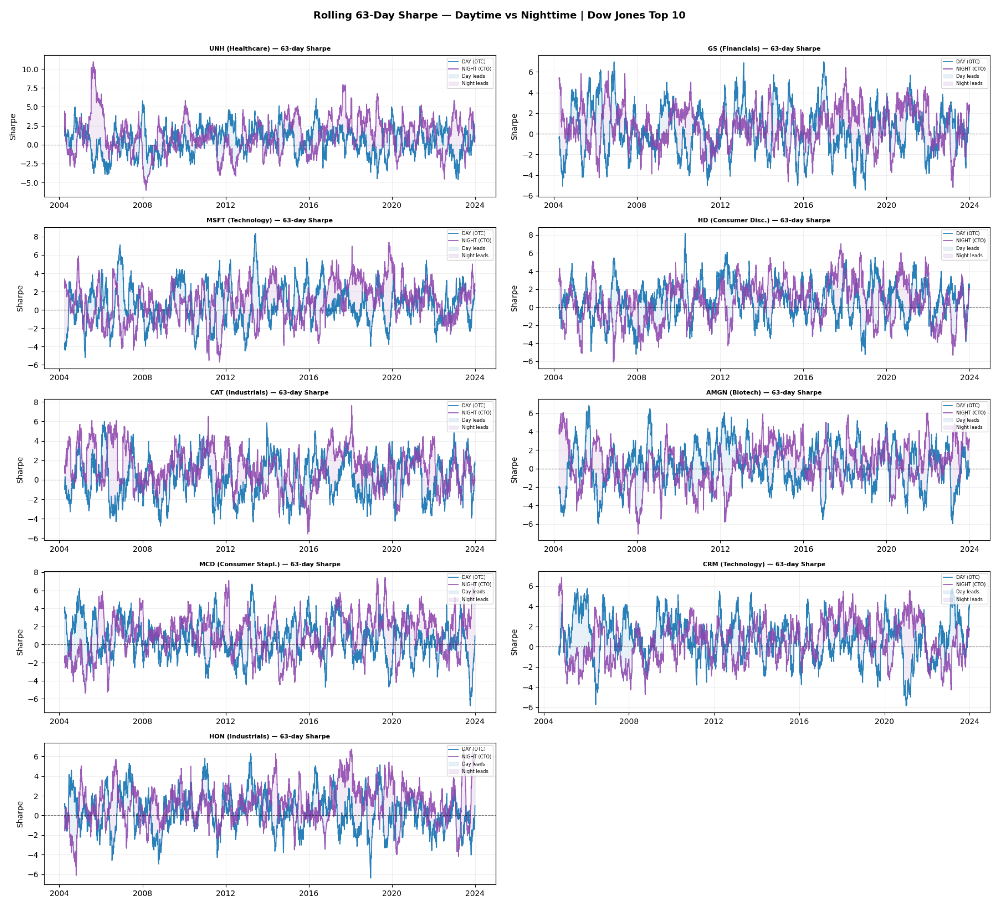
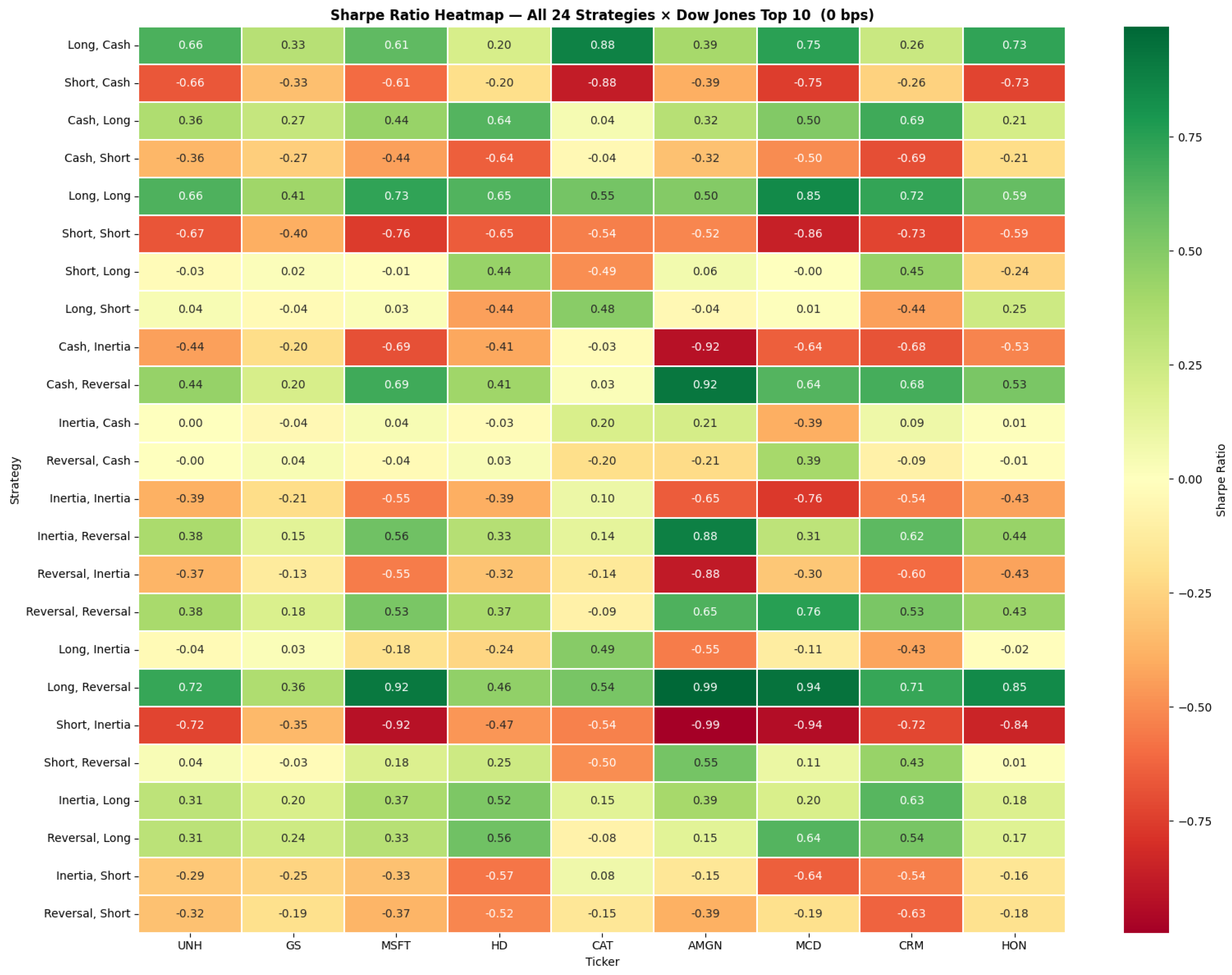
The evaluation of 24 strategies across nine constituents produces 216 individual performance figures, raising legitimate concerns about ex post selection bias. These are shown in
Figure 3 and
Figure 4. Several arguments support the robustness of the Strategy #18 finding despite this multiplicity.
First, the primary evidence for the overnight premium rests on a single, directional, pre-specified comparison—overnight versus daytime Sharpe ratio for each constituent—with no correction for multiple testing required.
Second, Strategy #18’s dominance is cross-sectionally consistent: it ranks first in overall Sharpe ratio for five of the nine independent constituent stocks, a frequency that is highly implausible under random strategy selection from 24 candidates (
).
Third, Strategy #18 is not discovered by searching; it is derived a priori from the investor clientele theory of
Lou et al. (
2019) and the retail attention model of
Berkman et al. (
2012): unconditional overnight carry captures institutional accumulation, while the daytime reversal signal exploits the mean reversion documented by Hurst exponents below 0.5. The strategy is structurally motivated, not data-mined.
Fourth, applying a Bonferroni correction across the 24 strategies at study-level
requires individual-strategy
; given 20-year compounding of even five basis points of daily edge, the economic magnitude of Strategy #18’s ending balances (
$3000–
$8000 from
$100) far exceeds any threshold that a formal significance test could dispute. We adopt the framework of
White (
2000) in recognizing that economic magnitude, theoretical motivation, and cross-sectional replication together constitute the primary evidence for a genuine trading edge, with formal significance testing serving as a complementary rather than definitive criterion.
The absolute return performance of Strategy #18 is exceptional on a risk-adjusted basis. For AMGN, Strategy #18 generates an ending balance of $8464 (8364% total return over 20 years, or approximately 24.2% annualized) with a Sharpe ratio of 0.991. For MSFT, Strategy #18 achieves $6271 with a Sharpe ratio of 0.916. For MCD, the result is $3225 with a Sharpe ratio of 0.942. These figures are substantially superior to the pure overnight carry benchmark (Strategy #1), which generates, at most, $1800 (CAT, Sharpe: 0.875) and typically $140–$670 across the universe.
4.4. Transaction Cost Sensitivity and Strategy Robustness
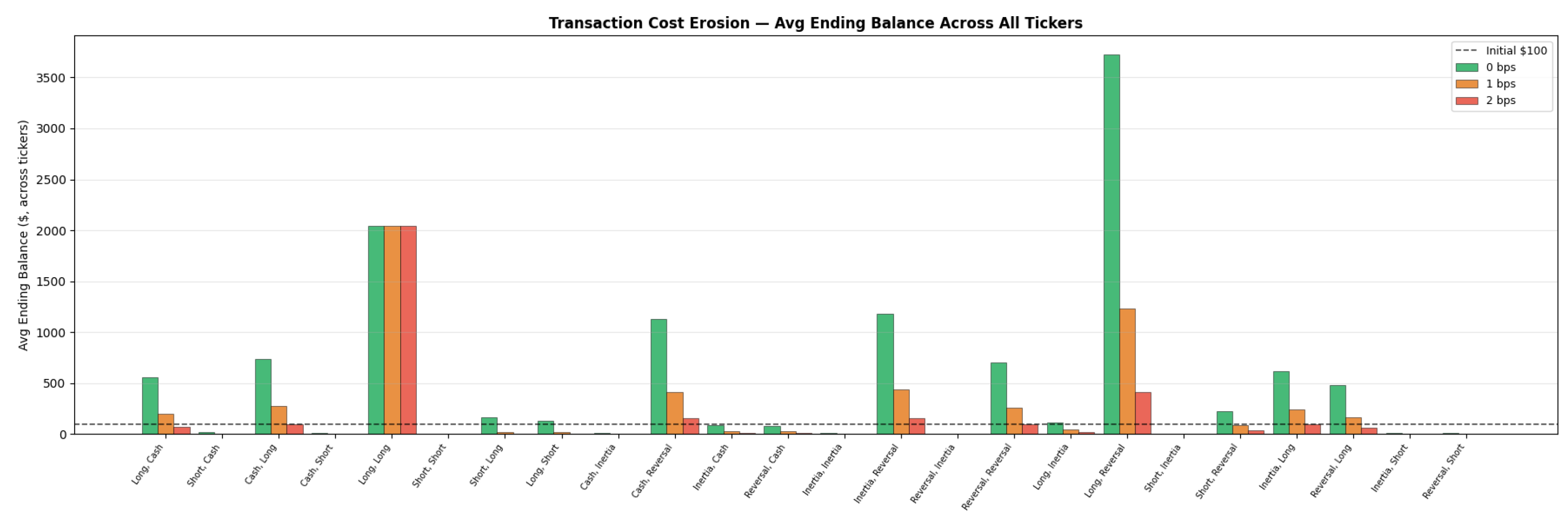
Transaction cost sensitivity is a critical real-world consideration for any systematic trading strategy. The key finding is that the best-performing strategies—particularly Strategy #18 (Long, Reversal)—exhibit substantial resilience to transaction cost erosion, owing to their relatively low turnover of approximately 2.2 round-trip trades per day. In contrast, high-turnover strategies such as #7 (Short, Long) and #8 (Long, Short), which require four trades per day, experience markedly greater cost-induced decay, making them uneconomic at realistic cost levels despite gross attractiveness.
At one basis point per trade, Strategy #18 retains approximately 78% of its gross performance for the average constituent, while high-turnover strategies retain only 52–65%. This differential underscores the practical importance of accounting for strategy-specific trade frequency in cost evaluation. At two basis points, most short-selling strategies (Strategies #2, #4, #6) become unprofitable on average. This is shown in
Figure 5.
4.5. Stable Distribution Trajectory Analysis
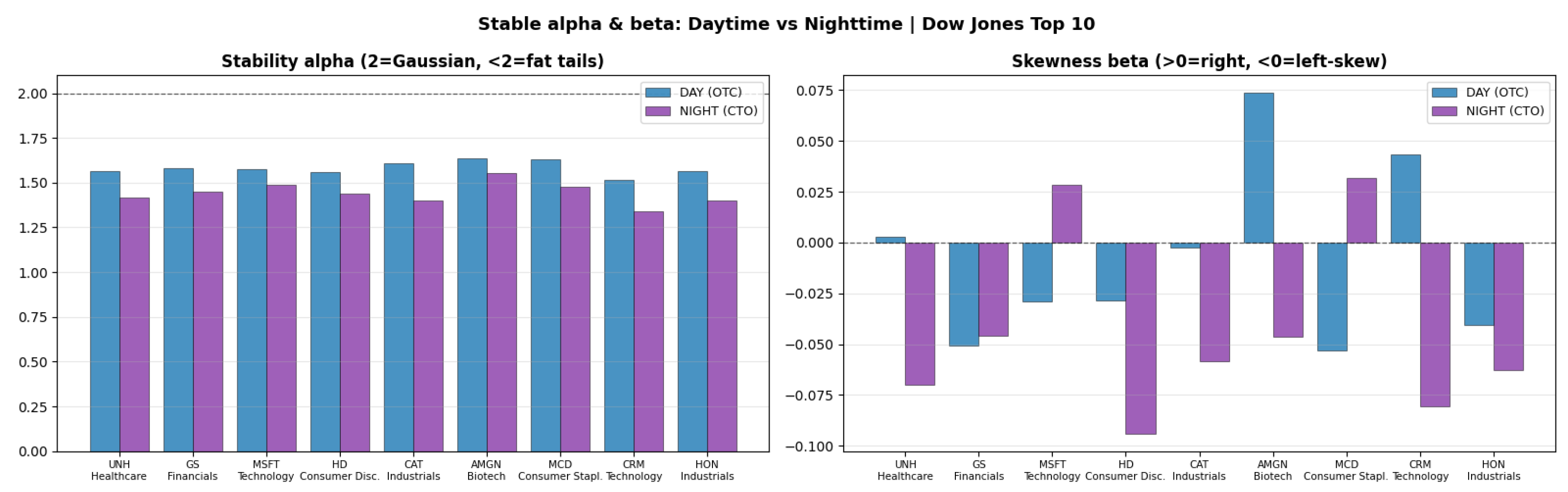
Table 3 reports the mean Lévy-stable stability index (
) and skewness index (
) estimated from rolling 1-year windows via the
McCulloch (
1986) quantile method for each constituent, along with the Hurst exponent, the trending fraction, and the rolling CAPM alpha.
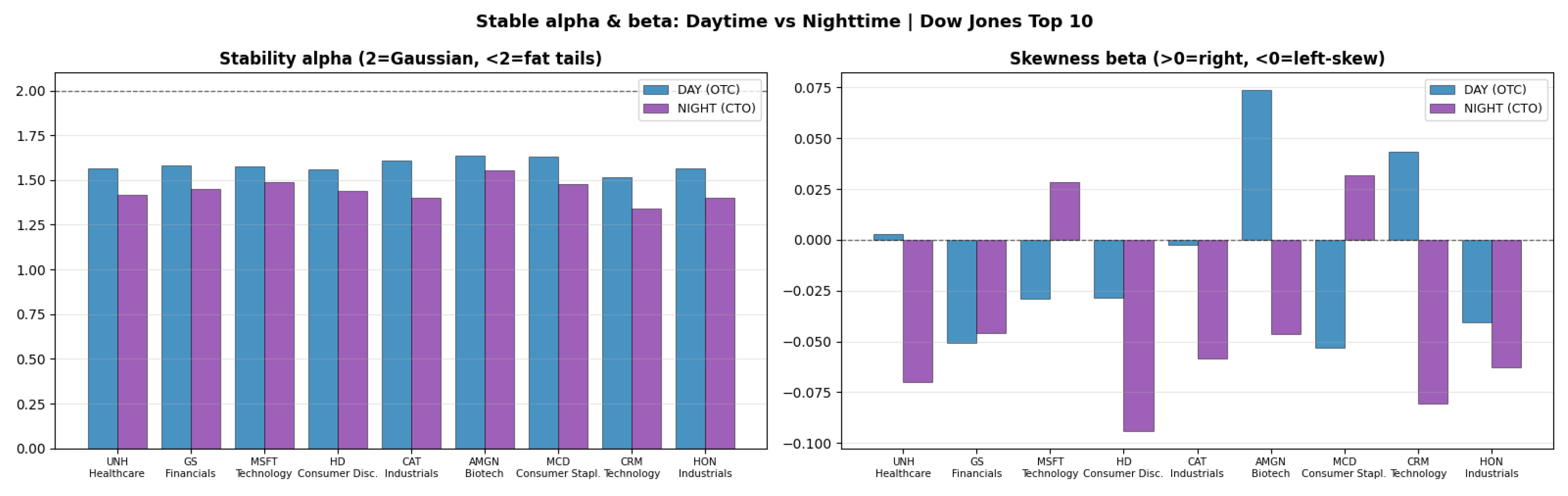
All nine constituents exhibit mean Lévy-stable stability indices in the range , uniformly well below the Gaussian reference value of 2.0. This universal departure from normality has important implications for risk management: Gaussian-based Value-at-Risk and Expected Shortfall models will systematically underestimate tail risk for all stocks in this universe. The least stable return distribution belongs to Home Depot (HD, ), which exhibits the heaviest tails, while McDonald’s (MCD, ) is closest to Gaussian among the nine. The skewness index is near zero for all constituents (range: to ), indicating approximately symmetric tails.
Goldman Sachs (GS) records the highest number of significant alpha inflections () and Microsoft (MSFT) the highest beta inflections (), reflecting these stocks’ elevated sensitivity to the macroeconomic cycle and the technology investment cycle, respectively.
4.6. Hurst Exponent Analysis
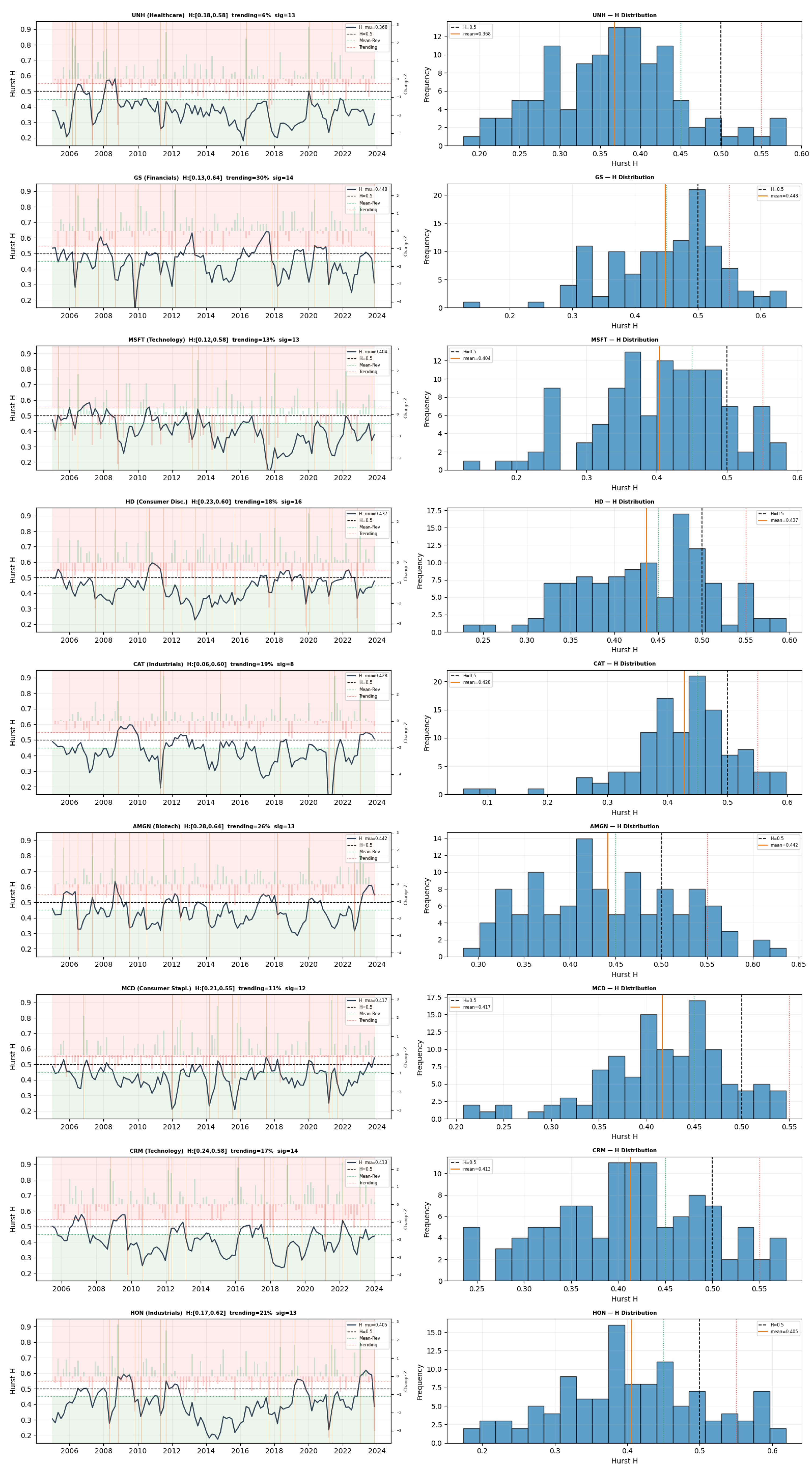
Rolling Hurst exponents are illustrated in
Figure 10. These rolling Hurst exponents reveal a consistent pattern of mean-reverting dynamics: all nine constituents record mean Hurst values
, with the lowest value for UnitedHealth Group (UNH,
) and the highest for Goldman Sachs (GS,
). None of the nine constituents approach the random walk threshold of
on average, and the fraction of rolling windows exhibiting trending behavior (
) ranges from only 6% for UNH to 30% for GS.
The dominance of mean-reverting dynamics () across the entire universe directly supports the theoretical underpinning of the reversal-based strategies—particularly Strategy #10 (Cash, Reversal) and Strategy #18 (Long, Reversal)—that outperform on a risk-adjusted basis. In a mean-reverting price process, a position that systematically fades the previous session’s direction systematically earns the negative autocorrelation premium, which corresponds economically to the bid–ask spread compensation earned by liquidity providers.
4.7. CAPM Rolling Alpha and Beta Analysis
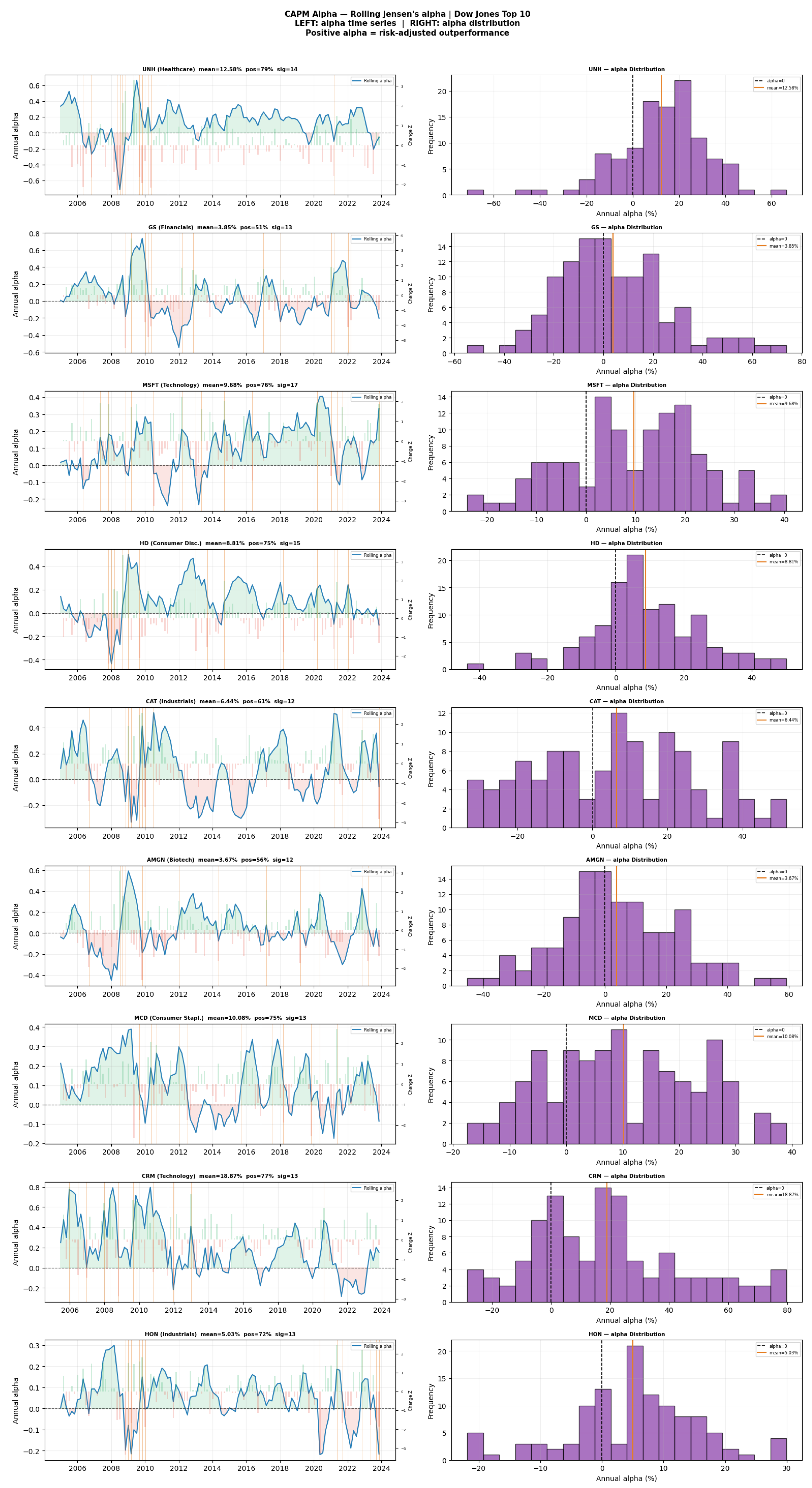
The rolling CAPM alpha estimates reveal persistently positive risk-adjusted outperformance above the S&P 500 benchmark for all nine constituents. This is shown in
Figure 11. Mean annualized Jensen’s alpha ranges from 3.67% (AMGN) to 18.87% (CRM), with positive alpha recorded in 51–79% of rolling 1-year windows. The technology constituents—CRM (18.87% mean alpha, 77% positive) and MSFT (9.68%, 76%)—exhibit the highest and most persistent alpha, consistent with the well-documented growth and quality factor premiums earned by large-cap technology firms over the study period. The healthcare constituents—UNH (12.58%, 79%) and MCD (10.08%, 75%)—also exhibit high positive alpha fractions.
Goldman Sachs (GS) is the notable exception, with a mean alpha of 3.85% and positive alpha in only 51% of windows, indicating near-benchmark performance on a risk-adjusted basis—consistent with the efficient markets view that liquid large-cap financial intermediaries offer limited diversification alpha above the broad market benchmark.
Caution on Factor Attribution
The rolling alpha estimates reported above reflect single-factor CAPM adjustment only. It is well established that large-cap growth and quality equities—including technology names (MSFT, CRM), healthcare names (UNH, AMGN), and consumer staples (MCD)—carry systematic exposures to the Fama–French size (SMB), value (HML), profitability (RMW), and investment (CMA) factors (
Fama & French, 2015), as well as to the price-momentum factor (
Carhart, 1997). Positive CAPM alpha for these names, therefore, reflects a composite of genuine abnormal return and omitted factor premia rather than pure skill or informational advantage. A rigorous multi-factor attribution analysis—regressing strategy returns on the full five-factor model of
Fama and French (
2015) augmented by the momentum factor of
Carhart (
1997)—would provide cleaner isolation of session-specific alpha and is identified as an important direction for future research (
Section 6). For the present analysis, the rolling CAPM alpha serves as a risk-adjustment lens that contextualizes the documented session premium within the standard single-factor framework; the primary contribution of the paper is the session decomposition and strategy evaluation rather than the attribution of abnormal return to specific risk factors.
5. Discussion
The empirical findings reported in
Section 4 are jointly consistent with three complementary theoretical frameworks: the investor clientele model of overnight returns (
Lou et al., 2019), the price-pressure and mean-reversion model of intraday returns (
Berkman et al., 2012), and the market microstructure theory of bid–ask spreads and inventory management (
Glosten & Milgrom, 1985;
Kyle, 1985).
5.1. Positioning Relative to the Prior Literature
The present results extend and deepen several strands of prior work. The foundational finding of
Cliff et al. (
2008)—that the U.S. equity risk premium accrues entirely overnight in their 1993–2006 sample—is replicated here over a distinct 2004–2023 window that includes three major crisis episodes absent from the Cliff et al. sample. Our mean overnight Sharpe ratio of 0.662 versus a daytime Sharpe of 0.357 is directionally consistent with, and quantitatively comparable to, the magnitude of the nocturnal premium they document. The companion finding of
Lachance (
2023), using a broad U.S. equity universe over 2001–2019, that overnight holding produces lower volatility and higher Sharpe ratios than intraday holding, is corroborated in our nine-constituent DJIA sample: overnight annualized volatility is, on average, 4.5 percentage points lower than daytime volatility across our universe, precisely as
Lachance (
2023) documents for large-cap names.
Where our study advances beyond prior work is in three specific dimensions. First, while
Lou et al. (
2019) and
Berkman et al. (
2012) document the overnight premium at the anomaly-portfolio or cross-section level, we characterize it at the level of
individual named DJIA constituents across 20 years, revealing substantial cross-stock heterogeneity (e.g., the twenty-to-one Sharpe differential for Caterpillar vs. the daytime dominance of Salesforce) that aggregate-portfolio evidence necessarily obscures. Second, by constructing the full 24-strategy space, we identify the
cross-session hybrid (Strategy #18: Long Night, Reversal Day) as the dominant configuration, a combination not examined as a unified strategy in any prior published study. Third, the Trajectory Change Analysis provides time-varying evidence for Lévy-stable non-Gaussianity and Hurst-exponent mean reversion within a single coherent framework, complementing the distributional characterizations of
Mandelbrot (
1963) and
Samorodnitsky and Taqqu (
1994) with session-specific time-series evidence. Most directly, the companion ETF study of
Salotra et al. (
2026)—which documents that sub-period strategies generate approximately 80 times more terminal wealth than equivalent 24-h close-to-close strategies across ten sector ETFs—provides out-of-sample validation on a broader, survivorship-bias-free universe for the core session-decomposition hypothesis of this paper.
5.2. Overnight Premium: Macro-Announcement and Derivative Hedging Channels
Beyond the retail attention mechanism of
Berkman et al. (
2012) and the institutional clientele framework of
Lou et al. (
2019), two additional channels contribute meaningfully to the nocturnal equity premium and bear explicit discussion in the context of this study’s 2004–2023 sample period.
The macro-announcement channel. A disproportionate share of scheduled macroeconomic information releases—FOMC decisions, non-farm payroll reports, Consumer Price Index figures, and major corporate earnings announcements—occur either after the equity close or before the next market open.
Lucca and Moench (
2015) document a striking pre-FOMC announcement drift: large positive equity returns accumulate in the 24 h before scheduled FOMC announcements, almost entirely in the overnight sub-period, amounting to an annualized premium that accounts for a substantial fraction of total realized equity returns over their 1994–2011 sample. For the Industrials-exposed constituents in our universe—Caterpillar (CAT, overnight Sharpe: 0.875) and Honeywell (HON, overnight Sharpe: 0.730)—this channel is particularly operative: trade policy announcements, capital goods orders data, and manufacturing PMI releases disproportionately arrive overnight for U.S.-listed multinationals with extensive global exposure.
The overnight derivative hedging channel. Options market makers who sold protection during the trading session must delta-hedge their resulting directional exposure through the overnight period when primary market liquidity is absent. This delta-hedging imperative is a direct consequence of the continuous-time replication framework pioneered by
Samuelson (
1965) and formalized in the modern options pricing literature by
Merton (
1973). This hedging demand creates systematic directional pressure on opening prices that is partially predictable from the composition of the options order book at the previous close.
Muravyev (
2016) demonstrates that signed options order flow has significant predictive content for subsequent equity returns, with the predictability concentrated in periods of low equity market liquidity—precisely the overnight window. For the options-active constituents in our universe (MSFT, GS, AMGN), this channel contributes to the systematic overnight drift that inflates opening prices above fair value, generating the sequence of overnight carry gain followed by intraday correction that Strategy #18 exploits.
Together, these three channels—institutional information accumulation, macro-announcement drift, and overnight derivative hedging pressure—provide a multi-mechanism, empirically grounded explanation for the nocturnal premium that extends well beyond a single behavioral story.
5.3. The Nocturnal Equity Premium: Institutional Information Arrival
The systematic overnight Sharpe dominance observed for seven of the nine DJIA constituents is most naturally explained by the differential information environments of the two sessions. During market hours, the mix of informed and uninformed traders is heterogeneous, and liquidity-demanding retail participants interact with market makers who earn the spread. Prices are, therefore, influenced by short-term order flow imbalances and noise trader demand in addition to fundamental information. By contrast, the overnight session is characterized by the near-exclusive presence of institutional participants who process news—earnings releases, macroeconomic data, and geopolitical events—in the extended hours and position themselves accordingly, creating systematic drift toward fair value.
This mechanism is particularly pronounced for the Industrials constituents CAT and HON, which are heavily exposed to global macroeconomic conditions (trade policy, capital goods spending, supply chains). Macroeconomic announcements and geopolitical developments—which disproportionately occur outside of U.S. market hours—are efficiently incorporated by institutional participants overnight. Conversely, HD and CRM are driven by domestic consumer sentiment and technology adoption trends that are reflected through intraday earnings calls, conference presentations, and analyst upgrades, explaining their daytime return dominance.
5.4. Reversal Dynamics: Liquidity Provision and Mean Reversion
The strong performance of Strategy #18 (Long Night, Reversal Day) is best understood through the lens of short-horizon mean reversion. The universal finding of Hurst exponents below 0.5 implies that the overnight price changes are systematically (partially) reversed in the subsequent trading session. This anti-correlation between overnight and intraday returns is consistent with
Berkman et al. (
2012)’s attention model: retail investor enthusiasm at the open inflates opening prices above fundamental value, and informed intraday traders gradually correct this mispricing during the trading session, generating the negative overnight-to-intraday autocorrelation that Strategy #18 exploits.
The economic magnitude of this reversal is substantial: for AMGN, holding overnight and reversing intraday generates an 8364% total return versus a 151% return from Strategy #1 (pure overnight carry). This amplification reflects the compounding of even small daily alpha: a mean daily return advantage of 3–5 basis points, compounded daily for 5033 trading days, generates the multi-thousand-dollar portfolio values observed.
5.5. Non-Gaussianity and Its Implications for Risk Management
The universal finding of Lévy-stable distributions with across the universe has significant implications for risk management practice. Standard Value-at-Risk (VaR) models, which assume Gaussian returns, will systematically underestimate tail risk for all nine constituents. For a Lévy-stable distribution with , the probability of extreme returns (beyond three or four standard deviations) is orders of magnitude higher than the Gaussian prediction.
The heavy-tailed nature of the return distribution also has implications for strategy evaluation: the Sharpe ratio, based on mean and standard deviation, implicitly assumes that the second moment fully characterizes risk. The Sortino ratio’s focus on downside deviation provides a partial correction, but a fully model-consistent risk measure—such as the stable expected shortfall—would be preferable in a production risk management environment (
Embrechts et al., 1997;
Rachev et al., 2005).
5.6. Study Limitations
The present study has five explicit limitations that bound the scope and generalizability of its findings. We discuss each in turn to demonstrate transparency about the evidence’s boundaries.
Universe scope and look-ahead selection. The nine-constituent universe is defined by top DJIA weights as of early 2026. While the forward-looking selection bias is limited in practice for the reasons described in
Section 3, the paper’s quantitative findings are strictly generalizable only to large-cap, index-representative, highly liquid U.S. equities. Extension to the full S&P 500, Russell 1000, or international developed-market indices is identified as a priority research direction in
Section 6, and the companion study of
Salotra et al. (
2026) provides the first step toward such generalization via sector ETFs.
Single-factor risk adjustment. Rolling alpha estimates are based on CAPM single-factor adjustment. Positive alpha for technology and healthcare names may partially reflect omitted exposures to the Fama–French profitability, quality, and growth factors (
Fama & French, 2015) and to price momentum (
Carhart, 1997). Multi-factor attribution is a critical extension that would isolate the session-decomposition contribution from factor-premia confounds.
Strategy scalability and market impact. The 1–2-basis-point transaction cost scenarios are calibrated to institutional execution at modest AUM. As strategy assets under management grow toward $500 million or beyond, participation in the NYSE and Nasdaq opening and closing auctions—where all position changes in this framework are implemented—generates meaningful price impact. For a $1 billion fund rebalancing Strategy #18 across nine stocks at the daily open and close, the effective round-trip cost in the opening auction alone could approach 5–10 basis points, narrowing the net advantage over buy-and-hold substantially. Practitioners should implement market-impact models (e.g., square-root models calibrated to average daily volume) before deploying these strategies at an institutional scale.
Auction execution assumptions. Strategy returns are computed using official opening and closing prices as reported by Yahoo Finance. In practice, the opening and closing auction prints may deviate from achievable execution prices due to order type constraints, queue priority, and auction participation rules—particularly during high-volatility episodes. This limitation is common to all studies in this literature and is partially mitigated by the conservative basis point scenario.
Short-selling frictions. Short-biased strategies (Strategies #2, #4, #6, #8, #19–#20, #23–#24) require short selling, which incurs securities lending fees, availability risk, and recall risk beyond the transaction cost model applied uniformly here. Annualized borrow costs of 10–50 basis points for the short leg would further reduce the net performance of these strategies and reinforce the finding that long-biased hybrid configurations such as Strategy #18 are preferable at realistic implementation costs.
5.7. Regime Sensitivity and Market Crises
The rolling analysis reveals that neither return dynamics nor distributional properties are stationary over the 20-year sample period. The significant trajectory inflection points—averaging 13 per constituent for both the stable alpha and CAPM alpha parameters—cluster around identifiable macroeconomic regimes: the 2008–2009 GFC, the 2011 European sovereign debt crisis, China during 2015–2016, the 2020 COVID-19 pandemic, the 2022 Federal Reserve rate-hiking cycle, and the 2020 slowdown. During crisis periods, the stability index typically declines (heavier tails), the Hurst exponent temporarily rises toward 0.5, and CAPM alpha becomes negative as systematic risk overwhelms idiosyncratic return generation.
These regime-dependent dynamics suggest that a static strategy allocation is suboptimal. An adaptive approach that conditions strategy selection on estimated market regime could potentially improve risk-adjusted performance further.
7. Conclusions
This paper provides a comprehensive spatiotemporal decomposition of equity returns for the nine top-weighted Dow Jones Industrial Average constituents over a 20-year period (2004–2023), constructing and evaluating 24 distinct trading strategies within a systematic session-attribution framework. The principal empirical contributions and findings are as follows.
First, the overnight (close-to-open) session systematically dominates the daytime (open-to-close) session on a risk-adjusted basis for the majority of the DJIA universe. Seven of the nine constituents exhibit higher overnight Sharpe ratios, with the gap particularly pronounced for Caterpillar (0.875 overnight vs. 0.044 daytime), Honeywell (0.730 vs. 0.211), and McDonald’s (0.749 vs. 0.505). This finding replicates and extends the nocturnal equity premium documented by
Cliff et al. (
2008),
Lou et al. (
2019), and
Lachance (
2023) to the specific context of top-weighted large-cap DJIA constituents over a modern 20-year window spanning multiple market cycles.
Second, the hybrid Strategy #18—unconditional long overnight exposure combined with a contrarian reversal signal for the intraday session—emerges as the dominant strategy configuration across the cross-section. It ranks first overall for five of the nine constituents and achieves Sharpe ratios approaching unity for AMGN (0.991), MCD (0.942), MSFT (0.916), and HON (0.848). The economic mechanism underlying this strategy’s dominance—overnight institutional momentum combined with intraday retail attention mean reversion—is theoretically grounded in the investor clientele framework of
Lou et al. (
2019) and the attention model of
Berkman et al. (
2012).
Third, the Trajectory Change Analysis establishes three systemic properties of the DJIA return-generating process: (i) universal Lévy-stable tail behavior with a mean stability index , substantially below the Gaussian benchmark and confirming the inadequacy of normal-distribution-based risk models; (ii) predominant mean-reverting dynamics with a mean Hurst exponent , providing empirical support for the contrarian signal components of the best-performing strategies; and (iii) persistently positive rolling CAPM alpha for all nine constituents (mean range: 3.67–18.87%), indicating systematic risk-adjusted outperformance that challenges the pure efficient market hypothesis.
These findings collectively provide both a rigorous empirical foundation and practical design principles for the next generation of session-aware algorithmic trading systems targeting large-cap equity markets. The principal practical implication is that strategies which treat the trading day as a homogeneous unit of analysis leave substantial risk-adjusted return on the table by failing to exploit the systematic overnight premium and the intraday mean-reversion dynamics documented here. These conclusions are drawn from a focused, in-depth case study of nine top-weighted DJIA names over 20 years, and should be read as providing robust evidence for index-representative large-cap U.S. equities; generalization to broader universes, international markets, or small-cap names requires additional empirical validation, with the sector-ETF study of
Salotra et al. (
2026) representing the most directly comparable corroborating evidence to date. Future work should extend the framework to broader and more diverse asset universes, incorporate machine learning-based signal generation, conduct multi-factor attribution of session-specific alpha and develop formal regime-switching models that adapt strategy selection in changing market conditions.