Article

Tail Risk Spillovers Between FinTech and Sustainability Sectors: Evidence from China Using Factor-Purged Quantile Connectedness

1
Shenzhen Key Laboratory of Organic Pollution Prevention and Control, School of Economics and Management, Harbin Institute of Technology, Shenzhen 518055, China
2
Department of Business Administration, University of Sahiwal, Sahiwal 57000, Punjab, Pakistan
3
College of Business Administration, Prince Sultan University, Riyadh 11586, Saudi Arabia
*
Authors to whom correspondence should be addressed.
Int. J. Financial Stud. 2025, 13(4), 218; https://doi.org/10.3390/ijfs13040218
Submission received: 9 September 2025 / Revised: 5 November 2025 / Accepted: 11 November 2025 / Published: 18 November 2025

Abstract

The rapid integration of FinTech and sustainability-oriented sectors is reshaping financial risk dynamics, particularly in emerging markets such as China. This study investigates tail-dependent spillovers among ten Chinese FinTech and sustainability-linked sectors from 2015–2024 using a factor-purged Quantile Vector Autoregression (QVAR) with generalized forecast error variance decompositions. By isolating idiosyncratic shocks, the framework uncovers how risk creation, transmission, and absorption vary across market states. Results show that (i) FinTech acts as a net transmitter of shocks in adverse (lower-tail) states, amplifying downside risk to clean energy and green innovations; (ii) policy-intensive sectors (environmental and atmospheric governance) switch roles across quantiles, revealing asymmetric regulatory spillovers; and (iii) diversification benefits compress in the tails, with cross-sector linkages intensifying during crises. These findings highlight the importance of quantile-specific stress testing for regulators and the design of state-contingent hedging strategies for portfolio managers.
JEL Classification:
C32; G11; G14; G18; Q42; Q58

1. Introduction

The accelerating interplay between financial technology (FinTech) and sustainability-oriented sectors is reshaping how risks are created, transmitted, and absorbed in modern economies. China offers a natural laboratory for studying the FinTech–sustainability nexus given the scale of digital finance, rapid ESG uptake, and an active green–finance policy mix. In this paper, we measure how tail risks propagate across FinTech and sustainability sectors in China by applying a factor-purged Quantile VAR model to daily sector indices (2015–2024). We find that FinTech is a major transmitter of extreme downside shocks to clean energy and green innovation sectors, policy-related sectors like environmental governance alternate between transmitting and absorbing shocks depending on the market state, and cross-sector diversification fails in the tails. Our objective is not to establish structural causality but to measure state-contingent risk propagation across FinTech and sustainability-linked sectors using quantile connectedness. By focusing on tail outcomes (e.g., the worst 10% of days), we capture dynamics that mean-based models would miss.
Recently digital financial infrastructure, green bond issuance, carbon governance, and technology-enabled public services have all expanded rapidly in China. These developments connect capital-intensive, policy-sensitive industries (such as clean energy, green finance, and environmental governance) with data and platform-driven verticals (intelligent transportation, digital healthcare). In this paper, “risk creation” refers to shocks originating in financing or policy nodes; “risk transmission” describes how those shocks spread through liquidity, regulation, or demand channels; and “risk absorption” captures sectors that predominantly receive shocks under specific market conditions. Capturing these state-contingent spillovers requires methods beyond mean-based models, which average away extremes. In the quantile FEVD framework, we interpret ‘risk creation’ as own-shock variance, ‘risk transmission’ as directional spillovers to other nodes, and ‘risk absorption’ as net-receiving contributions. This perspective aligns with recent work on tail connectedness (Ando et al., 2022; Choi, 2022; Shang & Hamori, 2024; Sun et al., 2024; Tiwari et al., 2022; M.-C. Wang et al., 2024).
Methodologically, we rely on quantile connectedness because mean-based VARs understate tail co-movements that matter for asset allocation, stress testing, and systemic oversight (Diebold & Yilmaz, 2012). The recent finance literature documents materially different networks at the extremes and time variation in spillovers that intensify during crises (Choi, 2022; M.-C. Wang et al., 2024). Our approach complements those studies by factor-purging common components before computing quantile FEVDs, sharpening inference on idiosyncratic shock propagation (e.g., platform- or policy-specific). While the approach does not deliver structural causality, it provides transparent, quantile-specific evidence on systemic linkages (Ando et al., 2022; Diebold & Yilmaz, 2014) (Ando et al., 2022; Chatziantoniou et al., 2021; Koop et al., 1996; Pesaran & Shin, 1998).
Anchored in this literature, we study daily Chinese stocks and bonds (January 2015–July 2024) spanning ten sustainability-linked sectors: FinTech, green finance, clean energy, green innovations, environmental governance (including atmospheric quality), water and water treatment, solid waste treatment, intelligent transportation, and digital healthcare. This broad yet policy-coherent system is theoretically connected by funding/liquidity channels (FinTech platforms, green credit/bond markets), regulatory spillovers (carbon/ESG rules, environmental governance), and technology/real-economy links (digital healthcare and transport platforms relying on financing and data rails). Modeling these sectors jointly allows us to: (i) assess whether FinTech behaves as a net transmitter of shocks to sustainability verticals in stress states (funding channel), (ii) evaluate policy-intensive nodes (e.g., environmental governance proxies) as state-dependent transmitters/absorbers, and (iii) gauge whether diversification benefits compress in tails when connectedness rises. Recent scholarship has deepened our understanding of green finance and systemic tail-risk transmission. Bolton and Kacperczyk (2021) highlight a growing “carbon premium” in asset pricing, underscoring investor sensitivity to climate risk exposures. Their findings support the notion that clean energy and carbon-intensive assets are priced differently under regulatory and investor pressure, aligning with our investigation into spillovers affecting green sectors. Similarly, Giglio et al. (2016) identify common systemic risk factors, laying a foundation for analyzing aggregate tail-risk propagation. Our use of factor-purged quantile connectedness builds on this approach by isolating idiosyncratic sectoral dynamics. We also relate our methodology to Tobias and Brunnermeier’s (2016) CoVaR framework, which models conditional value-at-risk to quantify systemic vulnerability in distress scenarios. The recent literature has increasingly highlighted the evolving role of FinTech in China’s financial system, particularly its implications for credit allocation, risk transmission, and systemic stability. Fang et al. (2023) demonstrate that FinTech-driven liquidity creation can enhance credit supply but also amplify risk exposure through changes in banks’ credit structures. Similarly, Zhang et al. (2021) and Tian et al. (2024) provide evidence that rapid FinTech expansion contributes to network contagion and tail-risk spillovers, reinforcing concerns about systemic vulnerability. While some studies, such as R. Wang et al. (2021) and Deng et al. (2021), find that FinTech can reduce bank risk-taking by increasing transparency and competitive discipline (Deng et al., 2021; R. Wang et al., 2021), others caution that digital lending platforms, particularly P2P lenders, can exacerbate liquidity shocks during downturns (Chen et al., 2020; Li et al., 2020). These findings are underscored by the real-world collapse of China’s P2P lending sector by 2020, which highlighted the sector’s potential to propagate instability. Collectively, these studies motivate a closer examination of FinTech’s role in transmitting tail risks to sustainability-linked sectors within China’s financial landscape. These works collectively situate our analysis within a robust and evolving literature on climate-related financial risk, state-dependent spillovers, and financial technology’s systemic implications. Fresh advances show that spillover structures in sustainable vs. conventional markets are strongly state-dependent and asymmetric. Using quantile connectedness, Karim (2025) documents that transmitters/receivers rotate across market states: traditional energy dominates in booms, while eco-indices and strategic minerals are more exposed to stress; robustness is validated with a QVAR check. These patterns imply that portfolio risk and policy transmission differ markedly in the lower vs. upper tails. Complementing this market-side view, Aharon et al. (2025) integrate climate policy uncertainty (CUI) with green/dirty assets and show that CUI is a net transmitter during major crises in a dynamic TVP-VAR setting, with influence that weakens later. Together, these studies motivate our China-focused analysis of tail-dependent connectedness across FinTech and sustainability-linked sectors, and they justify our emphasis on descriptive, sensitivity-tested inference and on the policy channel as a potentially state-contingent transmitter.
We make three contributions. First, we provide quantile-specific evidence on how FinTech and sustainability sectors in China exchange risk under different market states, showing that lower-tail conditions compress diversification benefits. Second, we characterize the role of policy-intensive nodes’ environmental governance and climate/air-quality proxies in mediating shocks asymmetrically across quantiles. Third, we translate these patterns into finance-relevant implications for portfolio construction and for regulators concerned with liquidity management and policy-induced spillovers. Unlike prior connectedness studies that focus on average conditions, our analysis highlights tail-risk scenarios that are increasingly relevant (e.g., climate-related financial stress or digital-bubble bursts).
Finally, we emphasize practical implications. For portfolio managers, our results caution that sustainable sector diversification may fail during downturns, implying a need for tail-risk hedging and dynamic risk budgeting. For regulators, the findings suggest incorporating quantile-based stress scenarios, for example simulating a severe FinTech credit crunch and observing its impact on green assets into regulatory stress tests within China’s framework. By doing so, policymakers can better identify hidden vulnerabilities that only manifest under extreme conditions.
We explicitly acknowledge the identification limits of our framework: quantile connectedness provides forecast-variance contributions rather than structural causal effects. We therefore prioritize transparent interpretation, uncertainty assessment, and robustness checks and link each empirical result back to pre-stated hypotheses and an economic mechanism.

2. Theoretical Channels and Mechanism-to-Proxy Map

We organize the FinTech–sustainability nexus around four economic channels. Each channel yields quantile-specific predictions that are testable with the QVAR–GFEVD connectedness metrics (Total Connectedness Index, directional TO/FROM, and NET roles).
Conceptual Framework Diagram can be seen at Supplementary Materials.

2.1. Funding/Liquidity Channel

FinTech credit reallocates intermediation outside the traditional banking system, altering credit supply and enabling financing shocks to propagate across sectors (Claessens et al., 2018). Corporate green bonds reduce financing frictions and signal environmental commitment, with positive announcement returns and improved environmental outcomes (Flammer, 2021). U.S. evidence documents a small but robust green-bond premium and tighter ownership concentration (Baker et al., 2022). Because clean-energy projects are capex-intensive, their levelized costs are highly sensitive to financing conditions (Egli et al., 2018). Together, these facts imply stronger downside-state transmission from financing nodes (FinTech, green finance) into capex-sensitive sectors (clean energy, green innovations).
H1 (Funding channel from FinTech/Green Finance).
At τ = 0.10, FINTECH and GR-FIN are net transmitters to CLEAN-ENG and GR-INNO (more positive NET and higher TO →targets); these effects weaken at τ = 0.90.

2.2. Policy/Regulatory Spillovers

Carbon pricing and allowance regimes directly re-price regulated firms and portfolios (Oestreich & Tsiakas, 2015). Climate policy uncertainty transmits into energy and sustainability assets—particularly in adverse states—by raising required returns and compressing risk capacity (Liu et al., 2024). Policy proxies (environmental and atmospheric governance) thus have state-contingent roles: they often transmit under stress, but may absorb when uncertainty recedes.
H2 (Policy asymmetry).
ENV-GOV and ATM-G are net transmitters at τ = 0.10; they attenuate (shift toward receiver or balanced roles) by τ = 0.90.

2.3. Technology–Real Economy Coupling

Network/platform externalities create demand-side scale economies and “winner-take-most” dynamics (Katz & Shapiro, 1994), making digital verticals acutely sensitive to state changes. COVID-19 induced a surge in telehealth adoption that later stabilized as conditions normalized (Bestsennyy et al., 2021; Shaver, 2022; Tang et al., 2022), and generated persistent mobility and mode-choice shifts (Kellermann et al., 2022). These features imply that DIGI-HC and INT-TRANS absorb more spillovers in adverse states, with scope for selective transmission in optimistic states when platform growth narratives and demand rebound.
H3 (Digital verticals’ role).
DIGI-HC and INT-TRANS receive more spillovers at τ = 0.10 (more negative NET/higher FROM), but can partly transmit at τ = 0.90.

2.4. Environmental Services Supply

Water and waste utilities operate under regulatory oversight, heavy fixed-asset bases, and allowed-returns frameworks; performance is closely tied to regulatory and asset-management practices (Renzetti & Dupont, 2004; Vilarinho et al., 2023). Under funding or policy stress, their cash-flow flexibility tightens, so they absorb shocks rather than emit them; in benign states, roles should attenuate toward balance.
H4 (Environmental services tail-receiver).
For W&WT and SWT, NET is negative at τ = 0.10 and less negative/nearer zero at τ = 0.90; directional FROM contributions from FINTECH and ENV-GOV into these sectors are larger at τ = 0.10 than at τ = 0.90.

2.5. Diversification and Risk Aggregation

Quantile connectedness shows that spillover topology varies by state, with stronger propagation in both tails than around the median (Ando et al., 2022). When connectedness rises in tails, cross-sector diversification compresses precisely when it is most needed, creating state-dependent portfolio risk.
H5 (Tail amplification and diversification).
TCI is higher at τ ∈ {0.10, 0.90} than at τ = 0.50 on average (Ando et al., 2022; M.-C. Wang et al., 2024).
Table 1 summarizes the economic mechanisms and empirical proxies. The Hypotheses H1–H4 refer to quantile-specific NET and directional TO/FROM measures from the QVAR–GFEVD connectedness; H5 refers to TCI. (Ando et al., 2022; Bestsennyy et al., 2021; Chatziantoniou et al., 2021; Claessens et al., 2018; Flammer, 2021; Katz & Shapiro, 1994; Kellermann et al., 2022; Liu et al., 2024; Oestreich & Tsiakas, 2015; Renzetti & Dupont, 2004; Shaver, 2022; Vilarinho et al., 2023).

2.6. Related Work on Fintech and Green Markets

Recent scholarship has deepened our understanding of green finance and systemic tail-risk transmission. Bolton and Kacperczyk (2021) highlight a growing “carbon premium” in asset pricing, underscoring investor sensitivity to climate risk exposures. Their findings support the notion that clean energy and carbon-intensive assets are priced differently under regulatory and investor pressure (Bolton & Kacperczyk, 2021), aligning with our investigation into spillovers affecting green sectors. Similarly, Giglio et al. (2016) identify common systemic risk factors, laying a foundation for analyzing aggregate tail-risk propagation (Giglio et al., 2016). Our use of factor-purged quantile connectedness builds on this approach by isolating idiosyncratic sectoral dynamics. We also relate our methodology to Tobias and Brunnermeier’s (2016) CoVaR framework, which models conditional value-at-risk to quantify systemic vulnerability in distress scenarios (Tobias & Brunnermeier, 2016). In the context of Chinese FinTech, studies such as Fang et al. (2023) examine how FinTech development affects financial stability in China through credit allocation and contagion effects (Fang et al., 2023); Zhang et al. (2021) analyze FinTech’s influence on bank risk-taking (Zhang et al., 2021); and Li et al. (2020) explore digital lending platforms’ amplification of liquidity risk during downturns (Li et al., 2020). Further evidence comes from Wu et al. (2023), who examine the impact of banks’ FinTech adoption on risk indicators in a study published in International Review of Financial Analysis. They find that greater FinTech investment by banks is associated with changes in risk profiles, including lower credit risk and liquidity risk on average. The effect is nuanced: banks partnering with fintech firms or developing their own digital services often enjoy better risk diversification and more stable funding, which can improve overall resiliency. Wu and colleagues state that fintech innovations like big-data credit scoring and online funding platforms help banks screen borrowers more effectively and access a broader deposit/investor base, thus reducing the need for extreme risk-taking to maintain profits. These findings align with the idea that FinTech, when properly integrated, tends to enhance bank stability rather than undermine it (Wu et al., 2023). Consistent with the above, a recent study in the European Journal of Finance by Tian and colleagues assesses systemic risk spillovers from China’s fintech sector. They find that the fintech sector has become a non-trivial transmitter of shocks to the broader financial system, especially under stress scenarios. In downturn conditions, the fintech industry’s troubles can propagate to traditional markets, reflecting a new contagion channel introduced by digital finance integration. This work reinforces the view that FinTech development, while boosting efficiency, also creates new inter-market linkages that policymakers need to monitor for potential instability (Tian et al., 2024). These works collectively situate our analysis within a robust and evolving literature on climate-related financial risk, state-dependent spillovers, and financial technology’s systemic implications. A growing strand quantifies asymmetric spillovers across green, conventional energy, and strategic-mineral markets. Karim (2025) maps “green market dynamics” across eco-indices and strategic tech minerals and shows that spillover roles hinge on market state: coal and gas oil dominate in booms, while minerals (e.g., cobalt, tellurium) and eco-indices are more vulnerable in stressed conditions; quantile connectedness results are robust to a QVAR check (Karim, 2025). In parallel, Aharon et al. (2025) examine CUI–green/dirty bonds and equities and find that static results can mask dynamics: CUI becomes a time-varying transmitter (notably in the subprime and European debt crises), with attenuated influence in recent years, highlighting the policy-uncertainty channel (Aharon et al., 2025). Relative to these studies, our contribution is threefold: (i) we move from global aggregates to a China-specific, policy-intensive sectoral system (FinTech, environmental governance, water/waste, intelligent transport, digital health, green innovation); (ii) we center analysis on tail quantiles (e.g., τ = 0.10/0.90) using factor-purged quantile FEVD to foreground state-contingent propagation; and (iii) we adopt a clearly descriptive inference stance while providing extensive sensitivity checks (lags, horizons, quantile grid) to establish stability of qualitative patterns. These additions both position our study within the latest literature and clarify how our design extends it to China’s sustainability–FinTech nexus.

3. Data and Methodology

This study utilizes daily financial time-series data covering the period from January 2015 to July 2024, capturing key economic events such as the 2015 Chinese stock market crash, the 2019 COVID-19 pandemic, and the 2022 Russo-Ukrainian conflicts. The data is sourced from the Wind Database, a well-established financial data repository in China, ensuring high accuracy and reliability. All series are aligned on common trading days; if one market was closed on a given day (e.g., a domestic holiday when another index traded), we carried forward the last price (zero return) for the closed market to maintain a synchronized timeline.

3.1. Selection of Variables

This study integrates ten financial and sustainability-related indices to investigate dynamic risk spillovers between FinTech, green finance, clean energy, environmental governance, and digital innovations. The financial innovations in China have incalculable implications for the growth of the financial industry and the building of the digital realm. The digital payment system in China signifies the reality of the integration of financial and technological innovations. The Wind Financial Technology Index, which includes Chinese enterprises involved in technological and financial innovations, serves as a representation of financial innovations (FINTECH) in the study. Chinese environmental governance is a role model for the globe to obtain sustainable development goals (SDGs). The study looks at four areas: solid waste management (SWT), atmospheric quality (ATM-G), environmental governance (ENV-GOV), and Water quality (W&WT). It does this by using Shen Wan’s four indices as measurements of governance strategies meant to achieve sustainable development. The environmental governance (Shen Wan) index encompasses all sectors related to environmental treatment. It is a comprehensive indicator of the environmental governance sector’s overall performance in China. The atmospheric governance (Shen Wan) index consists of the companies related to the management of air quality in China. The water and water treatment (Shen Wan) Index comprises those companies that implement policies and actions regarding water resources and purification systems in China. The solid waste treatment (Shen Wan) index contains those companies that execute governance initiatives in waste management and disposal in China. Chinese innovations are currently driving global sustainability, and the study aims to use these innovations as a proxy for green innovations (GR-INNO). The wind green power (R&D) index encompasses companies that innovate green technologies in China, serving as a true measure of green Chinese innovations. The S&P Global Clean Energy Index, a widely recognized proxy in the literature on renewable energy, measures clean energy (CLEAN-ENG). It includes companies globally involved in the production and distribution of clean energy and related technologies. The Chinese intelligent transport system holds a unique position globally, and the country’s digital healthcare system demonstrated its excellence in the COVID-19 pandemic. The Wind Digital Healthcare 50 index, which encompasses companies that provide smart solutions to the healthcare sector in China, evaluates digital healthcare (DIGI-HC). The study employs the Wind Intelligent Transportation Concept Index to measure intelligent transportation (INT-TRANS). It contains firms engaged in the provision of products and services to establish a smart transportation system. China Green bonds serve as the primary catalyst for green innovations in China, with green bond financing serving as the primary representation of green finance (GR-FIN). Table 2 summarizes all variables with measurement indices and their abbreviations used in the study.

3.2. Data Transformation

To ensure stationarity and minimize volatility clustering, the dataset is transformed into log returns, calculated as follows:
R t = l n P t = l n P t P t 1  
where R t denotes the daily log return at time t.
P t and P t 1 . represent the closing prices of assets at time t and t − 1, respectively.
This transformation stabilizes variance and aligns the dataset with the assumptions required for Quantile VAR modeling.

3.3. Descriptive Statistics

Table 3 presents the descriptive statistics for the variables, including mean, variance, skewness (D’Agostino, 1970), kurtosis (Anscombe & Glynn, 1983) and stationarity results obtained from the Elliott, Rothenberg, and Stock (ERS) unit root test (Elliott et al., 1996) for stationarity. The Jarque–Bera (JB) test (Jarque & Bera, 1980) confirms the non-normality of return distributions, while the (ERS) unit root test confirms that all series are stationary, supporting the application of Quantile VAR modeling.
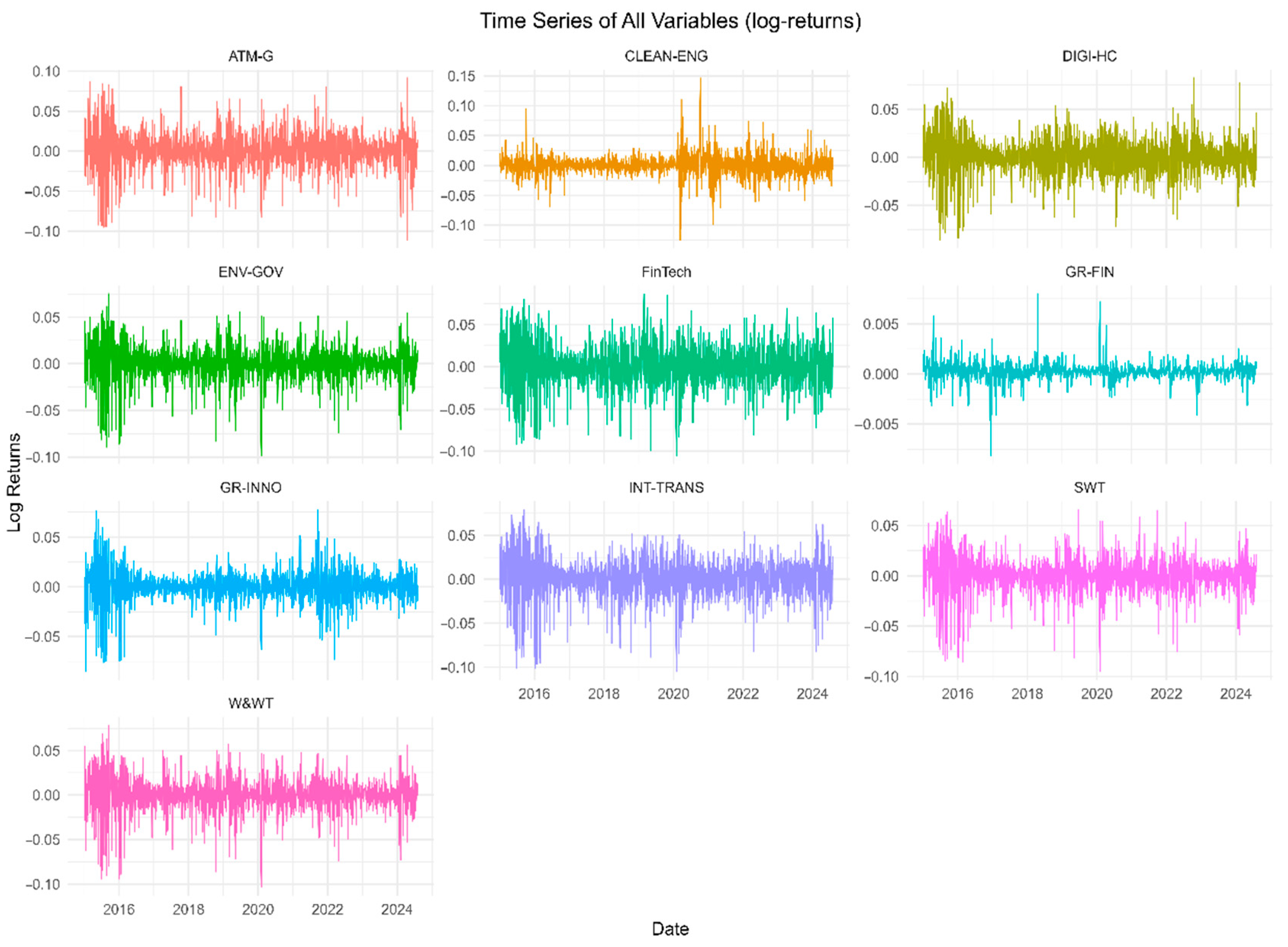
Figure 1, titled “Time Series of All Variables”, provides a visual representation of the daily return fluctuations of China’s major financial indices from January 2015 to July 2024. Table 4 summarizes the results of the stationarity tests which all confirm the stationary of time series of all variables.

4. Methodology

4.1. Quantile VAR Framework

To capture state-dependent risk spillovers, this study employs the Quantile Vector Autoregression (QVAR) framework. Unlike traditional VAR models, which focus only on average relationships, the QVAR allows coefficients to vary across different points of the return distribution. This feature is critical for analyzing dynamics in the tails of the distribution, where crises or periods of exuberance occur and where diversification benefits are most likely to break down. The QVAR therefore enables us to evaluate how shocks propagate under adverse, normal, and optimistic market states, rather than relying on mean effects that may mask extreme behavior (Ando et al., 2022; Chatziantoniou et al., 2021).

4.2. Factor-Purging Step

Before estimating the QVAR, we apply a factor-purging procedure to isolate idiosyncratic shocks. Using rolling principal component analysis, we remove common market-wide components that typically dominate financial time series. These common factors often reflect global or macroeconomic conditions and can artificially inflate spillover measures if left unaddressed. Principal Component Analysis is conducted on the matrix of standardized daily log returns (not price levels) for the ten indices. We use the correlation matrix of returns (since we standardize each series) in computing principal components. We remove the first principal component (PC1) in each window. The choice is based on the Kaiser criterion (eigenvalue > 1) and the scree plot of eigenvalues. In our data, PC1 typically has an eigenvalue far above 1 (often > 1), while PC2 is around or below 1. PC1 explains on average approximately 45% of the total variance of the 10 returns, indicating a dominant common factor (essentially a “market” factor influencing all sectors). Therefore, we opted to purge only the first factor. By focusing on idiosyncratic shocks, we sharpen inference about sector-specific channels of transmission, for example FinTech’s role in propagating liquidity shocks or environmental governance indices transmitting policy uncertainty. This adjustment improves the credibility of the connectedness measures and ensures they capture genuine intersector linkages rather than broad market co-movements (Ando et al., 2022; Chatziantoniou et al., 2021).

4.3. Forecast Error Variance Decomposition

The QVAR framework is then used to decompose the forecast error variance of each sector into portions attributable to shocks in other sectors. This decomposition shows how much of a sector’s volatility can be explained by innovations in its peers under different quantile states. For example, it allows us to quantify the share of clean energy volatility that arises from FinTech shocks during downturns. Interpreting these decompositions at the lower and upper quantiles highlights whether risk transmission strengthens in adverse states, eases in normal conditions, or becomes more balanced during optimistic periods.

4.4. Connectedness Measures

From these decompositions, we derive the connectedness indices popularized by (Diebold & Yilmaz, 2009; Diebold & Yilmaz, 2012; Diebold & Yilmaz, 2014) and adapt them to the quantile setting. The directional “TO” measure captures how much risk a sector transmits to others, while the “FROM” measure reflects how much risk it absorbs. The difference between the two gives the net connectedness, identifying systemic transmitters with positive values and receivers with negative values. The Total Connectedness Index (TCI) summarizes overall market interconnectedness as the percentage of variance explained by cross-sector shocks. Economically, a high TCI in the lower quantile indicates that shocks spread widely during crises, leaving limited room for diversification.

4.5. Inference and Robustness

We recognize that estimation uncertainty matters for interpreting connectedness measures. In this study, we present connectedness series and networks as descriptive statistics and assess robustness via rolling-window estimation and sensitivity checks over lag length, forecast horizon, and quantile selections. These checks show that our main patterns (e.g., FinTech’s transmitter role in downturns and the reduction in diversification benefits in adverse states) are qualitatively stable for reasonable modeling choices.

4.6. Comparison with Alternative Models

Finally, it is important to clarify why we employ a factor-purged QVAR rather than alternative approaches. The mean-based Diebold–Yilmaz framework (Diebold & Yilmaz, 2009, 2012, 2014) is well established but cannot capture heterogeneity across tails. Time-varying parameter VAR models allow for gradual temporal changes but still focus on average behavior rather than quantile-specific states (Antonakakis et al., 2020). Quantile-on-Quantile methods are informative but less suitable for high-dimensional systems (Chowdhury et al., 2021; Hung, 2021). Our approach combines the strengths of quantile analysis with factor-purging, enabling a tractable and interpretable framework that highlights state-contingent transmission channels. This design is particularly relevant for studying systemic spillovers, as it identifies how FinTech shocks propagate in stress periods and how policy-sensitive sectors switch roles across different market states. Quantile FEVDs allow us to trace who transmits and who absorbs shocks at specific quantiles, which is essential when risk management focuses on downside states. We employ the quantile connectedness framework of Chatziantoniou et al. (2021), we extend our analysis by incorporating a factor-purging step inspired by Ando et al. (2022). Specifically, we first extract common factors from the data using principal component analysis (PCA) on a rolling window and remove these components from the original series. This generates idiosyncratic residuals, which are then used as inputs into the quantile VAR connectedness model. In this way, our approach emphasizes the propagation of idiosyncratic shocks rather than common shocks, thereby aligning with the central insight of Ando et al. (2022) that systemic risk and spillover intensity are strongly amplified in the tails once common factors are controlled for. While we do not replicate the full quantile factor model of Ando et al. (2022), our PCA-based adaptation captures the essence of their methodology and allows us to conduct a tractable large-dimensional empirical application. we approximate their approach by purging common factors using rolling PCA, which preserves the key insight that tail spillovers are amplified once idiosyncratic shocks are isolated.
Below, Equations (2)–(14) present the methodology in one continuous sequence. Symbols: z t R n (series vector): δ ( κ ) R n is the intercept vector. F l κ   R n * n (QVAR lag matrices at quantile κ ), it is the lag-ℓ co efficient matrices, ℓ = 1, …, p and ν t κ (innovation vector at quantile), with Σ κ = V a r ν t κ , ξ h κ (VMA coefficients), e i (selection vector), and H (FEVD horizon). f i l κ R n denotes the i-th row (as a column vector) of Fℓ(κ), used in the check-loss minimization. The check loss is ρ κ u = u κ 1 { u < 0 } . In the equations, the quantile level is denoted by κ (kappa), which is identical to τ used elsewhere; thus, we take κ ≡ τ throughout, i.e., they are identical and both index the conditional quantile state (e.g., 0.10, 0.50, 0.90).
Equation (2)—QVAR ( p ) at quantile κ . Each variable depends on p lags of all variables; coefficients are specific to the evaluation quantile κ .
z t = δ κ + l = 1 p F l κ z t l + ν t κ
Equation (3)—Estimation by equation-wise quantile regression. For each i = 1 , , n , minimize the check loss to obtain { F ^ l κ } l = 1 p row by row.
m i n δ i κ , { f i l κ } t = p + 1 T ρ κ z i t δ i κ l = 1 p f i l κ z t l
Equation (4)—Quantile-specific VMA (∞) representation. Under stability at κ , shocks propagate through quantile-specific impulse responses.
z t = h = 0 Ξ h κ ν t h κ , Ξ 0 κ = I n
Equation (5)—Recursion for Ξ h κ . Compute VMA coefficients from QVAR lags via the standard companion recursion (holding κ fixed).
Ξ h κ = l = 1 m i n h , p F l κ Ξ h l κ , h = 1 , 2 ,
Equation (6)—Generalized FEVD (order-invariant). The H -step share of variable i ’s FEV due to a shock in j at quantile κ .
ϕ i j H κ = h = 0 H 1 ( e i Ξ h κ Σ κ e j ) 2 h = 0 H 1 e i Ξ h κ Σ κ Ξ h κ e i
Equation (7)—Row-normalization (shares sum to one by row). Normalize generalized shares so each row of the FEVD table is a composition of i ’s variance.
ϕ ~ i j H κ = ϕ i j H κ m = 1 n ϕ i m H κ
Equation (8)—Directional “TO” (outgoing spillovers from j ). Sum the off-diagonals in row j (impact of j on all others).
T O j H κ = i j ϕ ~ i j H κ
Equation (9)—Directional “FROM” (incoming spillovers to j ). Sum the off-diagonals in column j (impact on j from all others).
F R O M j H κ = i j ϕ ~ j i H κ
Equation (10)—Net connectedness of node j . Outgoing minus incoming.
N E T j H κ = T O j H κ F R O M j H κ
Equation (11)—Total Connectedness Index (percent scale). Off-diagonal mass of the normalized FEVD table, scaled by 100.
T C I H κ = 100 × 1 t r { Φ ~ H κ } / n , Φ ~ H κ = ϕ ~ i j H κ i , j
Equation (12)—Adjusted Total Connectedness (unit interval). A 0 , 1 index improving comparability across n .
C H κ = 1 n 1 i j ϕ ~ i j H κ
Equation (13)—Ando-style factor decomposition of innovations. Split QVAR innovations into common and idiosyncratic components at κ ; connectedness focuses on idiosyncratic shocks.
ν t κ = Λ κ g t κ + ξ t κ , Ω id κ = V a r ξ t κ
Equation (14)—Idiosyncratic GFEVD (used for spillovers). Compute FEVD with Ω id κ and shocks ξ t κ (same formula as (Equation (6), different inputs).
ϕ i j ; id H κ = h = 0 H 1 ( e i Ξ h κ Ω id κ e j ) 2 h = 0 H 1 e i Ξ h κ Ω id κ Ξ h κ e i
(i) κ is held fixed throughout each evaluation (QVAR, VMA, FEVD), (ii) the generalized scheme avoids Cholesky ordering and is row-normalized, (iii) when factor-purging is used, all connectedness metrics are built from Equation (14). Typical choices: p = 1 by BIC at κ   τ = 0.10 ,   0.50 ,   0.90 ; H { 10 } ; rolling window W 250 for time variation.

5. Results and Discussion

5.1. Dynamic Total Connectedness (TCI) Across Quantiles

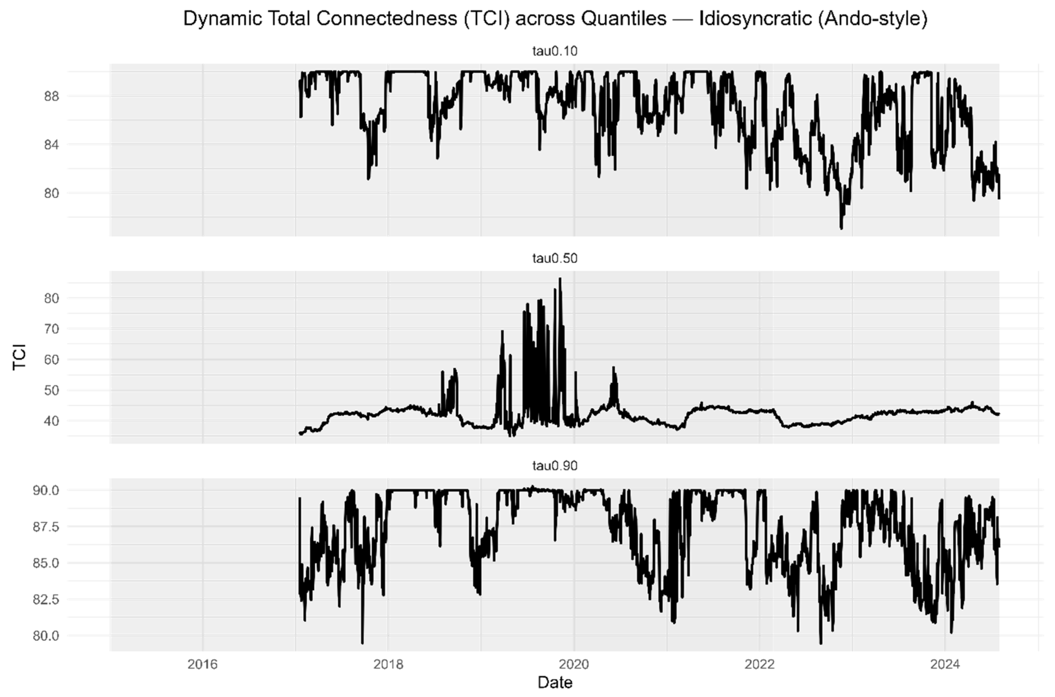
Figure 2 plots the dynamic Total Connectedness Index (TCI) obtained from the QVAR–GFEVD at τ ∈ {0.10, 0.50, 0.90}. The first result concerns the overall level of connectedness across sectors. The Total Connectedness Index (TCI) is consistently higher in the lower quantile (τ = 0.10) compared with the median (τ = 0.50) and the upper quantile (τ = 0.90). This pattern indicates that shocks spread more intensively during adverse market conditions, confirming the presence of tail amplification. In practical terms, diversification benefits diminish precisely when investors need them most, as downside states tighten risk linkages across FinTech and sustainability sectors. Episodes such as the COVID-19 outbreak and subsequent policy adjustments are accompanied by pronounced surges in TCI, showing that systemic shocks compress risk buffers across the entire system.

5.2. Full-Sample Spillover Networks at τ = 0.10, 0.50, and 0.90

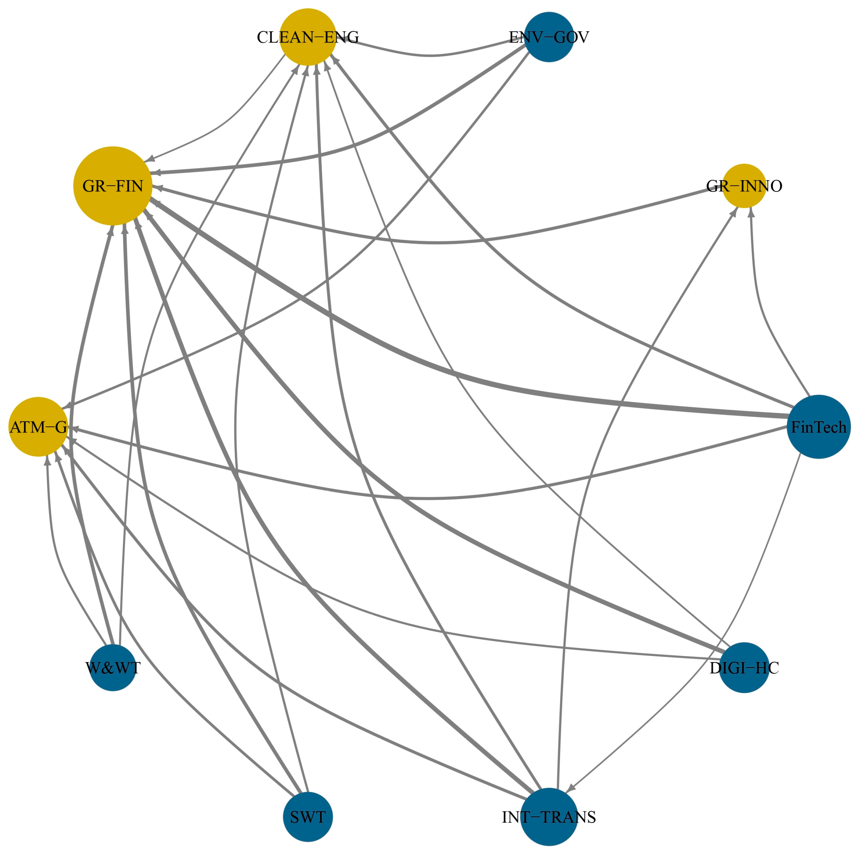
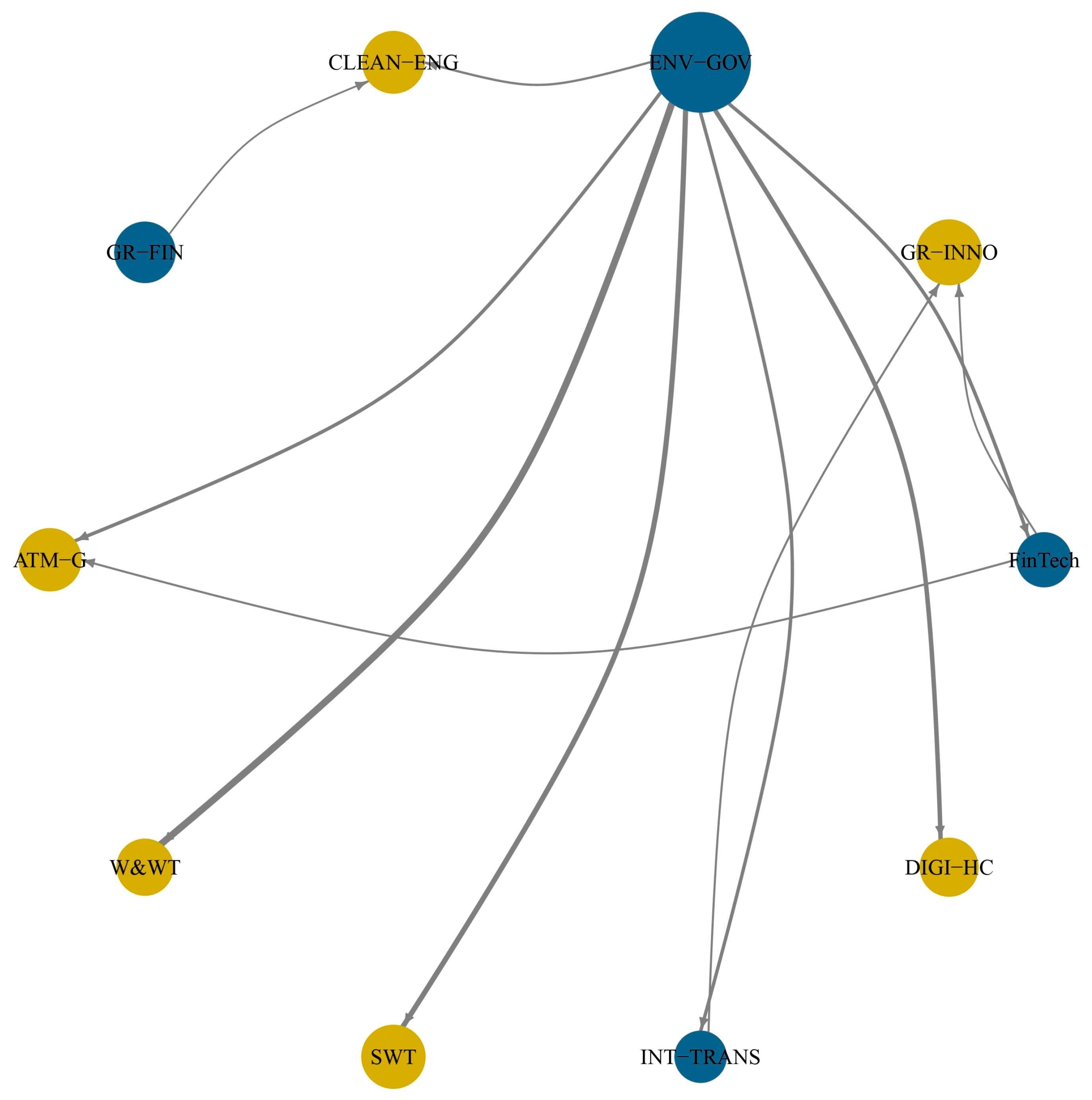
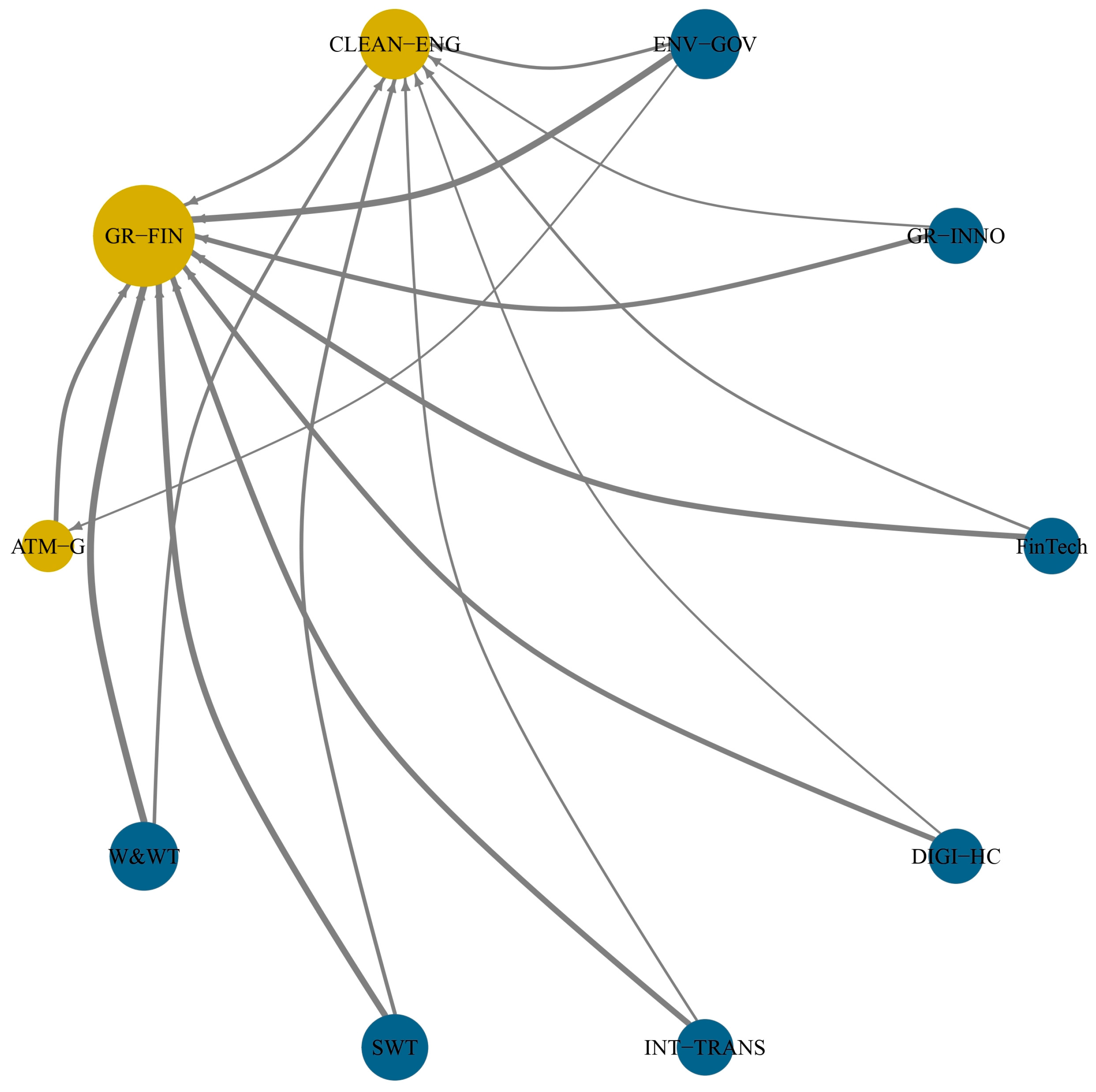
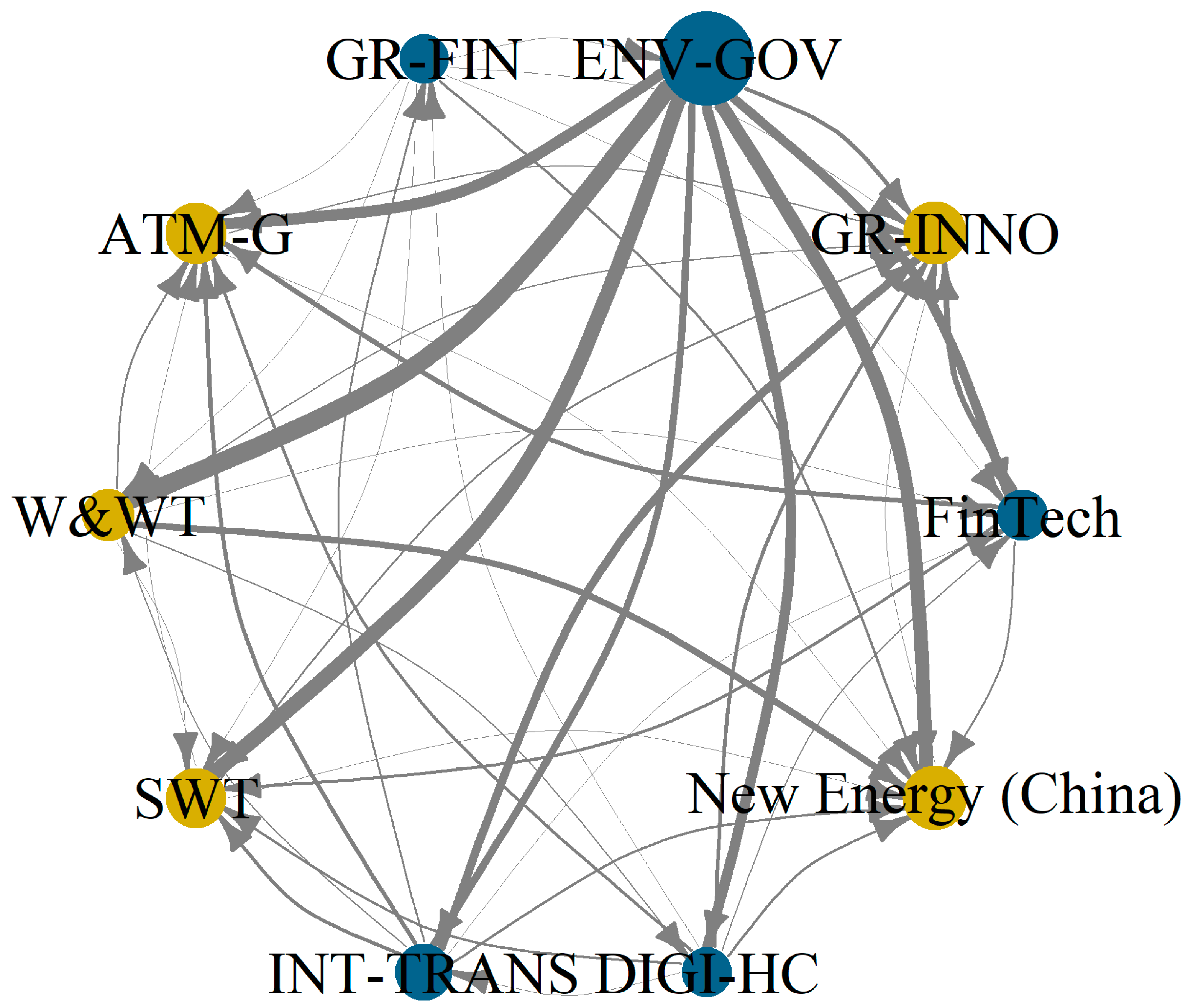
Figure 3, Figure 4 and Figure 5 display the directed, weighted spillover networks (full sample) at the lower, median, and upper quantiles. Spillover networks at different quantiles provide further insight into the structure of risk transmission.
At τ = 0.10 (adverse state), FinTech emerges as a central transmitter, sending significant spillovers to clean energy and green innovations. This supports the funding channel (H1), where liquidity and credit shocks originating in FinTech cascade into capital-intensive sustainability sectors.
Policy-related indices, such as environmental and atmospheric governance, also act as transmitters under stress, consistent with the policy asymmetry channel (H2).
Clean energy and green innovations tilt toward receiver roles, absorbing shocks rather than generating them, highlighting their vulnerability to financing conditions.
At τ = 0.50 (median state), spillovers are more balanced, with fewer dominant transmitters. Policy indices absorb more than they transmit, reflecting stabilization during normal conditions.
At τ = 0.90 (optimistic state), the network becomes sparser and two-way interactions dominate. FinTech’s transmitter role weakens, while digital verticals such as healthcare and intelligent transport take on more active positions. This supports H3, where technology-driven sectors partially transmit shocks in positive states, driven by demand rebounds and platform growth.

5.3. Quantile Asymmetry (Upper−Lower TCI Proxy)

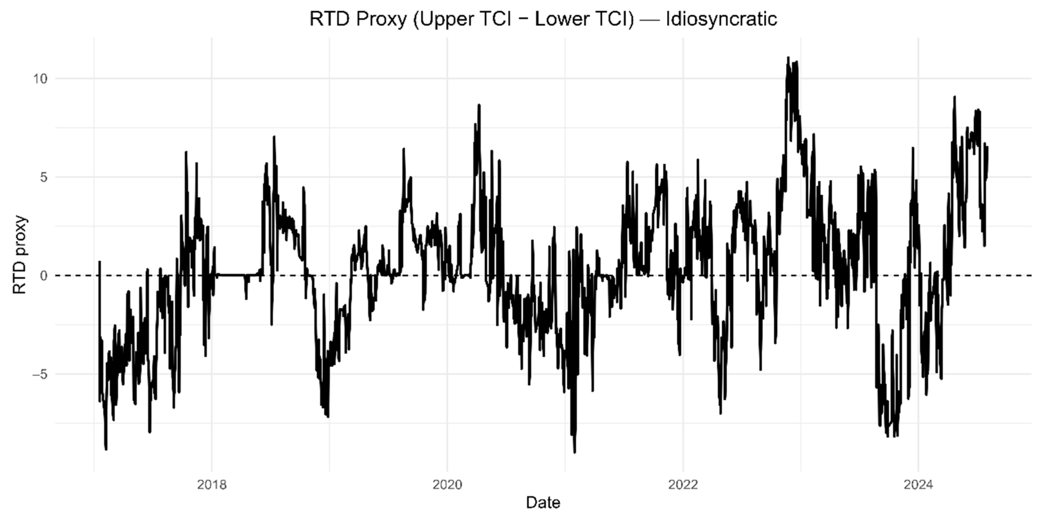
Figure 6 charts an asymmetry proxy defined as TCI (τ = 0.90) − TCI (τ = 0.10). Comparing TCI between upper and lower quantiles shows that adverse states generally dominate optimistic ones. The difference measure (TCI at τ = 0.90 minus TCI at τ = 0.10) is negative during systemic stress periods, confirming that downside shocks bind sectors more tightly. Occasional positive spikes suggest that optimistic extremes can also generate strong spillovers, but these episodes are less frequent and less persistent. The overall evidence confirms H5, that diversification benefits are compressed in both tails but especially in the left tail.

5.4. Directional Roles and Channels

Synthesizing the results across metrics and hypotheses yields four main observations:
Funding/Liquidity (H1): FinTech and green finance consistently act as transmitters in downturns. Their role as providers of credit and liquidity means that stress in these sectors propagates to clean energy and green innovations.
Policy/Regulation (H2): Environmental and atmospheric governance indices are state-dependent. They transmit shocks during stress but absorb shocks during calmer or optimistic periods. This asymmetry reflects the regulatory environment, where policy tightening amplifies risks but policy relaxation provides relief.
Technology–Real Economy Coupling (H3): Digital healthcare and intelligent transportation absorb more spillovers in downturns but switch to mild transmitters in optimistic conditions. This highlights the pro-cyclical nature of platform-based sectors.
Environmental Services (H4): Water and waste utilities remain net receivers, especially in the lower quantile, underscoring their limited flexibility under financial or policy stress.

5.5. Economic and Policy Implications

The results carry important lessons for both investors and policymakers. For portfolio managers, the evidence demonstrates that diversification across FinTech and sustainability sectors is fragile under stress, and risk budgeting must explicitly account for quantile-specific dynamics. In practical terms, this means investors should monitor tail risk indicators. For instance, if they track a rising TCI at the 10th percentile (perhaps using techniques from this paper), that could warn that their cross-sector diversification is breaking down. Portfolio managers should consider hedging strategies designed for adverse states: e.g., buying protective puts on FinTech index or related ETFs when downside connectedness metrics rise, or reducing exposure to multiple sustainability sectors that tend to crash together. Traditional mean-variance optimization won’t capture these nonlinear correlations; a quantile-based approach (minimizing Conditional Value-at-Risk, for example) might be more appropriate. Our findings specifically suggest that FinTech can be a “risk conduit” so hedging or under-weighting FinTech during times of financial tightening could lower overall portfolio risk. Also, since policy-heavy sectors get hit in crises, investors might demand higher risk premiums for those sectors knowing their asymmetric risk profile. Hedging strategies need to be designed for adverse states, where FinTech shocks in particular compromise capital-intensive sectors.
For regulators, the asymmetric role of policy-intensive nodes calls for careful monitoring of regulatory spillovers during uncertainty, as these can accelerate systemic risk transmission. Stress tests that focus only on average conditions risk underestimating vulnerabilities; instead, regulators should simulate downside-tail scenarios where systemic linkages are strongest. Regulators (such as the People’s Bank of China or the China Banking and Insurance Regulatory Commission) should incorporate downside-tail scenarios in their macroprudential stress testing. For example, they could simulate a scenario where FinTech lending drops by, say, 30% (a severe contraction reflecting a FinTech credit crunch), and examine the impact on clean energy firms’ solvency or on green bond spreads effectively a multi-sector stress scenario. Our results suggest that scenario would show significant knock-on effects, justifying measures to counteract it (like emergency liquidity to sustainable projects or encouraging banks to step in if FinTech pulls back). Secondly, the findings underscore that policy uncertainty can amplify systemic risk in bad times. Thus, regulators might strive for stable and clear communication of environmental policies especially during market stress, to avoid adding fuel to the fire. If possible, major new carbon regulations or green financing rules might be better introduced during stable times, whereas in a crisis, providing reassurance (or even relaxing some requirements temporarily) could avoid exacerbating the financial turmoil in sustainability sectors. Lastly, given FinTech’s systemic role, regulators might consider macroprudential tools targeting FinTech for instance, requiring FinTech platforms to maintain certain loss-absorbing buffers or subjecting them to stress tests alongside banks. This would be analogous to how systemically important banks are regulated, extending some of that mindset to large FinTech firms.
In terms of broader policy, our results align with the agenda of “greening” the financial system but add nuance: a resilient green financial system may need buffers for when multiple green sectors get hit simultaneously (like renewable energy, water, waste all suffering together in a downturn). The network perspective can inform cross-sector policy coordination: e.g., if the Ministry of Finance is designing a green stimulus, they might target it to sectors that are receivers (like water/waste utilities) during downturns to shore them up and prevent cascade, or ensure FinTech credit keeps flowing to clean energy projects in a slump perhaps through guarantees.

6. Conclusions

This paper provides novel evidence on tail-dependent spillovers between Chinese FinTech and sustainability-linked sectors using a factor-purged quantile connectedness framework. Three findings stand out. First, FinTech consistently emerges as a net transmitter in adverse states, underscoring its role in propagating liquidity and credit shocks. When markets turn down, shocks originating in China’s FinTech sector (e.g., tighter online credit, fintech market corrections) spread forcefully to other sectors like clean energy and green finance, amplifying system-wide risk. Second, diversification benefits compress when risks are highest, as stronger connectedness erodes cross-sector hedging opportunities. Investors holding a portfolio of FinTech, renewable energy, and environmental assets will find limited refuge in a crisis as contagion ties their fates together. Third, policy-intensive nodes switch roles asymmetrically across quantiles, reflecting regulatory spillovers that intensify during uncertainty but attenuate in stable conditions. Sectors tied to environmental regulation (environmental governance, atmospheric governance) transmit shocks under stress, reflecting how policy uncertainty or stringent rules bite in bad times, but they become shock absorbers or neutral in stable/optimistic periods. This asymmetry highlights that regulatory impact on financial markets is highly state-dependent.
These results have important implications. For portfolio managers, they caution that diversification strategies relying on sustainable sectors may fail precisely during downturns, requiring quantile-aware risk budgeting and dynamic hedging. In practice, this means incorporating tail-risk measures (like our quantile connectedness metrics or scenario analysis) into portfolio construction. Portfolio hedges should be designed with stress scenarios in mind, for example hedging FinTech exposure or adding uncorrelated assets when our indicators show rising lower-tail connectedness. For regulators, the asymmetric roles of policy sectors call for stress testing at the tails, with a focus on FinTech-linked liquidity channels and climate policy announcement windows. Regulators should simulate worst-case tail scenarios (e.g., a FinTech credit crunch coinciding with a climate policy shock) to see how financial institutions and markets cope. Such quantile-focused stress tests could be integrated into China’s regulatory toolkit, complementing traditional tests. Additionally, our findings suggest that regulators monitor FinTech as a potential amplifier of systemic risk and ensure liquidity support or safeguards for sustainable sectors during extreme events. They also underscore the need for clear policy communication: abrupt environmental policy moves in an already fragile market can accelerate a downturn, so a calibrated approach to policy implementation is advised during stressed conditions.
Finally, while quantile connectedness measures forecast-variance contributions rather than structural causality, our approach enhances transparency and robustness through factor-purging and extensive sensitivity checks. Future research could extend this framework to cross-country comparisons, integrate event-study identification around policy shocks, or apply quantile SVAR methods to strengthen causal interpretation.
In conclusion, the FinTech–sustainability nexus in China exhibits complex, state-dependent risk transmission. By focusing on tail events, we reveal that the very moments when these sectors are needed for stability (e.g., as diversifiers or shock absorbers) are when they instead synchronize and amplify risk. This insight is crucial for designing resilient portfolios and effective regulatory policies in an era where both digital finance and sustainable investments are increasingly central. We hope that our quantile-based network approach provides a useful template for analyzing such systemic interactions under extreme conditions.

Supplementary Materials

The following supporting information can be downloaded at: https://www.mdpi.com/article/10.3390/ijfs13040218/s1, supplementary materials: Theoretical Framework Diagram.

Author Contributions

Conceptualization, K.P. and M.M. (Muhammad Munir); methodology, K.P., M.M. (Muhammad Munir) and M.M. (Mariem Mejri); software, M.M. (Muhammad Munir); validation, K.P., M.M. (Muhammad Munir), J.R. and M.M. (Mariem Mejri); formal analysis, M.M. (Muhammad Munir); investigation, M.M. (Muhammad Munir); resources, K.P., M.M. (Muhammad Munir), J.R. and M.M. (Mariem Mejri); data curation, M.M. (Muhammad Munir); writing—original draft preparation, M.M. (Muhammad Munir); writing—review & editing, K.P., M.M. (Muhammad Munir), J.R. and M.M. (Mariem Mejri); visualization, K.P., J.R. and M.M. (Mariem Mejri); supervision, K.P. and J.R.; project administration, K.P. and J.R.; funding acquisition, K.P. and M.M. (Mariem Mejri). All authors have read and agreed to the published version of the manuscript.

Funding

The authors acknowledge the funding support from Shenzhen Key Research Base of Humanities and Social Sciences (KP191003), University-Industry Collaborative Education Program (202002311004), Shenzhen Science and Technology Program (No. SYSPG 20241211173609007) and the Social Science Foundation of Harbin Institute of Technology, Shenzhen, China. The authors also acknowledge the financial support and facilitation from University of Sahiwal, Sahiwal, Punjab, Pakistan to conduct this research. This research is supported by the Shenzhen Science and Technology Program (Grants No. RKX20231110090859012), Shenzhen Humanities and Social Sciences Key Research Bases (Grants No. KP191001), Shenzhen Nanshan District Education Science Planning Project “Research on the Application of Intelligent Assisted Teaching in Primary School English Courses”; Harbin Institute of Technology (Shenzhen) joint basic education training project “Application project of intelligent assisted teaching system for middle school biology courses based on multimodal large language model”.

Institutional Review Board Statement

Not applicable.

Informed Consent Statement

Not applicable.

Data Availability Statement

The data used in this study were obtained from the wind database, which provides publicly accessible data. All datasets used are available to registered users through the wind data platform. Interested researchers can access the data by creating an account at https://www.wind.com.cn (accessed on 4 August 2024). Further details can be provided upon request from the corresponding authors.

Acknowledgments

The authors acknowledge the support from Social Science Foundation of Harbin Institute of Technology, Shenzhen, China. The authors would like to express their sincere gratitude to Prince Sultan University, Riyadh, Saudi Arabia, for providing technical knowledge transfer and valuable support throughout this research. The authors also extend their appreciation to the University of Sahiwal, Sahiwal, Punjab, Pakistan, for its support and facilitation in carrying out this study.

Conflicts of Interest

The authors declare no conflicts of interest.

Appendix A. Robustness Analysis—Wind New Energy Index (Only China Specific Clean Energy Proxy)

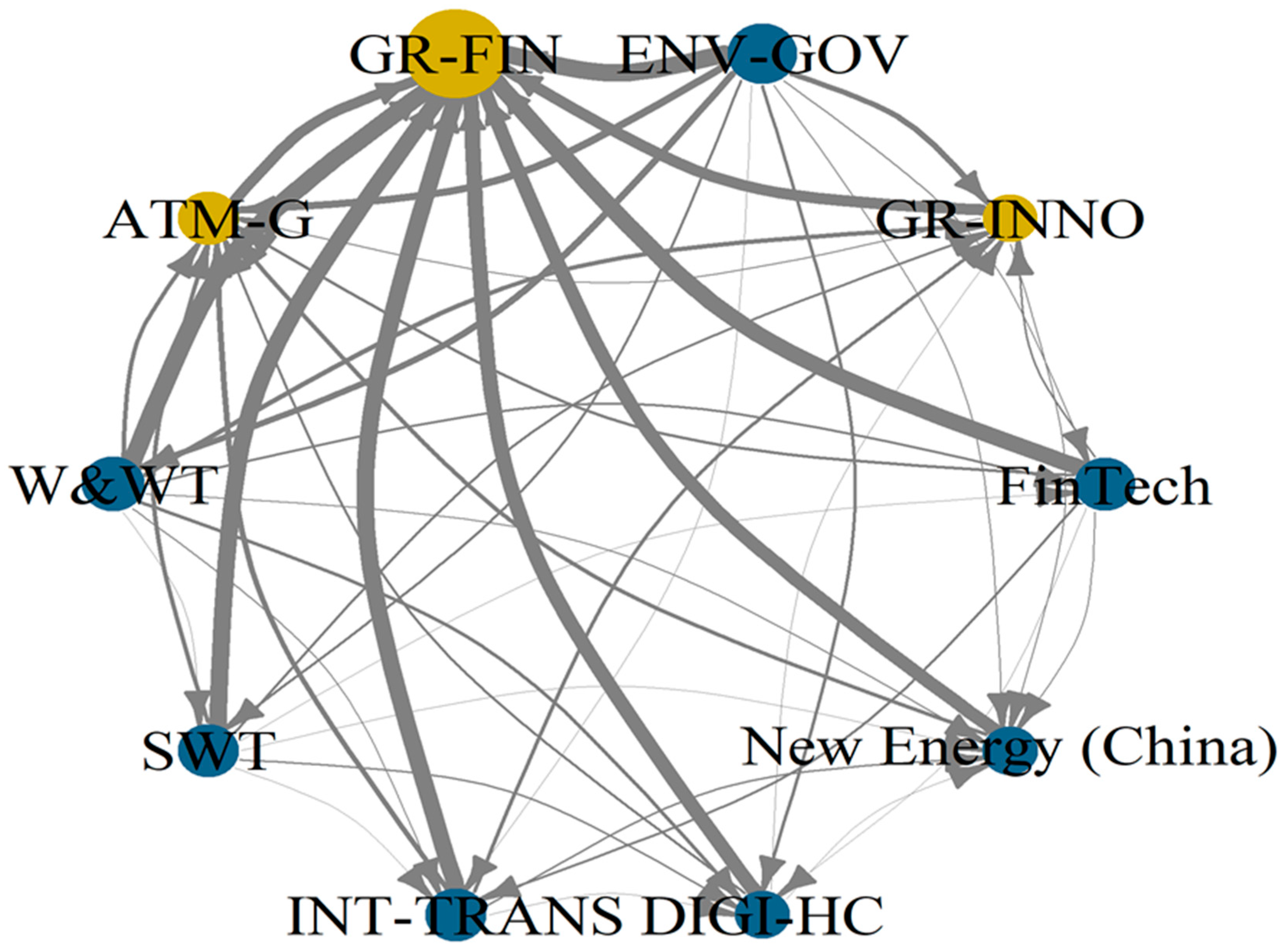
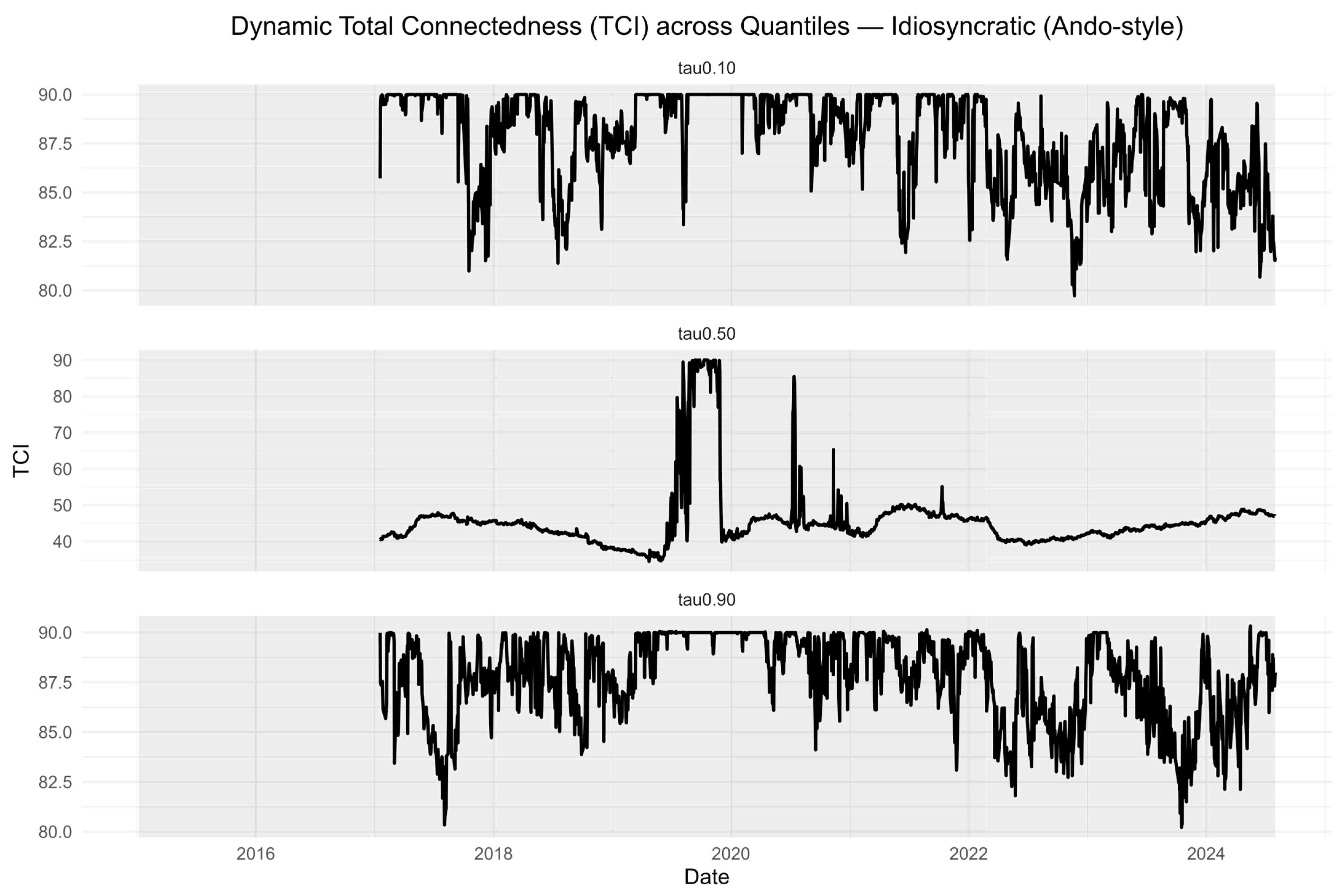
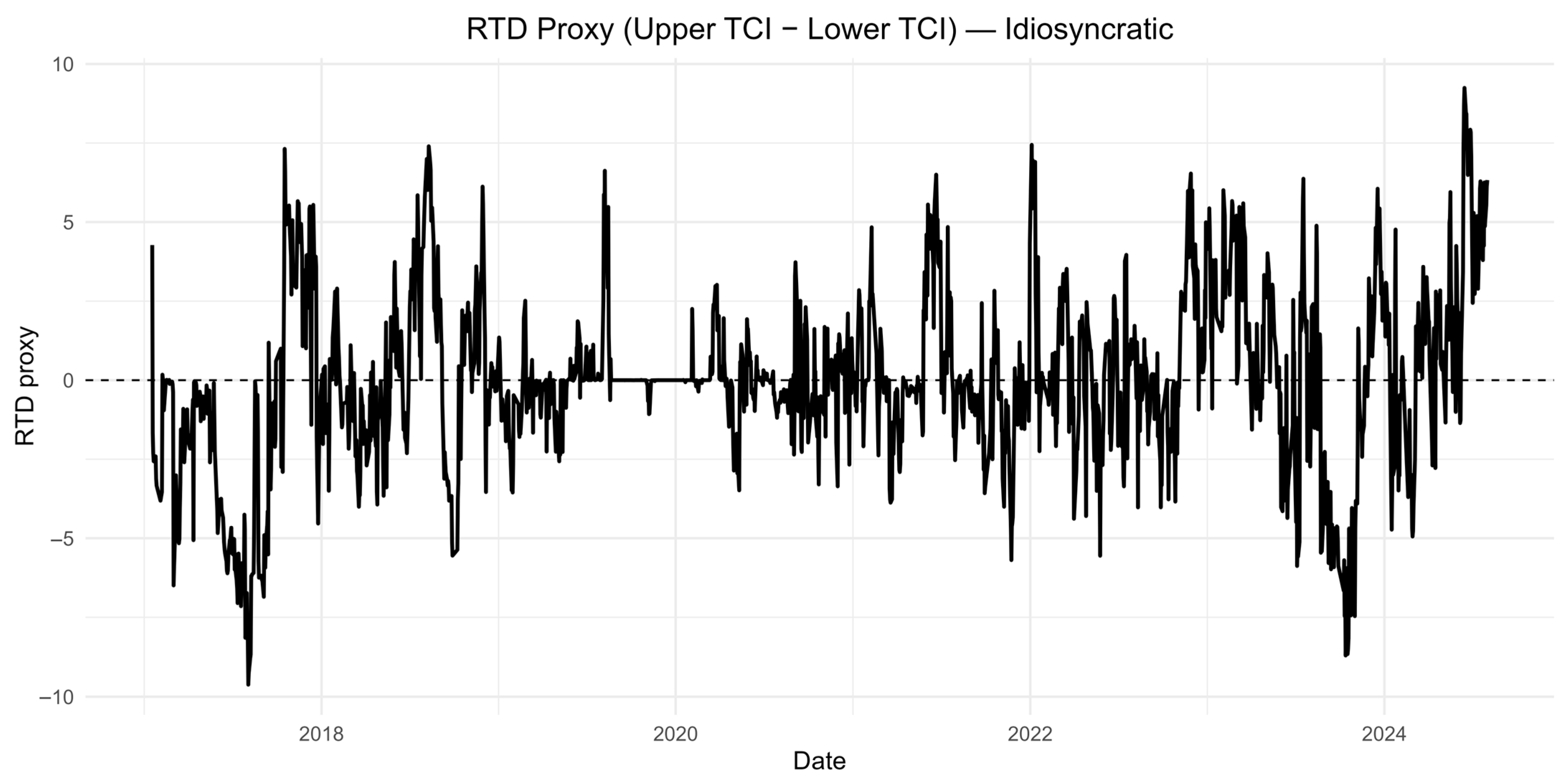
To ensure our findings are not driven by the choice of clean energy proxy, we conducted a robustness check by replacing the original S & P Clean Energy Index with the China-specific Wind New Energy Index, which tracks China’s renewable energy sector. The connectedness analysis under this alternative specification remains qualitatively consistent with our main results. In particular, FinTech continues to act as a net transmitter of tail risk in the lower-tail state (τ = 0.10, 0.50, 0.90), while the clean energy sector (proxied by the Wind New Energy Index) remains a net receiver at (τ = 0.50), absorbing more shocks than it transmits. The median (τ = 0.50) and upper-tail (τ = 0.90) network structures under the Wind New Energy Index are similarly in line with those reported in the main analysis, showing balanced spillovers at the median state and a weaker FinTech influence in optimistic conditions. This robustness exercise confirms that our key conclusions hold true even when using a China-specific clean energy benchmark. (See Appendix A, Figure A1, Figure A2, Figure A3, Figure A4 and Figure A5 and Table A1, Table A2 and Table A3 and the Table A4, Table A5 and Table A6 provides connectedness tables of original study (global clean energy proxy) for comparison), thereby reinforcing the reliability of the results.
Figure A1. Network_Full_Sample_tau τ = 0.10 (Lower-tail network) with China specific Clean Energy Proxy. (Wind New Energy Index).
Ijfs 13 00218 g0a1
Figure A2. Network_Full_Sample_tau τ = 0.50 (Median network) with China specific Clean Energy Proxy. (Wind New Energy Index).
Ijfs 13 00218 g0a2
Figure A3. Network_Full_Sample_tau τ = 0.90_ (Upper-tail network) with China specific Clean Energy Proxy. (Wind New Energy Index).
Ijfs 13 00218 g0a3
Figure A4. Dynamic Total Connectedness across Quantiles with China specific Clean Energy Proxy. (Wind New Energy Index).
Ijfs 13 00218 g0a4
Figure A5. RTD Proxy (Upper TCI − Lower TCI) with China specific Clean Energy Proxy. (Wind New Energy Index).
Ijfs 13 00218 g0a5
Table A1. Connectedness Table-Full Sample at (τ = 0.10) with China specific Clean Energy Proxy. (Wind New Energy Index).
SectorFinTechGR-INNOENV-GOVGR-FINATM-GW&WTSWTINT-TRANSDIGI-HCNew Energy (China)FROM
FinTech13.419.189.018.648.89.279.5211.710.599.8786.59
GR-INNO10.2412.039.698.699.249.6910.269.879.9910.387.97
ENV-GOV9.899.4611.558.619.8511.0410.819.649.69.5388.45
GR-FIN10.359.619.6811.159.339.6810.0210.0710.29.9188.85
ATM-G10.089.410.398.7512.019.869.999.949.729.8587.99
W&WT9.939.511.58.549.512.2410.259.679.539.3387.76
SWT10.119.6410.688.789.2610.0611.989.779.99.8288.02
INT-TRANS12.229.018.858.698.849.159.2813.6610.549.7786.34
DIGI-HC11.019.529.38.778.929.379.9310.5912.3310.2687.67
New Energy (China)10.52109.358.699.299.339.9410.1910.3912.2987.71
TO94.3485.3488.4578.1683.0487.469091.4590.4888.63877.35
Inc.Own107.7597.3710089.3195.0599.7101.98105.11102.81100.92cTCI/TCI
NET7.75−2.630−10.69−4.95−0.31.985.112.810.9297.48/87.73
NPT9240147864
Table A2. Connectedness Table-Full Sample at (τ = 0.50) with China specific Clean Energy Proxy. (Wind New Energy Index).
SectorFinTechGR-INNOENV-GOVGR-FINATM-GW&WTSWTINT-TRANSDIGI-HCNew Energy (China)FROM
FinTech43.523.9213.331.575.176.926.6813.034.351.556.48
GR-INNO6.2266.663.051.342.821.712.478.434.492.8133.34
ENV-GOV9.741.4630.391.315.5818.589.3997.916.6369.61
GR-FIN1.440.931.387.151.711.021.171.862.351.0712.85
ATM-G7.162.369.861.7557.222.041.566.367.813.8842.78
W&WT6.541.225.561.061.3142.442.126.346.76.7157.56
SWT7.971.7915.161.171.372.452.518.894.444.3147.49
INT-TRANS12.885.1111.821.024.665.767.3446.763.411.2453.24
DIGI-HC3.873.0611.752.196.537.233.493.3756.691.8143.31
New Energy (China)2.392.5711.9324.039.224.382.212.8458.4241.58
TO58.2222.4103.7513.4233.1954.938.6159.4944.329.96458.24
Inc.Own101.7489.06134.15100.5890.497.3491.11106.25100.9988.38cTCI/TCI
NET1.74−10.9434.150.58−9.6−2.66−8.896.250.99−11.6250.92/45.82
NPT4087263771
Table A3. Connectedness Table-Full Sample at (τ = 0.90) with China specific Clean Energy Proxy. (Wind New Energy Index).
SectorFinTechGR-INNOENV-GOVGR-FINATM-GW&WTSWTINT-TRANSDIGI-HCNew Energy (China)FROM
FinTech12.249.599.758.079.249.789.7111.1610.489.9787.76
GR-INNO9.8411.9210.388.289.5110.2410.159.789.7910.1288.08
ENV-GOV9.619.6412.057.969.9811.2810.959.549.529.4787.95
GR-FIN10.089.710.1510.99.59.9710.0510.019.869.7889.1
ATM-G9.659.6610.98.2312.2310.2610.049.79.549.7987.77
W&WT9.499.6212.087.939.7312.6810.39.529.399.2687.32
SWT9.669.8211.288.129.5110.3312.289.529.79.7987.72
INT-TRANS11.59.329.588.099.069.679.5512.9310.419.9187.07
DIGI-HC10.69.699.888.179.219.819.9610.4912.0710.1287.93
New Energy (China)10.1210.279.628.169.289.469.910.1410.1212.9287.08
TO90.5587.393.6273.0285.0290.890.6189.8688.8188.2877.79
Inc.Own102.7999.22105.6783.9197.25103.48102.89102.79100.88101.12cTCI/TCI
NET2.79−0.785.67−16.09−2.753.482.892.790.881.1297.53/87.78
NPT6390187542
Table A4. Connectedness Table-Full Sample at (τ = 0.10) with S&P Global Clean Energy Index.
SectorFinTechGR-INNOENV-GOVCLEAN-ENGGR-FINATM-GW&WTSWTINT-TRANSDIGI-HCFROM
FinTech13.449.439.069.468.588.719.369.4911.7910.6886.56
GR-INNO10.2112.759.789.58.639.079.8310.279.9210.0487.25
ENV-GOV9.219.3613.018.688.439.9111.9411.369.099.0186.99
CLEAN-ENG10.599.879.5512.268.619.129.629.910.2910.1987.74
GR-FIN10.479.749.719.1811.589.199.719.9110.2510.2688.42
ATM-G9.779.4810.799.28.7212.8310.029.939.799.4787.17
W&WT9.739.5611.98.918.469.2512.9810.219.569.4587.02
SWT9.919.8811.149.18.658.9610.0612.759.659.987.25
INT-TRANS12.359.138.859.278.678.729.189.213.9610.6786.04
DIGI-HC11.129.619.149.568.668.719.279.7910.7613.3886.62
TO93.3586.0589.9282.8677.4181.648990.0591.189.68871.05
Inc.Own106.898.8102.9295.1188.9994.47101.98102.79105.07103.06cTCI/TCI
NET6.8−1.22.92−4.89−11.01−5.531.982.795.073.0696.78/87.11
NPT9352015686
Table A5. Connectedness Table-Full Sample at (τ = 0.50) with S&P Global Clean Energy Index.
SectorFinTechGR-INNOENV-GOVCLEAN-ENGGR-FINATM-GW&WTSWTINT-TRANSDIGI-HCFROM
FinTech41.943.3116.381.061.645.657.916.711.943.4858.06
GR-INNO5.4869.573.561.112.533.011.982.796.753.2330.43
ENV-GOV12.391.6531.742.351.875.0117.978.9410.028.0668.26
CLEAN-ENG1.111.24.9779.032.991.973.352.571.31.5120.97
GR-FIN1.120.911.580.9689.161.811.041.131.021.2810.84
ATM-G8.042.4991.322.4860.041.581.356.217.4939.96
W&WT8.11.2525.742.111.130.9945.861.327.126.3954.14
SWT8.432.3914.862.061.631.521.7355.498.193.744.51
INT-TRANS12.614.3913.870.821.514.826.76.9145.622.7554.38
DIGI-HC3.752.4913.141.022.476.627.633.482.8956.5243.48
TO61.0320.08103.112.8218.2331.449.8935.1955.4437.88425.05
Inc.Own102.9689.64134.8491.85107.3991.4495.7590.67101.0694.4cTCI/TCI
NET2.96−10.3634.84−8.157.39−8.56−4.25−9.331.06−5.647.23/42.50
NPT7180935264
Table A6. Connectedness Table-Full Sample at (τ = 0.90) with S&P Global Clean Energy Index.
SectorFinTechGR-INNOENV-GOVCLEAN-ENGGR-FINATM-GW&WTSWTINT-TRANSDIGI-HCFROM
FinTech13.089.729.349.38.019.259.649.6611.4510.5486.92
GR-INNO9.6412.5510.199.368.229.7810.3110.419.729.8287.45
ENV-GOV8.989.7712.728.877.9610.2911.8711.229.039.2887.28
CLEAN-ENG10.2210.129.9411.58.019.7610.0810.2510.0310.0988.5
GR-FIN9.889.8410.079.1511.349.7110.0910.0810.019.8388.66
ATM-G9.399.9210.979.318.212.9110.3810.079.529.3487.09
W&WT9.159.8512.228.947.869.8713.310.339.239.2486.7
SWT9.3110.1511.4398.079.610.39139.389.6687
INT-TRANS11.339.649.499.178.149.349.799.8212.8610.4287.14
DIGI-HC10.629.99.579.368.19.299.7210.0410.4412.9587.05
TO88.5288.9193.2382.4672.5886.9192.2691.8888.8188.23873.8
Inc.Own101.6101.46105.9593.9683.9299.82105.56104.88101.67101.18cTCI/TCI
NET1.61.465.95−6.04−16.08−0.185.564.881.671.1897.09/87.38
NPT4591028763

References

  1. Aharon, D. Y., Demir, E., & Umar, Z. (2025). On the connectedness between climate policy uncertainty, green bonds, and equity. Modern Finance, 3(1), 25–37. [Google Scholar] [CrossRef]
  2. Ando, T., Greenwood-Nimmo, M., & Shin, Y. (2022). Quantile connectedness: Modeling tail behavior in the topology of financial networks. Management Science, 68(4), 2401–2431. [Google Scholar] [CrossRef]
  3. Anscombe, F. J., & Glynn, W. J. (1983). Distribution of the kurtosis statistic-B2 for normal samples. Biometrika, 70(1), 227–234. [Google Scholar] [CrossRef]
  4. Antonakakis, N., Chatziantoniou, I., & Gabauer, D. (2020). Refined measures of dynamic connectedness based on time-varying parameter vector autoregressions. Journal of Risk and Financial Management, 13(4), 84. [Google Scholar] [CrossRef]
  5. Baker, M., Bergstresser, D., Serafeim, G., & Wurgler, J. (2022). The pricing and ownership of US green bonds. Annual Review of Financial Economics, 14(1), 415–437. [Google Scholar] [CrossRef]
  6. Bestsennyy, O., Gilbert, G., Harris, A., & Rost, J. (2021). Telehealth: A quarter-trillion-dollar post-COVID-19 reality. McKinsey & Company. Available online: https://www.mckinsey.com/industries/healthcare-systems-and-services/our-insights/telehealth-a-quarter-trillion-dollar-post-covid-19-reality (accessed on 5 September 2025).
  7. Bolton, P., & Kacperczyk, M. (2021). Do investors care about carbon risk? Journal of Financial Economics, 142(2), 517–549. [Google Scholar] [CrossRef]
  8. Chatziantoniou, I., Gabauer, D., & Stenfors, A. (2021). Interest rate swaps and the transmission mechanism of monetary policy: A quantile connectedness approach. Economics Letters, 204, 109891. [Google Scholar] [CrossRef]
  9. Chen, R., Chen, H., Jin, C., Wei, B., & Yu, L. (2020). Linkages and spillovers between internet finance and traditional finance: Evidence from China. Emerging Markets Finance and Trade, 56(6), 1196–1210. [Google Scholar] [CrossRef]
  10. Choi, S.-Y. (2022). Dynamic volatility spillovers between industries in the US stock market: Evidence from the COVID-19 pandemic and Black Monday. The North American Journal of Economics and Finance, 59, 101614. [Google Scholar] [CrossRef]
  11. Chowdhury, M. A. F., Meo, M. S., & Aloui, C. (2021). How world uncertainties and global pandemics destabilized food, energy and stock markets? Fresh evidence from quantile-on-quantile regressions. International Review of Financial Analysis, 76, 101759. [Google Scholar] [CrossRef]
  12. Claessens, S., Frost, J., Turner, G., & Zhu, F. (2018). Fintech credit markets around the world: Size, drivers and policy issues. BIS Quarterly Review September 2018. Available online: https://ssrn.com/abstract=3288096 (accessed on 5 September 2025).
  13. D’Agostino, R. B. (1970). Transformation to normality of the null distribution of g 1. Biometrika, 57(3), 679–681. [Google Scholar] [CrossRef]
  14. Deng, L., Lv, Y., Liu, Y., & Zhao, Y. (2021). Impact of fintech on bank risk-taking: Evidence from China. Risks, 9(5), 99. [Google Scholar] [CrossRef]
  15. Diebold, F. X., & Yilmaz, K. (2009). Equity market spillovers in the Americas. Economia Chilena, 12(2), 55–65. [Google Scholar]
  16. Diebold, F. X., & Yilmaz, K. (2012). Better to give than to receive: Predictive directional measurement of volatility spillovers. International Journal of Forecasting, 28(1), 57–66. [Google Scholar] [CrossRef]
  17. Diebold, F. X., & Yilmaz, K. (2014). On the network topology of variance decompositions: Measuring the connectedness of financial firms. Journal of Econometrics, 182(1), 119–134. [Google Scholar] [CrossRef]
  18. Egli, F., Steffen, B., & Schmidt, T. (2018). A dynamic analysis of financing conditions for renewable energy technologies. Nature Energy, 3(12), 1084–1092. [Google Scholar] [CrossRef]
  19. Elliott, G., Rothenberg, T. J., & Stock, J. H. (1996). Efficient tests for an autoregressive unit root. Econometrica, 64(4), 813–836. [Google Scholar] [CrossRef]
  20. Fang, Y., Wang, Q., Wang, F., & Zhao, Y. (2023). Bank fintech, liquidity creation, and risk-taking: Evidence from China. Economic Modelling, 127, 106445. [Google Scholar] [CrossRef]
  21. Flammer, C. (2021). Corporate green bonds. Journal of Financial Economics, 142(2), 499–516. [Google Scholar] [CrossRef]
  22. Giglio, S., Kelly, B., & Pruitt, S. (2016). Systemic risk and the macroeconomy: An empirical evaluation. Journal of Financial Economics, 119(3), 457–471. [Google Scholar] [CrossRef]
  23. Hung, N. T. (2021). Bitcoin and CEE stock markets: Fresh evidence from using the DECO-GARCH model and quantile on quantile regression. European Journal of Management and Business Economics, 30(2), 261–280. [Google Scholar] [CrossRef]
  24. Jarque, C. M., & Bera, A. K. (1980). Efficient tests for normality, homoscedasticity and serial independence of regression residuals. Economics Letters, 6(3), 255–259. [Google Scholar] [CrossRef]
  25. Karim, S. (2025). Mapping green market dynamics: Insights into sustainable sectors and strategic tech minerals. Modern Finance, 3(1), 50–66. [Google Scholar] [CrossRef]
  26. Katz, M. L., & Shapiro, C. (1994). Systems competition and network effects. Journal of Economic Perspectives, 8(2), 93–115. [Google Scholar] [CrossRef]
  27. Kellermann, R., Conde, D. S., Rößler, D., Kliewer, N., & Dienel, H.-L. (2022). Mobility in pandemic times: Exploring changes and long-term effects of COVID-19 on urban mobility behavior. Transportation Research Interdisciplinary Perspectives, 15, 100668. [Google Scholar] [CrossRef]
  28. Koop, G., Pesaran, M. H., & Potter, S. M. (1996). Impulse response analysis in nonlinear multivariate models. Journal of Econometrics, 74(1), 119–147. [Google Scholar] [CrossRef]
  29. Li, J., Li, J., Zhu, X., Yao, Y., & Casu, B. (2020). Risk spillovers between FinTech and traditional financial institutions: Evidence from the US. International Review of Financial Analysis, 71, 101544. [Google Scholar] [CrossRef]
  30. Liu, Y., Chen, L., Cao, Z., & Wen, F. (2024). Uncertainty breeds opportunities: Assessing climate policy uncertainty and its impact on corporate innovation. International Review of Financial Analysis, 96, 103560. [Google Scholar] [CrossRef]
  31. Oestreich, A. M., & Tsiakas, I. (2015). Carbon emissions and stock returns: Evidence from the EU Emissions Trading Scheme. Journal of Banking & Finance, 58, 294–308. [Google Scholar] [CrossRef]
  32. Pesaran, H. H., & Shin, Y. (1998). Generalized impulse response analysis in linear multivariate models. Economics Letters, 58(1), 17–29. [Google Scholar] [CrossRef]
  33. Renzetti, S., & Dupont, D. (2004). The performance of municipal water utilities: Evidence on the role of ownership. Journal of Toxicology and Environmental Health, Part A, 67(20–22), 1861–1878. [Google Scholar] [CrossRef]
  34. Shang, J., & Hamori, S. (2024). Quantile time-frequency connectedness analysis between crude oil, gold, financial markets, and macroeconomic indicators: Evidence from the US and EU. Energy Economics, 132, 107473. [Google Scholar] [CrossRef]
  35. Shaver, J. (2022). The state of telehealth before and after the COVID-19 pandemic. Primary Care, 49(4), 517. [Google Scholar] [CrossRef]
  36. Sun, J., Zhang, C., Zhu, J., & Zhao, J. (2024). Risk spillover mechanism among commercial banks and FinTech institutions throughout public health emergencies. North American Journal of Economics and Finance, 74, 102215. [Google Scholar] [CrossRef]
  37. Tang, M., Chernew, M. E., & Mehrotra, A. (2022). How emerging telehealth models challenge policymaking. The Milbank Quarterly, 100(3), 650. [Google Scholar] [CrossRef]
  38. Tian, M., Khoury, R. E., Nasrallah, N., & Alshater, M. M. (2024). Assessing systemic risk spillovers from FinTech to China’s financial system. The European Journal of Finance, 30(8), 803–826. [Google Scholar] [CrossRef]
  39. Tiwari, A. K., Abakah, E. J. A., Adewuyi, A. O., & Lee, C.-C. (2022). Quantile risk spillovers between energy and agricultural commodity markets: Evidence from pre and during COVID-19 outbreak. Energy Economics, 113, 106235. [Google Scholar] [CrossRef]
  40. Tobias, A., & Brunnermeier, M. K. (2016). CoVaR. The American Economic Review, 106(7), 1705. [Google Scholar]
  41. Vilarinho, H., D’Inverno, G., Novoa, H., & Camanho, A. S. (2023). Performance analytics for regulation in retail water utilities: Guiding asset management by identifying peers and targets. Utilities Policy, 82, 101559. [Google Scholar] [CrossRef]
  42. Wang, M.-C., Chang, T., Mikhaylov, A., & Linyu, J. (2024). A measure of quantile-on-quantile connectedness for the US treasury yield curve spread, the US Dollar, and gold price. North American Journal of Economics and Finance, 74, 102232. [Google Scholar] [CrossRef]
  43. Wang, R., Liu, J., & Luo, H. (2021). Fintech development and bank risk taking in China. The European Journal of Finance, 27(4–5), 397–418. [Google Scholar] [CrossRef]
  44. Wu, X., Jin, T., Yang, K., & Qi, H. (2023). The impact of bank FinTech on commercial banks’ risk-taking in China. International Review of Financial Analysis, 90, 102944. [Google Scholar] [CrossRef]
  45. Zhang, X., Fu, Q., Lu, L., Wang, Q., & Zhang, S. (2021). Bank liquidity creation, network contagion and systemic risk: Evidence from Chinese listed banks. Journal of Financial Stability, 53, 100844. [Google Scholar] [CrossRef]
Figure 1. Time Series of All Variables.
Ijfs 13 00218 g001
Figure 2. Dynamic Total Connectedness across Quantiles.
Ijfs 13 00218 g002
Figure 3. Network_Full_Sample_tau τ = 0.10 (Lower-tail network).
Ijfs 13 00218 g003
Figure 4. Network_Full_Sample_tau τ = 0.50 (Median network).
Ijfs 13 00218 g004
Figure 5. Network_Full_Sample_tau τ = 0.90 (Upper-tail network).
Ijfs 13 00218 g005
Figure 6. RTD Proxy (Upper TCI − Lower TCI).
Ijfs 13 00218 g006
Table 1. Economic mechanisms and empirical proxies.
Channel/ConstructMechanism (Theory)Expected Quantile PatternPrimary Proxies (Indices)
Funding/LiquidityShocks to financing conditions propagate via credit supply, issuance, and platform intermediation to capex-sensitive sectors.Higher TO spillovers from FINTECH and GR-FIN at τ = 0.10; weaker at τ = 0.90.FINTECH (Wind Financial Technology Index); GR-FIN (China Green Bond–TR); CLEAN-ENG (S&P Global Clean Energy Index); GR-INNO (Wind Green Power R&D)
Policy/RegulationPolicy tightening/relaxation changes compliance costs and risk premia; uncertainty amplifies adverse-tail transmission.ENV-GOV and ATM-G switch roles across τ; larger transmission at τ = 0.10.ENV-GOV (Shen Wan Environmental Governance); ATM-G (Shen Wan Atmospheric Governance)
Technology/Data RailsPlatform/network externalities and demand shifts re-price digital verticals in crises and booms.DIGI-HC and INT-TRANS receive more at τ = 0.10; may transmit at τ = 0.90.DIGI-HC (Wind Digital Healthcare 50); INT-TRANS (Wind Intelligent Transportation Concept Index)
Environmental Services SupplyOperating leverage and policy exposure heighten sensitivity to funding/regulatory shocks.W&WT and SWT receive more at τ = 0.10; roles attenuate at τ = 0.90.W&WT (Shen Wan Water & Water Treatment); SWT (Shen Wan Solid Waste Treatment)
Table 2. Description of Variables.
Sr. No.VariablesMeasurement IndexesAbbreviations
1Financial Innovations (Fintech)Wind Financial Technology IndexFINTECH
2Green InnovationsWind Green Power R & DGR-INNO
3Clean EnergyS&P Global Clean Energy IndexCLEAN-ENG
4Environmental GovernanceEnvironmental Governance (Shen Wan)ENV-GOV
5Atmospheric Quality Atmospheric Governance (Shen Wan)ATM-G
6Water QualityWater And Water Treatment (Shen Wan)W&WT
7Solid Waste ManagementSolid Waste Treatment (Shen Wan)SWT
8Digital HealthcareWind Digital Healthcare 50DIGI-HC
9Intelligent TransportationWind Intelligent Transportation Concept IndexINT-TRANS
10Green FinanceChina Green Bond (Total Return)GR-FIN
Note: “Total Return” indicates an index including interest/dividend reinvestment. Data Sources: All series obtained from Wind. (S&P Global Clean Energy Index from S&P Dow Jones Indices via Wind.).
Table 3. Descriptive Statistics. Mean and SD are for daily log-returns. Excess kurtosis = Kurtosis − 3. JB = Jarque–Bera; All JB p-values < 0.01 were originally printed in scientific notation (e.g., 1.53 × 10−37), indicating extremely small values; we report them as <0.01 for readability and rejects the null of normality. ERS DF-GLS (Elliott–Rothenberg–Stock) also tests a unit root; more negative statistics favor stationarity. Typical 1% critical values are ≈−2.58 (intercept) and ≈−3.48 (trend), so ERS stats (−14.778 to −21.573) imply rejection at 1% for all series.
VariableMeanVarianceSkewnessKurtosisJB TestERS Test (Stationarity)
FINTECH−0.9830.001−0.2641.76 *327.753 ***−20.909 *** (Stationary)
GR-INNO−0.9280.001−0.656.517 ***4285.291 ***−21.573 *** (Stationary)
ENV-GOV−0.3560.001−0.7974.332 ***2067.234 ***−20.571 *** (Stationary)
CLEAN-ENG−0.6230.001−0.05210.869 ***11,464.107 ***−21.401 *** (Stationary)
GR-FIN00.001−0.28816.543 ***26,590.377 ***−14.778 *** (Stationary)
ATM-G−0.3380.001−0.453.175 ***1056.851 ***−21.154 *** (Stationary)
W&WT−0.3360.001−0.8534.674 ***2402.944 ***−20.395 *** (Stationary)
SWT−0.5970.001−0.7514.369 ***2071.633 ***−20.797 *** (Stationary)
INT-TRANS−0.7290.001−0.7173.14 ***1155.844 ***−19.979 *** (Stationary)
DIGI-HC−0.9850.001−0.4072.742 ***794.21 ***−20.787 *** (Stationary)
Notes: * p < 0.1; *** p < 0.01.
Table 4. Stationarity tests. ADF and PP test the null of a unit root; p < 0.01 ⇒ reject (stationary). KPSS tests the null of stationarity; large p-values (≥0.10) indicate failure to reject (consistent with stationarity). “Stationary (summary)” is Yes when ADF/PP reject and KPSS does not reject.
VariableADF_PPP_PKPSS_Level_PKPSS_Trend_PStationary_1pct
FinTech0.010.010.10.1Yes
GR-INNO0.010.010.10.1Yes
ENV-GOV0.010.010.10.1Yes
CLEAN-ENG0.010.010.10.0864Yes
GR-FIN0.010.010.10.081Yes
ATM-G0.010.010.10.1Yes
W&WT0.010.010.10.1Yes
SWT0.010.010.10.1Yes
INT-TRANS0.010.010.10.1Yes
DIGI-HC0.010.010.10.1Yes
Disclaimer/Publisher’s Note: The statements, opinions and data contained in all publications are solely those of the individual author(s) and contributor(s) and not of MDPI and/or the editor(s). MDPI and/or the editor(s) disclaim responsibility for any injury to people or property resulting from any ideas, methods, instructions or products referred to in the content.