Article

Spot Volatility Measurement Using a Change-Point Duration Model in the High-Frequency Market

1
School of Economics and Trade, Hunan University, Changsha 410079, China
2
Department of Applied Math, Stony Brook University, Stony Brook, NY 11794, USA
3
Business School, Beijing Normal University, Beijing 100875, China
*
Author to whom correspondence should be addressed.
Int. J. Financial Stud. 2025, 13(4), 186; https://doi.org/10.3390/ijfs13040186
Submission received: 18 August 2025 / Revised: 26 September 2025 / Accepted: 28 September 2025 / Published: 3 October 2025
(This article belongs to the Special Issue Market Microstructure and Liquidity)

Abstract

Modeling high-frequency volatility is an important topic of market microstructure, as it provides the empirical tools to measure and analyze the rapid price movements. Yet, volatility at a high frequency often exhibits abrupt shifts driven by news and trading activity, making accurate estimation challenging. This study develops a change-point duration (CPD) model to estimate spot volatility, in which price-change intensities remain constant between events but may shift at random change points. Using simulations and empirical analysis of Nasdaq limit order book data, we demonstrate that the CPD model achieves a favorable balance between responsiveness to sudden shocks and stability in volatility dynamics. Moreover, it outperforms benchmark approaches, including the classical autoregressive conditional duration model, nonparametric duration-based estimators, and candlestick-based measures. These findings highlight the CPD framework as an effective tool for volatility estimation in high-frequency trading environments.

1. Introduction

Volatility in modern electronic markets is highly time-varying, often exhibiting sudden spikes and clustering driven by news shocks, algorithmic trading, and shifts in market sentiment. High-frequency volatility modeling is a core topic in market microstructure because it directly captures price dynamics at the most granular level. Accurate high-frequency volatility estimates are essential for market makers, algorithmic traders, and regulators to manage inventory risk, detect regime shifts, and safeguard market stability against rapid price movements and noise. However, many existing estimators remain inadequate, as they often fail to capture both persistence and responsiveness in volatility at fine intervals.
Pioneer studies have focused on the realized volatility estimators to measure integrated variance over fixed intervals (Andersen & Bollerslev, 1998; Andersen et al., 2003; Barndorff-Nielsen & Shephard, 2002, 2004). However, these integrated variance measures smooth out short-lived fluctuations and fail to capture the precise timing of volatility changes. More recently, growing attention has shifted toward spot volatility estimation. Bollerslev et al. (2024) and J. Li et al. (2024) have independently proposed distinct nonparametric estimators for spot volatility, utilizing intraday range data (or candlestick charts).1 Although the newly proposed nonparametric estimators for spot volatility offer convenient tools for identifying volatility jumps, their time precision remains insufficient for high-frequency traders (HFTs) to effectively adapt to the current trading environment and manage their strategies.
Nowadays, limit order book (LOB) is the dominant mechanism for matching buyers and sellers, valued for its transparency, efficiency, and support of algorithmic trading. It provides rich information about market microstructure as it records millions of quotes and trades with precise time stamps for order submissions, cancellations, and executions. From these time stamps, various forms of duration data can be constructed, such as inter-trade duration (the time interval between consecutive trades), price duration (the time interval that price changes exceed a specified threshold), and others. By exploiting this rich data source, we propose a new spot volatility estimator designed to capture market dynamics at the most granular level.
According to the asymmetric information-based models in market microsturcture theory, “informed traders” trade due to private information on the fundamental value and “liquidity traders” trade due to exogenous reasons (Easley & O’hara, 1992; Glosten & Milgrom, 1985). Traders arrive sequentially to the market, and these arrivals are typically modeled as Poisson processes with different intensities for informed and uninformed participants (Easley et al., 2008, 2002). Consequently, the durations between trades reveal information about the underlying event arrival intensities. A pioneering work for modeling duration data is the autoregressive conditional duration (ACD) model developed by Engle and Russell (1998), which specifies the conditional expectation of duration as a linear function of past durations and past conditional expectations. Subsequently, many extensions of the ACD model were developed to capture nonlinear features of duration data (Bauwens & Giot, 2000; Hujer et al., 2002; Zhang et al., 2001).
Furthermore, if we assume that the underlying price process satisfies Itô semimartingale, then volatility can be derived from the duration between price-change events (price duration). The use of price duration for short-term volatility measurement remains relatively uncommon in the literature. Cho and Frees (1988) were among the first to explore this idea, followed by Gerhard and Hautsch (2002), who carefully introduced a price-duration-based volatility estimator. Then, Tse and Yang (2012) extended this line of research within an ACD model framework. Later, Hong et al. (2023) designed a nonparametric duration-based estimator and found it to be more efficient compared with noise-robust realized volatility estimators.
This paper introduces a change-point price duration (CPD) model for estimating spot volatility using high-frequency price durations, constructed from the LOB data. Change-point models address the common challenge of modeling time series whose parameters may shift occasionally—a concept first explored in the seminal work of Box and Tiao (1975). Such models have broad applications across fields like engineering, econometrics, and biomedicine. A more general statistical framework for the change-point estimation method was further studied by Lai et al. (2005), who introduced the Bounded Complexity Mixture (BCMIX) method to improve computational efficiency. Building on this foundation, Z. Li and Xing (2022) applied the framework to measure quote volatility and to evaluate the liquidity cost. In this study, we extend the approach by modeling jumps in the intensity of price movements as change points and explicitly linking the intensity to spot volatility.
The CPD model assumes an infinite domain for intensity renewal and incorporates a continuous renewal distribution, providing a more flexible and expansive modeling framework than the ACD model. Simulation results demonstrate that the CPD model delivers a stable yet adaptive characterization of volatility by accommodating structural breaks. We compare the volatility estimator by our CPD model with the ACD model, the nonparametric duration estimator by Hong et al. (2023), and the optimal candlestick estimator by J. Li et al. (2024) using real Nasdaq data. The results consistently show that our model achieves superior performance in capturing volatility shift due to sudden market shocks and clustering effects mentioned in the literature on market microstructure (Admati & Pfleiderer, 1988; Hautsch, 2011).
The paper is organized as follows. Section 2 presents our CPD model and the estimator for spot volatility based on price durations. Section 3 provides the estimation algorithm for the CPD model and a simulation study. In Section 4, we apply our model to the Nasdaq LOB data on 15 April 2013 and compare it with the other three methods for estimating high-frequency volatility. Finally, Section 5 concludes this paper.

2. Model

2.1. Spot Volatility Measurement via Price Duration

Assume that the (log) price process P is an Itô semimartingale defined on a filtered probability space ( Ω , F , ( F t ) t 0 , P ) and represented as
P t = P 0 + 0 t b s d s + 0 t σ s d W s + J t ,
where b is the drift process, σ is the stochastic volatility process, W is a standard Brownian motion, and J is a pure-jump process driven by a Poisson random measure. Our objective is to estimate the spot volatility σ t at a specific time point t.
Traditional methods for measuring spot volatility were constructed from localized versions of realized variance (Andersen et al., 2003; Barndorff-Nielsen & Shephard, 2002). Under the standard high-frequency setting, the price process P is observed on a regular grid { 0 , Δ , 2 Δ , } within a fixed interval [ 0 , T ] . Let r i P i Δ P ( i 1 ) Δ denote the i-th return. For spot volatility estimation, select a bandwidth k and the block-based estimator of the spot variance σ t 2 is
σ ^ t 2 ( k ) 1 k Δ j = 1 k r ( i 1 ) k + j 2 .
Asymptotically, as the sampling interval Δ n 0 , the conditional spot variance at any time t is expressed as follows:
σ 2 ( t ) : = lim Δ 0 E 1 Δ ( P ( t + Δ ) P ( t ) ) 2 | F t ,
where F t represents the information set available at time t.
As shown in Gerhard and Hautsch (2002), Tse and Yang (2012), and Hong et al. (2023), a duration–based variance estimator can be derived from the relationship between the conditional intensity function of a point process and the corresponding spot variance. Treating the sequence of price changes as a point process, let δ denote the price changing threshold and { t i δ } i = 1 , , n denote the event times when the absolute change in price exceeds δ . Thus, n, the number of events is subject to the chosen δ .
Define the price-change duration (or simply price duartion) between consecutive events as
y i δ : = t i δ t i 1 δ .
The conditional variance per unit time over the interval [ t i δ , t i + 1 δ ) is
σ 2 t i δ = E 1 x i + 1 δ | F t i δ · δ 2 ,
where δ = | P t i + 1 δ P t i δ | . According to the point process theory, the associated counting process N ( t ) records the number of events up to time t. Its conditional intensity function is
λ ( t ; F t ) = lim Δ 0 1 Δ Pr N ( t + Δ ) > N ( t ) | F t ,
representing the instantaneous probability of a new event arrival.
For a price-change process with threshold δ , the return variation in an infinitesimal interval Δ is either ± δ . Hence, the spot variance can be rewritten as follows:
σ 2 ( t ) = lim Δ 0 1 Δ Pr | P ( t + Δ ) P ( t ) | δ | F t · δ 2 = λ δ ( t ; F t ) · δ 2 .
Equation (6) shows that measuring spot variance (or volatility by taking its square root) reduces to estimating the event arrival intensity λ δ ( t ; F t ) for δ -sized price changes. This formulation underpins the construction of our model.
According to Daley and Vere-Jones (2003), Barndorff-Nielsen and Shiryaev (2015), and Hautsch (2011), the integrated intensity satisfies
Λ ( t i 1 , t i ) t i 1 t i λ ( s ) d s i . i . d . Exp ( 1 ) ,
where t 1 , t 2 , , t n denotes the event arrival times of a point process, and Exp ( 1 ) denotes the exponential distribution with rate parameter 1.

2.2. The Change-Point Price Duration Model

To measure the spot volatility in a high-frequency environment, we propose the Change-point Price Duration (CPD) model, inspired by the change-point framework of Box and Tiao (1975) and its computationally efficient extensions by Lai et al. (2005). In general, change-point models are designed to capture structural breaks in model parameters over time—changes that may be driven by shifts in market conditions, liquidity shocks, or new information arrivals. In our setting, the parameter of interest is the price-change intensity, which we interpret as the instantaneous rate at which the price changes by at least a fixed threshold δ . A change point corresponds to a sudden shift in this intensity, reflecting an abrupt change in the underlying volatility regime.
In the CPD model, we assume that the price-change intensity remains constant between two consecutive price-change events, i.e., λ ( t ) = λ ( t i 1 ) for t i 1 t < t i . Thus, we will have λ i y i i . i . d . Exp ( 1 ) from Equation (7), where y i = t i t i 1 is the price-change duration. Rearranging gives the mixture-of-exponentials representation:
y i = ε i λ i , ε i i . i . d . Exp ( 1 ) .
The dynamics of λ i is modeled as a discrete-time Markov change-point process with a renewal distribution G ( · ) . At each new event time, the intensity either persists at its previous value with probability 1 p or is redrawn from G ( · ) with probability p:
λ i + 1 = λ i , with probability 1 p , λ i . i . d . G ( · ) , with probability p .
This specification allows the intensity process to remain constant for extended periods—capturing stable market conditions—interspersed with abrupt shifts to new levels, representing sudden changes in volatility regimes.
For flexibility and tractability, we assume G ( · ) follows a Gamma distribution with shape parameter α and rate parameter β :
G ( λ ) = Gamma ( λ ; α , β ) = β α Γ ( α ) λ α 1 e β λ ,
where Γ ( · ) is the Gamma function. The Gamma distribution is a natural choice here because it is the conjugate prior for the exponential likelihood in (8), which facilitates analytical tractability in estimation.
The economic intuition behind the CPD model is also straightforward. When no change point occurs (probability 1 p ), the market is in a volatility clustering period, and the intensity of price change is unchanged. When a change point occurs (probability p), the market switches into a new regime due to an exogenous shock such as a burst of trading activity, a sudden shift in order flow, or the arrival of important information. This results in an updated price-change intensity and, consequently, a new level of price volatility.

2.3. Comparison with Other Models

2.3.1. Compare with ACD Model

The ACD model proposed by Engle and Russell (1998) specifies the conditional expectation of durations as a linear function of past durations and past expectations, i.e.,
y i = φ i ε i with φ i = E y i | F t φ i = μ + j = 0 m α j y i j + j = 0 n β j φ i j ,
where the error term enters multiplicatively and all past information influences current durations through the conditional mean. The model, which combines transition analysis with Engle’s ARCH framework, is motivated by the empirical observation that financial events tend to cluster in time.
The ACD model can be transformed to an equivalent formulation of the conditional intensity model as in Equation (8), by assuming φ i 1 / λ i . Thus, the only difference between the CPD and the ACD model is that they assume a different dynamic structure of the underlying intensity. As the ACD model has a smooth-transition intensity, our CPD model can offer two theoretical advantages. First, it is better suited to ultra-high-frequency data, where the price updates often occur in bursts separated by many irregular pauses. The piecewise-constant structure between change points avoids the need to model complex intra-interval dynamics. Second, by allowing the new intensity levels to be drawn from a continuous distribution, the model can accommodate both small and large jumps in volatility.

2.3.2. Compare with Nonparametric Duration-Based Estimator

Compared with the nonparametric duration-based variance (NPDV) estimator of Hong et al. (2023), the CPD model provides a richer description of volatility dynamics. NPDV is simple and robust, relying only on counting the number of price-change events within a fixed interval to approximate integrated variance. While this makes it computationally efficient and resilient to microstructure noise, it cannot capture fine-grained dynamics of spot volatility or respond sharply to sudden market shifts within an interval. In contrast, the CPD framework models price durations in event time and explicitly allows for structural breaks in the underlying intensity, thereby producing more persistent yet responsive spot volatility estimates. This makes CPD particularly advantageous in ultra-high-frequency environments where clustering and abrupt shifts in activity are common.

2.3.3. Compare with Candlestick-Based Estimator

The candlestick-based (or range-based) volatility estimator uses intraday OHLC (open, high, low, close) data within fixed clock-time intervals to infer spot volatility (Bollerslev et al., 2024; J. Li et al., 2024). These methods are convenient to implement and often perform well at moderate or coarse horizons, where OHLC values are reliably observed. However, in very short intervals of high-frequency data, the candlestick-based estimator may fail to provide accurate spot measures, since the four distinct prices may not exist or may collapse due to sparse trading. As a result, candlestick estimators tend to smooth away short-lived volatility bursts, or even fail to have values, limiting their usefulness for high-frequency trading applications. By contrast, the CPD model operates directly on tick-level durations, ensuring that volatility dynamics are captured continuously and with greater precision in second-level trading environments.

3. Model Estimation and Simulation

3.1. Estimation Algorithm

In this section, we present the estimation algorithm for our CPD model with specification of (8), (9), and (10). Given the observed price-change durations { y 1 , y 2 , y t , y n } , we want to estimate model parameters. Moreover, the underlying intensities λ t for t = 1 n are hidden variables that cannot be observed. The Bayesian structure of this change-point process is shown below in Figure 1. Thus, the joint probability of all observations and hidden states is as follows:
P ( y 1 n , λ 1 n ) = P ( λ 1 ) f ( y 1 | λ 1 ) · t = 2 n f ( y t | λ t ) P ( λ t | λ t 1 ) ,
where y 1 n = { y 1 , y 2 , y t , y n } , λ 1 n = { λ 1 , λ 2 , λ t , λ n } , and f ( y t | λ t ) = λ t e λ t y t .
The parameters to be estimated are ( α , β , p ) , corresponding to the shape and rate of the Gamma distribution and the change-point probability, respectively. Since the latent intensity path { λ t } is unobserved, direct maximization of the complete log-likelihood is infeasible. We therefore employ the Expectation–Maximization (EM) algorithm for parameter estimation, which is a fully parametric approach.
The complete-data log-likelihood can be written as
c ( { y t } , { λ t } ) = log G ( λ 1 ) + t = 1 n log f ( y t λ t ) + t = 2 n log P ( λ t λ t 1 ) ,
where G ( · ) is the Gamma renewal distribution and P ( λ t λ t 1 ) represents the probability of λ t conditional on its previous intensity.
The EM algorithm alternates between the following:
  • E-step: Compute the expected complete log-likelihood E [ c data ] , given current parameter values. This involves evaluating the posterior change-point probability and the distribution of intensity λ t using forward–backward filtering (See Appendix A).
    As the prior distribution G ( λ ) is a Gamma distribution, which is a conjugate prior for the exponential distribution, the posterior distribution of λ t is also a Gamma distribution. Hence, the posterior distribution of intensity λ t is as follows:
    f ( λ t | D ) = 1 i t j n Π i t j · g i j ( λ t ) ,
    where g i j ( λ ) Gamma ( α + ( j i + 1 ) , β + i j y t ) and Π i t j represent the change-point probability that the last changing point occurs at i and the next changing point occurs at j + 1 . The calculation steps of this posterior change-point probability is introduced in Appendix B.
  • M-step: Maximize the expected log-likelihood with respect to α , β , and p. The update for p has a closed form:
    p ^ = t = 2 n P ( I t = 1 data ) n 1 .
    I t = 1 indicates there is a changing point at the t -th price-change event, i.e., λ t λ t 1 , and P ( I t = 1 data ) represents the probability of a changing point at the t -th price-change event, given the observed data and old parameters.
    Posterior mean estimates of λ t are then computed as
    λ ^ t = i t j Π i t j α ^ + j i + 1 β ^ + s = i j y s ,
    where ( α ^ , β ^ ) are obtained by solving the likelihood equations numerically. The computation of ( α ^ , β ^ ) and Π i t j is described in Appendix A and Appendix B.
Once the EM algorithm converges, we can again compute the price-change intensities { λ ^ t * } t = 1 n based on Equation (15) and the converged estimators of ( α ^ * , β ^ * ) . Consequently, the estimated spot volatility can be derived from Equation (6). We should note that the volatility is treated to be fixed between consecutive price-change events.

3.2. Simulation Study

We first evaluate the ability of the CPD model to estimate volatility by simulating a price series governed by an underlying stochastic volatility process. The simulated results are shown in Figure 2. As shown, the price exhibits a steady upward drift in the early period, followed by a sudden fall after approximately 600 s. In the meantime, the volatility undergoes a structural shift from a low-volatility period to a high-volatility period. The simulated volatility in Figure 2 is recorded at a sampling frequency of one second.
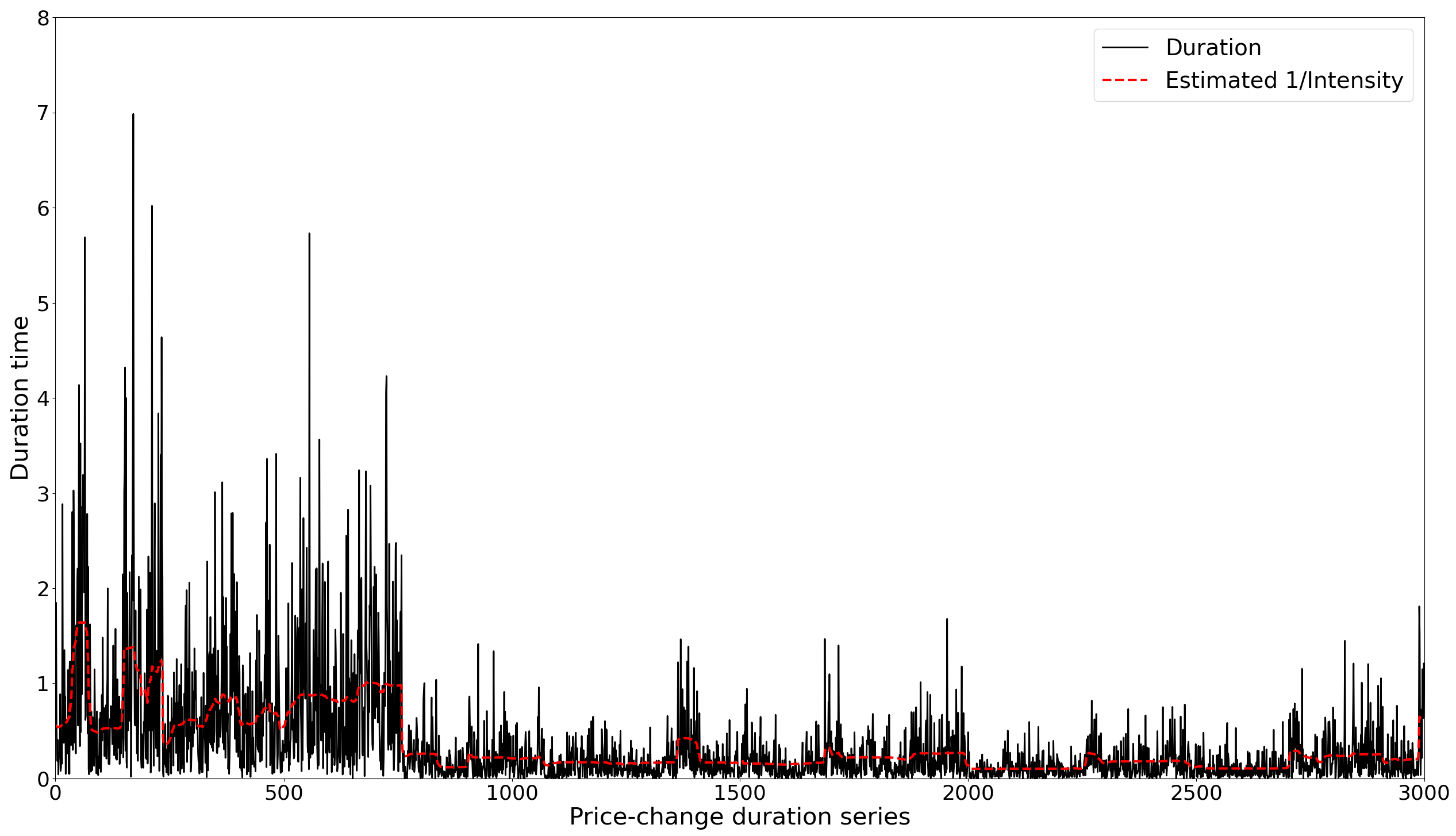
To apply our model, we construct a series of price-change durations by setting the price-change threshold. Since the minimum tick size of the simulated price is 0.01, we just set the price-change threshold for defining price durations to two ticks, i.e., δ = 0.02 . A price-change event is recorded, along with its timestamp, whenever the simulated price moves up or down by 0.02 units. The time interval between consecutive events defines the price duration. Figure 3 presents the resulting price-duration series, together with the corresponding price-change intensities estimated from the CPD model. Since long durations imply low underlying intensities, we plot the reciprocals of the estimated intensities in Figure 3 to facilitate a consistent visual comparison. The results indicate that long (short) durations are associated with low (high) price-change intensities, and that the intensities exhibit notable persistence.
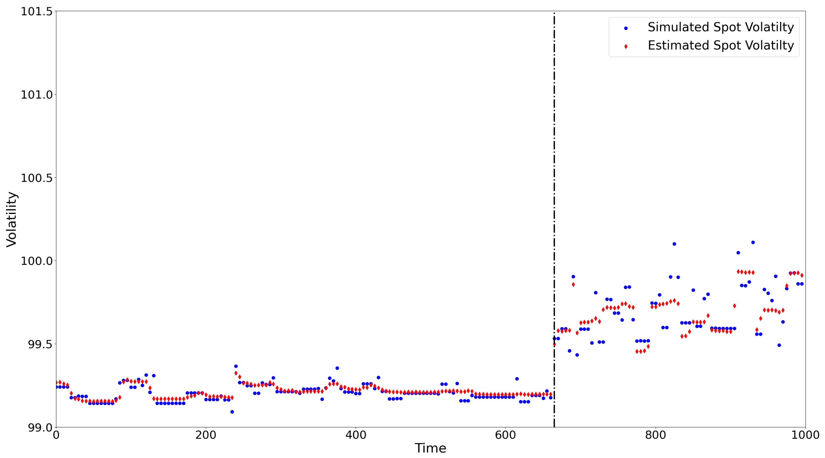
We then compute the spot volatility using Equation (6) and compare it with the true simulated volatility in Figure 4. From the results, we can find that the estimated volatility closely matches the true values. Moreover, the estimates capture the structural shift from a low-volatility regime to a high-volatility regime.

4. Real Data Analysis

4.1. Data Environment

We use Nasdaq LOB data for the real data analysis. The data are obtained from LOBSTER (https://lobsterdata.com/), which provides high-quality LOB data for all Nasdaq stocks beginning in June 2007. The LOB reconstructed by LOBSTER is based on Nasdaq’s Historical TotalView-ITCH data. For each active trading day and ticker, LOBSTER produces two files: a ‘message’ file, which records the events that trigger updates to the LOB within the specified price range, and an ‘order book’ file, which reports the state of the LOB at each update. We select 15 April 2013 for the one-day analysis because the unexpected Boston Marathon bombing significantly affected the stock market on that trading day, triggering a sharp volatility spike around the event.2 This setting provides an ideal environment to assess whether our model can capture such abrupt volatility shifts in comparison with other estimators.
Table 1 presents a sample of the message and order book files for Apple Inc. on 15 April 2013. Panel A shows five recorded events at microsecond precision. Event type 1 corresponds to the submission of a limit order, while type 4 indicates the execution of a limit order. The direction indicator ‘−1’ denotes an ask-side event, whereas ‘1’ denotes a bid-side event. Panel B displays the corresponding order book states following each event. For example, at time 34,209.630561 s (third event), the best ask order 10962867 was fully executed with the remaining size of 56 at a price of USD 426.79. After this event, the best ask shifted to the previous second-best level of USD 426.80.
Based on these two files, we can construct the price series and the price-change durations. The price is defined as the mid-price, i.e., the average of the best bid and best ask, which can eliminate the bias in duration-based estimators caused by the bid–ask spread that is mentioned in Hong et al. (2023). In practice, the choice of price-change threshold δ involves a trade-off between capturing high-frequency dynamics and mitigating noise. A larger δ produces longer durations and smoother volatility paths, but may overlook short-lived fluctuations. Conversely, a smaller δ improves granularity but may be affected by noise from bid–ask dynamics or order cancellations. As noted by Hong et al. (2023), a threshold of roughly three times the average bid–ask spread balances bias and efficiency in nonparametric estimators. In our CPD framework, bias is less of a concern since we use mid-quote prices to avoid bid–ask effects and construct durations directly from LOB data to avoid time-discretization. Accordingly, we aim to select a δ value small enough to capture granular price dynamics while relying on the change-point structure of the CPD model to filter out excess noise. For our empirical study, we set δ = 0.03 , which strikes this balance and avoids spurious price changes induced by small order cancellations.
Figure 5 plots the series of price durations for Apple stock on 15 April 2013. On that day, there are approximately 9000 durations, and the level of these price duartions shows a very large variation, with the shortest lasting 20 ms and the longest about 70 s.

4.2. Spot Volatility Measurement

We use the constructed price durations as input to the CPD model to estimate spot volatility. According to the estimation algorithm presented in Section 3.1, the parameter estimates are α ^ = 0.23 , β ^ = 0.005 , and p ^ = 0.22 . Based on Equation (15), we further infer the latent intensities { λ t } 1 N . The spot volatility σ ( t ) is then derived from Equation (6). Specifically, for t [ t i , t i + 1 ) , we have
σ 2 ( t ) = λ ( t i ) · ( δ ) 2 , t [ t i , t i + 1 ) ,
since the model assumes intensity to be constant between two consecutive events.
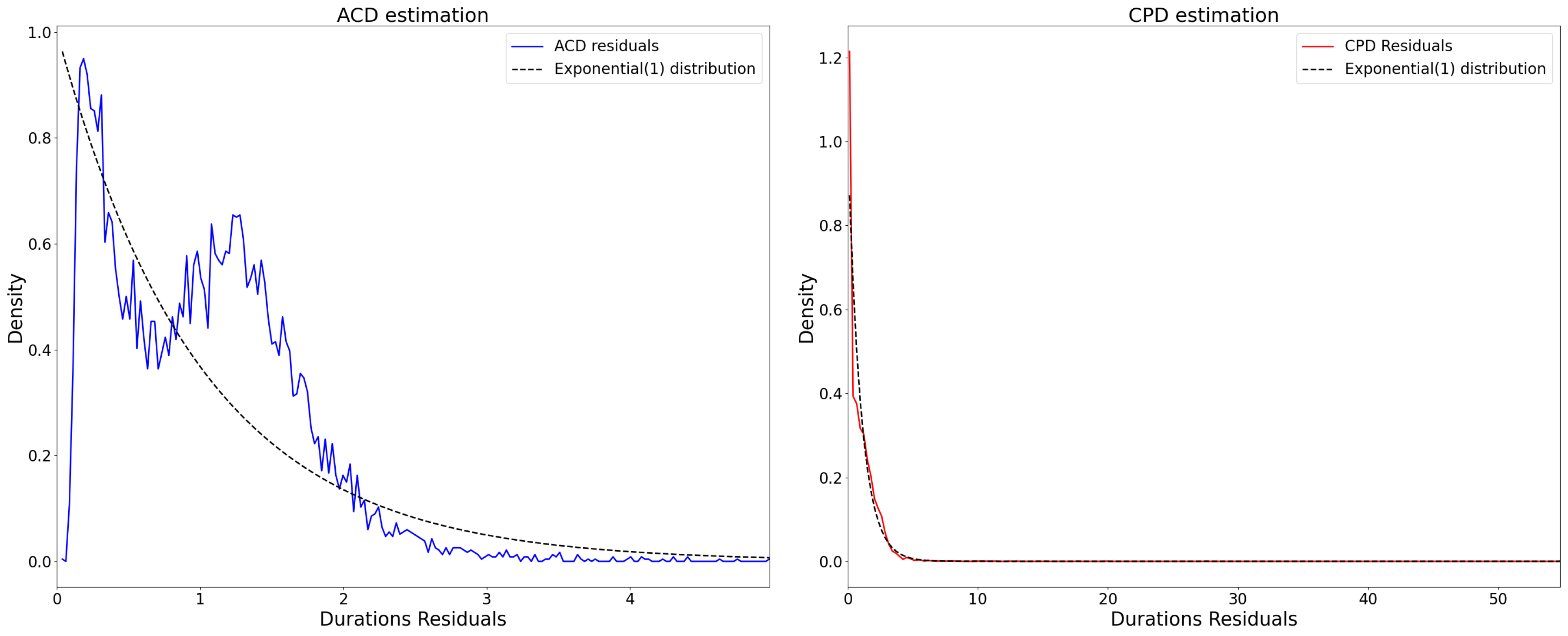
To evaluate model performance, we compare the CPD model with the classical ACD model introduced in Section 2.3. From the above discussion of the integrated intensity function (Equation (7)) and the mixture of exponential expression (Equation (8)), the estimated residuals ε ^ t should follow an Exponential ( 1 ) distribution. Figure 6 shows that the CPD model residuals adhere closely to this distribution, whereas the ACD residuals deviate substantially. This discrepancy likely arises because the ACD model cannot accommodate the large variability in high-frequency durations, which range from microseconds to tens of seconds.
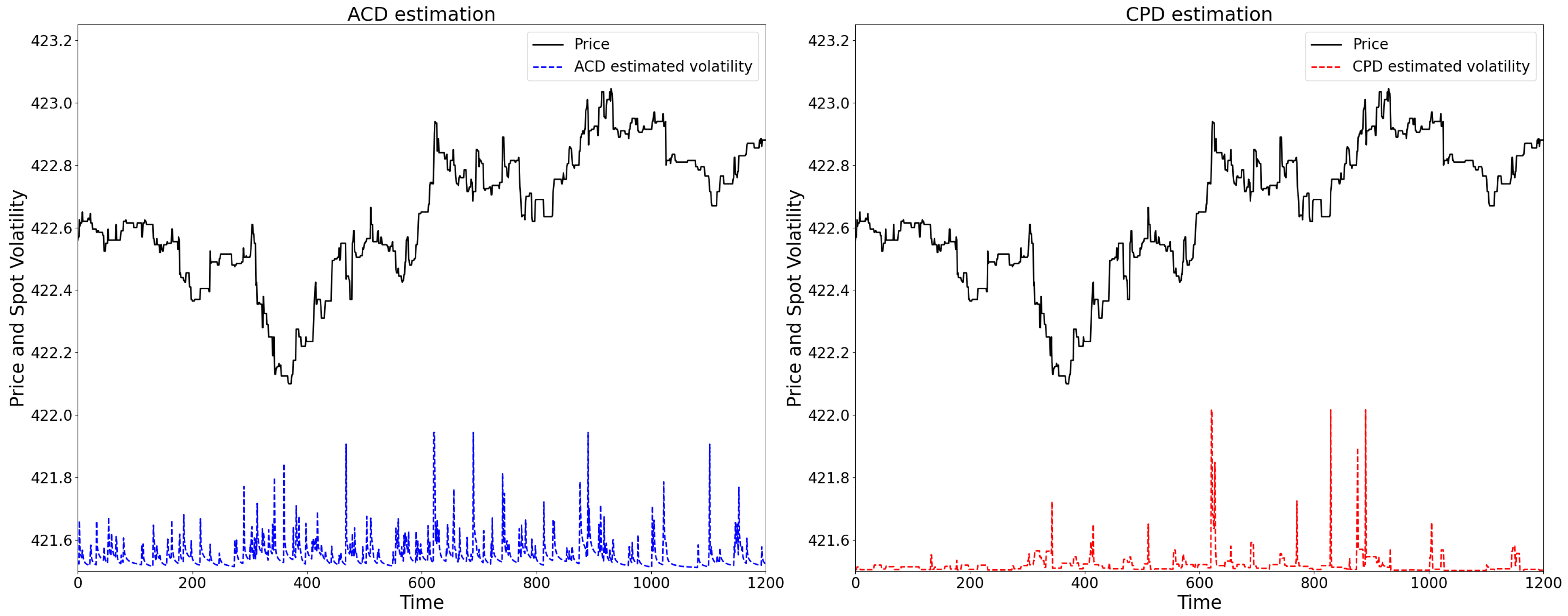
Moreover, the following Figure 7 further compares the spot volatility estimates from both models over a period of 1200 s, alongside the corresponding price data. The ACD model produces highly volatile estimates with sharp spikes whenever prices change significantly. By contrast, the CPD model generates volatility estimates that display greater persistence while still capturing abrupt price shifts.
In addition to comparing our CPD model with the standard linear ACD model, we also evaluate it against the nonlinear threshold ACD (TACD) model proposed by Zhang et al. (2001). The results are very similar and are presented in Appendix C.

4.3. Integrated Variance Measurement

The integrated variance over the interval [ 0 , t ] is as follows:
I V ( t , t + Δ t ) : = t t + Δ t σ 2 ( τ ) d W τ ,
which is the cumulative variance in returns over a time interval, providing a key measure of total risk. For portfolio managers, it quantifies exposure over the investment horizon and supports risk metrics such as Value-at-Risk. In derivative markets, it underlies option pricing through its link to quadratic variation. For high-frequency market makers, integrated variance guides bid–ask spreads and inventory control, since higher variance signals greater adverse selection risk, while lower variance allows for more aggressive quoting.
In this section, we compare the CPD model with two alternative estimators for high-frequency variance. The first is the nonparametric duration-based variance (NPDV) estimator proposed by Hong et al. (2023). It is defined over the interval [ t , t + Δ t ] as
N P D V ( t , t + Δ t ) = δ · N ( t , t + Δ t ) ,
where δ is the price-change threshold used to define events in both the CPD model and the NPDV, and N ( t , t + Δ t ) denotes the number of price-change events occurring in the interval [ t , t + Δ t ] . As shown in Hong et al. (2023), the NPDV performs comparably to parametric duration-based estimators such as the ACD model, while outperforming most of the realized variance estimators in high-frequency environments.
The second one is the optimal candlestick estimator by J. Li et al. (2024). This is designed as a nonparametric estimator of ‘spot’ volatility and given by
0.811 × ( High Low ) | Close Open | Duration of Interval ,
where ‘High’ and ‘Low’ denote the highest price and lowest price in the interval, and ‘Close’ and ‘Open’ are the closing price and opening prices in the interval. As we have mentioned in Section 2.3, this approach is limited in estimating spot volatility at very fine scales, since short intervals may not contain four distinct prices. Consequently, we apply it to construct integrated variance over relatively large intervals.
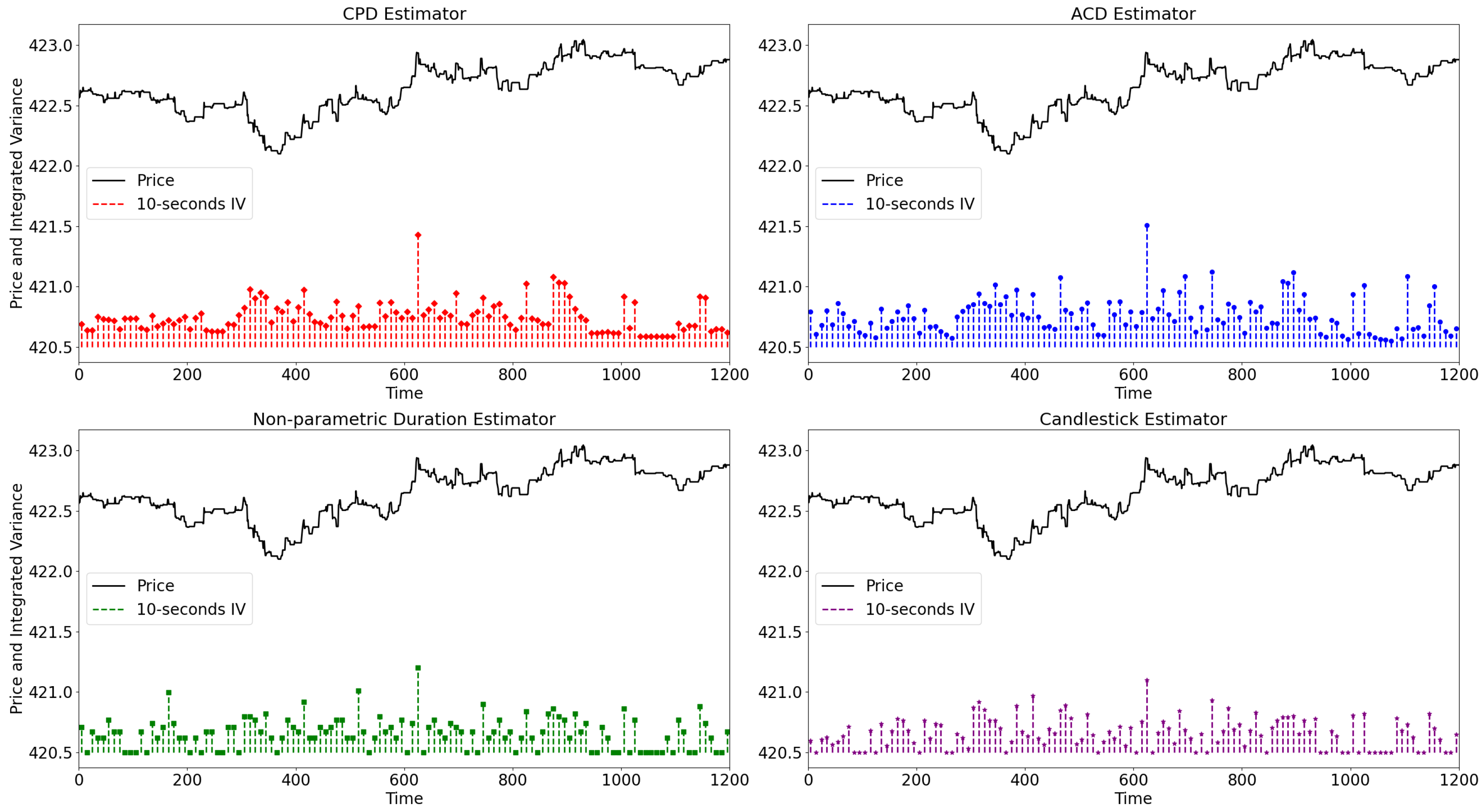
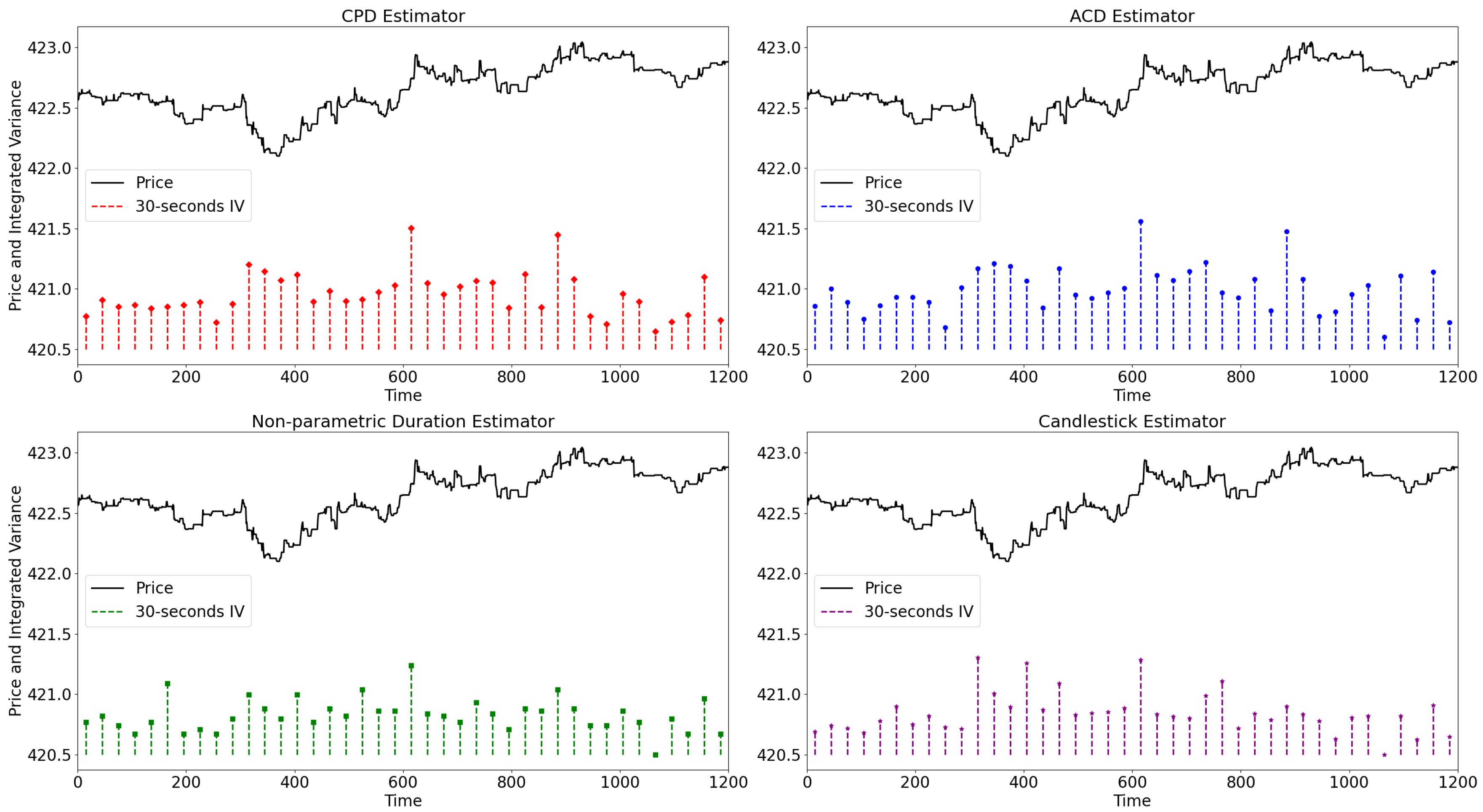
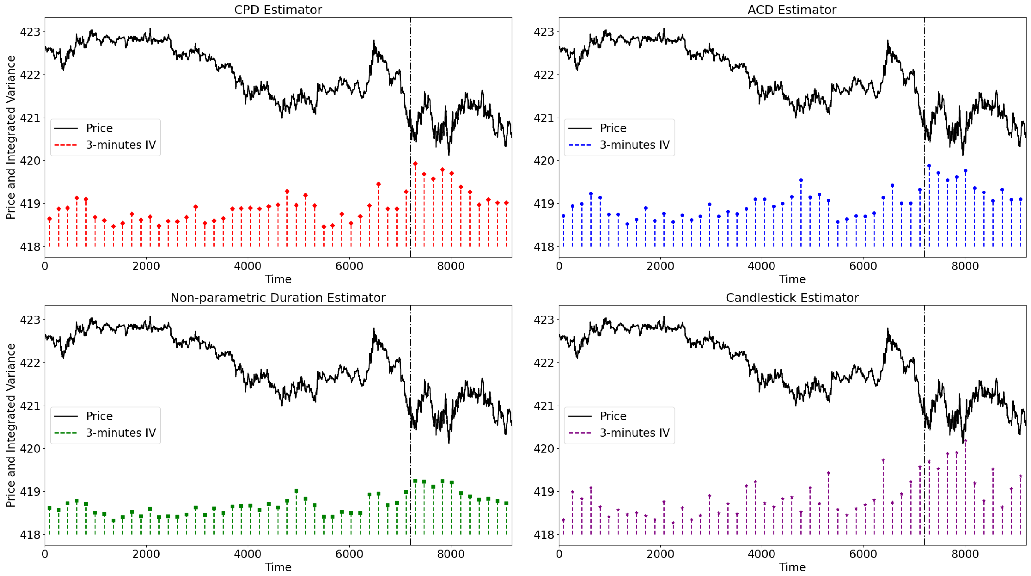
Together with the CPD and ACD models, we consider four estimators of integrated variance. Figure 8 and Figure 9 present the results for 10 s and 30 s intervals, respectively, over a 1200 s sample period. The CPD estimator produces relatively persistent variance dynamics and effectively captures volatility shifts. By contrast, the ACD estimator generates more volatile patterns with frequent sharp spikes, reflecting sensitivity to abrupt price movements. The NPDV estimator provides a stable fit but tends to understate variance in certain periods, while the candlestick estimator delivers the smoothest series but misses short-lived fluctuations due to its reliance on intraday candlestick prices. Moreover, the nonparametric duration estimator and the candlestick estimator can occasionally take the value of zero, either because no price-change events occur as defined, or because prices remain unchanged within some very short intervals. Therefore, our CPD model performs better by capturing both persistence and responsiveness in high-frequency variance estimation in these short intervals.
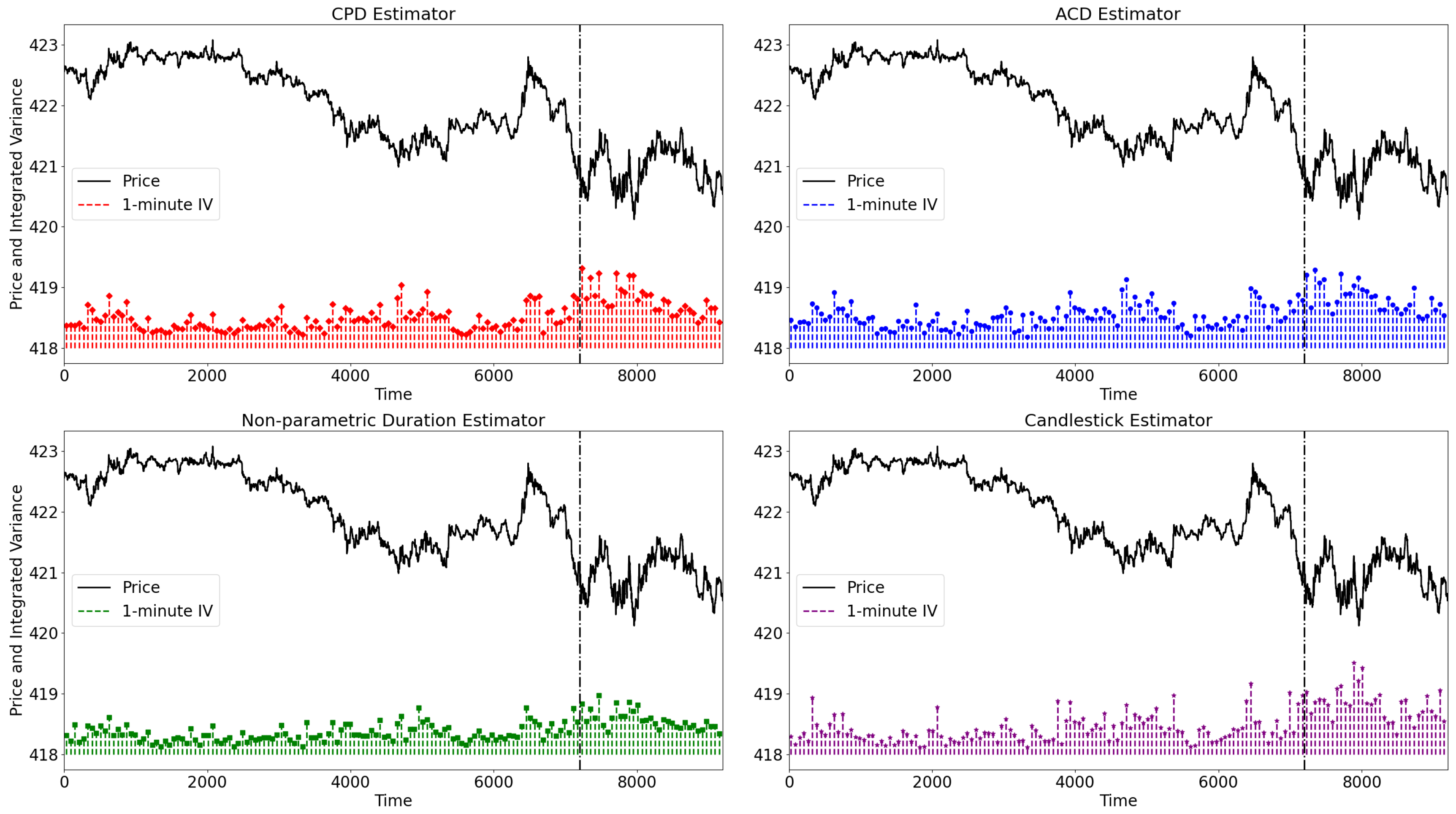
Furthermore, we estimate integrated variances over 1 min and 3 min intervals, with results shown in Figure 10 and Figure 11. To accommodate these longer horizons, the last three trading hours of 15 April 2013 are plotted, with the dashed vertical line marking the Boston Marathon bombing at approximately 3:00 PM, which triggered an immediate market shock on that day. Across all methods, a clear surge in market volatility is observed following the event, confirming the models’ sensitivity to sudden volatility jumps. The CPD estimator responds sharply while maintaining persistence, effectively capturing both the magnitude and duration of the volatility spike. The ACD estimator also detects the shock but produces noisier estimates with more fluctuations. The NPDV estimator exhibits smoother dynamics but appears to underestimate the magnitude of the shock. The candlestick estimator provides a similar patten in the low-volatility regime as our CPD model, while it fails to capture the volatility burst and decaying period following the Boston Marathon bombing. Although the nonparametric NPDV and candlestick estimator are straightforward to compute and attractive for quick, large-scale applications, they also sacrifice flexibility in capturing structural breaks or persistence in volatility. Overall, the CPD model provides the most balanced characterization of market volatility around the event.

5. Conclusions

This paper proposes the CPD model as a new framework for estimating spot volatility from price durations and demonstrates its advantages in high-frequency settings. Compared with alternative approaches such as the ACD model, the nonparametric duration estimator, and candlestick-based measures, the CPD model provides a more stable yet flexible characterization of volatility by accommodating structural breaks and sudden market shocks. Simulation results show that the CPD estimator closely tracks true volatility and captures regime shifts, while empirical analysis of Nasdaq limit order book data highlights its robustness in real markets. Particularly, it outperforms the benchmarks by capturing both persistence and responsiveness in high-frequency variance estimation in short intervals, and the application to the Boston Marathon bombing illustrates the model’s ability to detect abrupt jumps in volatility while avoiding excessive noise. The model also offers practical value for high-frequency traders and market makers, for whom accurate and timely volatility estimation is vital to managing risk, setting spreads, and maintaining profitability. Overall, this work contributes to the market microstructure literature by introducing a novel duration-based approach that links order book dynamics to volatility estimation in ultra-high-frequency settings.
Nevertheless, this study has some limitations. First, the analysis is restricted to univariate volatility dynamics, whereas multivariate extensions would be necessary to model co-movements across assets. Second, the current CPD model can identify shifts in volatility but cannot predict the direction of jumps using additional order book information. Third, estimation of the CPD model is relatively computationally intensive, which constrains its applicability for real-time market monitoring. Addressing these limitations opens up promising avenues for future research. Extensions could include multivariate CPD models for systemic risk analysis, integration with liquidity and order-flow variables, and development of real-time estimation methods suitable for live trading systems. Exploring such directions would further enhance the applicability of the CPD framework for both academic research and practical risk management in high-frequency markets.

Author Contributions

Conceptualization, Z.L.; methodology, Z.L. and H.X.; software, Z.L. and Y.W.; validation, Z.L., H.X. and Y.W.; formal analysis, Z.L.; investigation, Y.W.; resources, Z.L. and Y.W.; data curation, Z.L. and Y.W.; writing—original draft preparation, Z.L.; writing—review and editing, Y.W.; supervision, H.X.; funding acquisition, Z.L. All authors have read and agreed to the published version of the manuscript.

Funding

This research was funded by the Provincial Natural Science Foundation of Hunan Province, China, 2023JJ40191, which is acknowledged by Zhicheng Li.

Informed Consent Statement

Not appliable.

Data Availability Statement

The original contributions presented in this study are included in the article. Further inquiries can be directed to the corresponding author.

Conflicts of Interest

The authors declare no conflicts of interest.

Appendix A. Supplementary EM Steps

We refer to the our previous paper Z. Li and Xing (2022) to estimate the CPD model because the change-point structure is very similar to that work.
For the CPD model introduced in Section 2.2, the complete log-likelihood function is given by
( { y 1 n , λ 1 n } ) = log P ( λ 1 ) + t = 1 n log f ( y t λ t ) + t = 2 n log P ( λ t λ t 1 ) ,
where { y t } t = 1 n denotes the observed sequence of price-change durations and { λ t } t = 1 n the unobserved sequence of underlying intensities. Here, P ( λ 1 ) is the prior distribution of the initial intensity, f ( y t λ t ) the density of y t conditional on λ t , and P ( λ t λ t 1 ) the transition probability of λ t given λ t 1 .
In our specification, the initial intensity λ 1 is independently drawn from a Gamma distribution G ( · ) . Conditional transitions follow a Markov change-point process: with probability p, the intensity renews from G ( · ) , and with probability 1 p , it remains unchanged. Thus, the log-likelihood simplifies to
( { y 1 n , λ 1 n } ) = log G ( λ 1 ) + t = 1 n log f ( y t λ t ) + t = 2 n log G ( λ t ) · 1 ( I t = 1 ) + log p · 1 ( I t = 1 ) + log ( 1 p ) · 1 ( I t = 0 ) ,
where I t = 1 indicates that a change point occurs at the t-th trade, i.e., λ t λ t 1 . 1 ( I t = 1 ) is a indexing function that returns 1 when I t = 1 and otherwise returns 0. Similarly, 1 ( I t = 0 ) equals 1 if there is no change-point at t -th event.
In the E-step, we compute the expected log-likelihood conditional on the observed durations { y t } and the current parameter estimates. In the M-step, we update ( α , β , p ) by maximizing this expected log-likelihood. The procedure iterates until convergence, yielding both parameter estimates and posterior distributions for the latent intensities.

Appendix A.1. Expected Likelihood

In the E-step, the expected log-likelihood, conditional on D = { y 1 n , parameters   of   last   iteration } , is as follows:
E l c ( { y 1 n , λ 1 n } ) | D = E log G ( λ 1 ) | D + t = 1 n E log f ( y t | λ t ) | D + t = 2 n E log G ( λ t ) · 1 ( I t = 1 ) | D + t = 2 n log p · P ( I t = 1 | D ) + log ( 1 p ) · P ( I t = 1 | D ) ,
where the expectation is taken over the posterior distribution of hidden variables λ i .
As shown in Appendix B, the posterior distributions of λ t is as follows:
f ( λ t | D ) = 1 i t j n Π i t j · g i j ( λ t ) ,
where g i j ( λ ) Gamma ( α + ( j i + 1 ) , β + i j y t ) and Π i t j are the change-point probability that the last change point occurs at i and the next change point occurs at j + 1 , which will be calculated in Appendix B.
Moreover,
P ( I t + 1 = 1 | D ) = 1 i t Π i t t P ( I t + 1 = 0 | D ) = 1 P ( I t + 1 = 1 | D )
where t [ 1 , N 1 ] , and we also set P ( I 1 = 1 | D ) 1 .
Therefore,
E ( log f ( y t | λ t ) | D ) = λ t log f ( y t | λ t ) · f ( λ t | D ) d λ t = λ t log λ t λ t y t · 1 i t j n Π i t j · g i j ( λ t ) · d λ t
E ( log G ( λ t ) · 1 ( I t = 1 ) | D ) = log G ( λ t ) · f ( λ t , I t = 1 | D ) d λ t
Since f ( λ t | D ) = 1 i t j n Π i t j · g i j ( λ t ) , thus f ( λ t , I t = 1 | D ) = t j n Π t t j · g t j ( λ t ) . Hence, we have the following.
E ( log G ( λ t ) · 1 ( I t = 1 ) | D ) = t j n Π t t j log G ( λ t ) · g t j ( λ t ) d λ t

Maximization and the Update of Parameters

Once we have the expected log-likelihood in (A3) and write it as a function form with the following arguments ( α , β , p ) ,
l E C ( α , β , p ) E l c ( { y 1 n , m 1 n } ) | D ,
we can perform our maximization step in EM and update our estimations of model parameters.
As only the last two items in (A3) contain parameter p, therefore, by first order maximization, we have the following.
l E C ( α , β , p ) p ^ = 1 p ^ t = 2 n P ( I t = 1 | D ) 1 1 p ^ t = 2 n P ( I t = 0 | D ) = 0 ,
which gives
p ^ = t = 2 n P ( I t = 1 | D ) n 1 .
Consider items in l E C ( α , β , p ) contain parameters. It can be derived that ( α , β )
E log G ( λ 1 ) | D + t = 2 n E log G ( λ t ) · 1 ( I t = 1 ) | D = [ α log β log Γ ( α ) ] · A + ( α 1 ) · B β · C ,
where
A = t = 1 n t j n Π t t j = t = 1 n P ( I t = 1 | D )
B = t = 1 n t j n Π t t j · λ t log λ t · g t j ( λ t ) d λ t
C = t = 1 n t j n Π t t j · λ t λ t · g t j ( λ t ) d λ t .
Therefore, by maximizing (A10), we have
α ^ = C A β ^ ,
and
A · log β ^ A · ψ ( α ^ ) + B = 0 .
Thus, combining (A11) and (A12), we can solve the new value of α ^ and β ^ . In addition to the result of p ^ in (A9), we can perform the next EM iteration until the convergence of estimators.

Appendix B. The Posterior Distribution of λt in EM

Appendix B.1. Forward–Backward Filter

This section outlines the forward–backward filtering procedure for updating the posterior distribution of λ t given { y 1 , , y n } .
  • Forward Filter
Let R t = max { k I k = 1 , k t } denote the most recent change point before or at t. Given ( y 1 t , R t = s ) , the density of the posterior distribution of λ t is
g s t ( λ t ) f ( λ t | y t , R t = s ) i = s t f y i | λ t G ( λ t ) .
The posterior distribution of λ t given y 1 t can be expressed as
f ( λ t | y 1 t ) = i = 1 t p i t · g i t ( λ t ) ,
where p i t = P ( R t = i | y 1 t ) are mixture weights calculated recursively.
  • Backward Filter
Define R ˜ t + 1 = min { k I k + 1 = 1 , k t + 1 } , i.e., the next change point after t. Let q t + 1 , j = P ( R ˜ t + 1 = j | y t + 1 , n ) .
Then, the posterior distribution of λ t given y t + 1 , n is
f ( λ t | y t + 1 , n ) = p · G ( λ t ) + ( 1 p ) j = t + 1 n q t + 1 , j · g t + 1 , j ( λ t ) ,
where the weights q t + 1 , j can be obtained recursively.
  • Combination (Forward–Backward Algorithm)
The posterior distribution of λ t given the full sample { y 1 , , y n } is
f ( λ t | y 1 n ) = 1 i t j n Π i t j · g i j ( λ t ) ,
where Π i t j is the joint posterior probability of the last change point at i and the next at j + 1 .

Appendix B.2. Calculation Steps of the Posterior Intensity Distribution

In practice, the posterior intensity distribution can be evaluated as follows:
  • The conditional densities g i j ( λ ) are Gamma distributions, i.e., g i j ( λ ) Gamma ( α + ( j i + 1 ) , β + t = i j y t ) .
  • The next thing is to calculate Π i t j . By the foward–backward filter part, we can derive that Π i t j = Π i t j * 1 s t k n Π s t k * , and
    Π i t j * = p · p i t j = t , 1 i t ( 1 p ) p i t · q t + 1 , j · f i j f i t f t + 1 , j j > t , 1 i t ,
    where f i j is defined as
    f i j = t = i j f ( y t | λ ) · G ( λ ) d λ .
  • The normalizing constants f i j are obtained in closed form due to conjugacy:
    f i j = Γ ( α + j i + 1 ) · β α Γ ( α ) · ( β + t = i j y t ) α + j i + 1 .
  • The forward probabilities p i t and backward probabilities q t + 1 , j are computed recursively, which in turn yield Π i t j and hence the posterior f ( λ t | D ) .
In summary, the forward–backward algorithm shows that the posterior of λ t is a finite mixture of Gamma distributions, with weights updated recursively. This structure makes the EM algorithm computationally tractable for high-frequency data.

Appendix C. Comparison with TACD Model

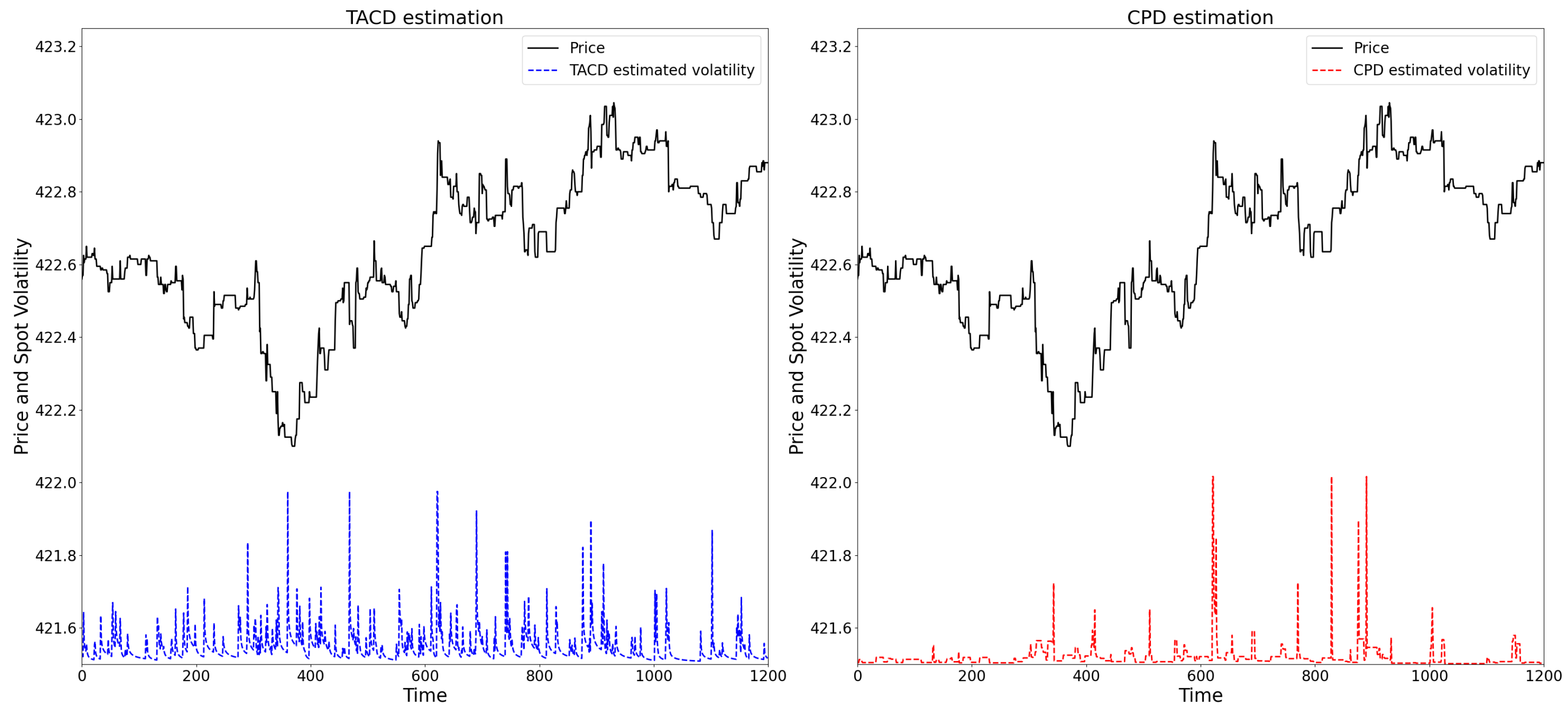
Here, we compare our model with the nonlinear threshold ACD (TACD) model proposed by Zhang et al. (2001), using the Apple LOB data from 15 April 2013. The results are plotted in the figures below. From the comparison, we can still find that (1) the residuals from the CPD model conform closely to the exponential distribution, while those from the TACD model show substantial deviations; (2) the CPD model produces volatility estimates that are more persistent and less noisy, whereas the TACD model generates highly volatile series with frequent sharp spikes; (3) the CPD-based integrated variance estimator captures structural shifts in volatility more effectively, while the TACD estimator tends to exaggerate short-term fluctuations and overreact to abrupt price changes.
Figure A1. Fitted duration residuals by TACD model and CPD model.
Ijfs 13 00186 g0a1
Figure A2. Spot volatility estimation by TACD model and CPD model.
Ijfs 13 00186 g0a2
Figure A3. Estimated integrated variance over 1 min. Vertical dashed line marks the time of Boston Marathon bombing event.
Ijfs 13 00186 g0a3

Notes

1
These approaches build on earlier work by Gallant et al. (1999) and Alizadeh et al. (2002), who introduced range-based volatility estimators for modeling and forecasting time-varying volatility.
2
Boston Marathon bombing occured on 15 April 2013. https://en.wikipedia.org/wiki/Boston_Marathon_bombing (accessed on 8 July 2025).

References

  1. Admati, A. R., & Pfleiderer, P. (1988). A theory of intraday patterns: Volume and price variability. The Review of Financial Studies, 1(1), 3–40. [Google Scholar] [CrossRef]
  2. Alizadeh, S., Brandt, M. W., & Diebold, F. X. (2002). Range-based estimation of stochastic volatility models. The Journal of Finance, 57(3), 1047–1091. [Google Scholar]
  3. Andersen, T. G., & Bollerslev, T. (1998). Answering the skeptics: Yes, standard volatility models do provide accurate forecasts. International Economic Review, 39(4), 885–905. [Google Scholar] [CrossRef]
  4. Andersen, T. G., Bollerslev, T., Diebold, F. X., & Labys, P. (2003). Modeling and forecasting realized volatility. Econometrica, 71(2), 579–625. [Google Scholar] [CrossRef]
  5. Barndorff-Nielsen, O. E., & Shephard, N. (2002). Econometric analysis of realized volatility and its use in estimating stochastic volatility models. Journal of the Royal Statistical Society Series B: Statistical Methodology, 64(2), 253–280. [Google Scholar] [CrossRef]
  6. Barndorff-Nielsen, O. E., & Shephard, N. (2004). Power and bipower variation with stochastic volatility and jumps. Journal of Financial Econometrics, 2(1), 1–37. [Google Scholar] [CrossRef]
  7. Barndorff-Nielsen, O. E., & Shiryaev, A. N. (2015). Change of time and change of measure. World Scientific Publishing Company. [Google Scholar]
  8. Bauwens, L., & Giot, P. (2000). The logarithmic ACD model: An application to the bid-ask quote process of three NYSE stocks. Annales d’Economie et de Statistique, 60, 117–149. [Google Scholar]
  9. Bollerslev, T., Li, J., & Li, Q. (2024). Optimal nonparametric range-based volatility estimation. Journal of Econometrics, 238(1), 105548. [Google Scholar] [CrossRef]
  10. Box, G. E., & Tiao, G. C. (1975). Intervention analysis with applications to economic and environmental problems. Journal of the American Statistical association, 70(349), 70–79. [Google Scholar]
  11. Cho, D. C., & Frees, E. W. (1988). Estimating the volatility of discrete stock prices. The Journal of Finance, 43(2), 451–466. [Google Scholar] [CrossRef]
  12. Daley, D. J., & Vere-Jones, D. (2003). An introduction to the theory of point processes: Volume I: Elementary theory and methods. Springer. [Google Scholar]
  13. Easley, D., Engle, R. F., O’Hara, M., & Wu, L. (2008). Time-varying arrival rates of informed and uninformed trades. Journal of Financial Econometrics, 6(2), 171–207. [Google Scholar] [CrossRef]
  14. Easley, D., Hvidkjaer, S., & O’hara, M. (2002). Is information risk a determinant of asset returns? The Journal of Finance, 57(5), 2185–2221. [Google Scholar] [CrossRef]
  15. Easley, D., & O’hara, M. (1992). Time and the process of security price adjustment. The Journal of Finance, 47(2), 577–605. [Google Scholar] [CrossRef]
  16. Engle, R. F., & Russell, J. R. (1998). Autoregressive conditional duration: A new model for irregularly spaced transaction data. Econometrica, 66(5), 1127–1162. [Google Scholar] [CrossRef]
  17. Gallant, A. R., Hsu, C.-T., & Tauchen, G. (1999). Using daily range data to calibrate volatility diffusions and extract the forward integrated variance. Review of Economics and Statistics, 81(4), 617–631. [Google Scholar] [CrossRef]
  18. Gerhard, F., & Hautsch, N. (2002). Volatility estimation on the basis of price intensities. Journal of Empirical Finance, 9(1), 57–89. [Google Scholar] [CrossRef]
  19. Glosten, L. R., & Milgrom, P. R. (1985). Bid, ask and transaction prices in a specialist market with heterogeneously informed traders. Journal of Financial Economics, 14(1), 71–100. [Google Scholar] [CrossRef]
  20. Hautsch, N. (2011). Econometrics of financial high-frequency data. Springer Science & Business Media. [Google Scholar]
  21. Hong, S. Y., Nolte, I., Taylor, S. J., & Zhao, X. (2023). Volatility estimation and forecasts based on price durations. Journal of Financial Econometrics, 21(1), 106–144. [Google Scholar] [CrossRef]
  22. Hujer, R., Vuletic, S., & Kokot, S. (2002). The markov switching acd model (Tech. Rep.). Working paper series: Finance & Accounting. Johann Wolfgang Goethe-Universität Frankfurt am Main, Fachbereich Wirtschaftswissenschaften. [Google Scholar]
  23. Lai, T. L., Liu, H., & Xing, H. (2005). Autoregressive models with piecewise constant volatility and regression parameters. Statistica Sinica, 15(2), 279–301. [Google Scholar]
  24. Li, J., Wang, D., & Zhang, Q. (2024). Reading the candlesticks: An OK estimator for volatility. Review of Economics and Statistics, 106(4), 1114–1128. [Google Scholar] [CrossRef]
  25. Li, Z., & Xing, H. (2022). High-frequency quote volatility measurement using a change-point intensity model. Mathematics, 10(4), 634. [Google Scholar] [CrossRef]
  26. Tse, Y.-K., & Yang, T. T. (2012). Estimation of high-frequency volatility: An autoregressive conditional duration approach. Journal of Business & Economic Statistics, 30(4), 533–545. [Google Scholar] [CrossRef]
  27. Zhang, M. Y., Russell, J. R., & Tsay, R. S. (2001). A nonlinear autoregressive conditional duration model with applications to financial transaction data. Journal of Econometrics, 104(1), 179–207. [Google Scholar] [CrossRef]
Figure 1. The Bayesian structure of change-point price duration model.
Ijfs 13 00186 g001
Figure 2. Simulated price and volatility under two regimes, separated by the vertical dashed line.
Ijfs 13 00186 g002
Figure 3. Simulated price durations and estimated intensities.
Ijfs 13 00186 g003
Figure 4. Simulated and estimated volatility under two regimes, separated by the vertical dashed line.
Ijfs 13 00186 g004
Figure 5. Price duration series.
Ijfs 13 00186 g005
Figure 6. Fitted duration residuals by ACD model and CPD model.
Ijfs 13 00186 g006
Figure 7. Spot volatility estimation by ACD model and CPD model.
Ijfs 13 00186 g007
Figure 8. Estimated integrated variance over 10 s.
Ijfs 13 00186 g008
Figure 9. Estimated integrated variance over 30 s.
Ijfs 13 00186 g009
Figure 10. Estimated integrated variance over 1 min. Vertical dashed line marks the time of Boston Marathon bombing event.
Ijfs 13 00186 g010
Figure 11. Estimated integrated variance over 3 min. Vertical dashed line marks the time of Boston Marathon bombing event.
Ijfs 13 00186 g011
Table 1. The sample message file and order book file of LOBSTER data.
Panel A: Message File
Time (s)Event TypeOrder IDSizePriceDirection
34,209.630122110962867100426.79−1
34,209.63045341096286744426.79−1
34,209.63056141096286756426.79−1
34,209.630623110962881100426.691
34,209.633680110962942100426.79−1
Panel B: Order Book File
Ask Price 1Ask Size 1Bid Price 1Bid Size 1Ask Price 2Ask Size 2Bid Price 2Bid Size 2
426.79100426.67100426.80100426.6212
426.7956426.67100426.80100426.6212
426.80100426.67100426.95100426.6212
426.80100426.69100426.95100426.67100
426.79100426.69100426.80100426.67100
Disclaimer/Publisher’s Note: The statements, opinions and data contained in all publications are solely those of the individual author(s) and contributor(s) and not of MDPI and/or the editor(s). MDPI and/or the editor(s) disclaim responsibility for any injury to people or property resulting from any ideas, methods, instructions or products referred to in the content.