Article

From Fields to Finance: Dynamic Connectedness and Optimal Portfolio Strategies Among Agricultural Commodities, Oil, and Stock Markets

Department of Agricultural Economics, Texas A&M University, College Station, TX 77843, USA
*
Author to whom correspondence should be addressed.
Int. J. Financial Stud. 2025, 13(3), 143; https://doi.org/10.3390/ijfs13030143
Submission received: 6 June 2025 / Revised: 28 July 2025 / Accepted: 4 August 2025 / Published: 6 August 2025

Abstract

In this study, we investigate the return propagation mechanism, hedging effectiveness, and portfolio performance across several common agricultural commodities, crude oil, and S&P 500 index, ranging from July 2000 to June 2024 by using a time-varying parameter vector autoregression (TVP-VAR) connectedness approach and three common multiple assets portfolio optimization strategies. The empirical results show that, the total connectedness peaked during the 2008 global financial crisis, followed by the European debt crisis and the COVID-19 pandemic, while it remained relatively lower at the onset of the Russia-Ukraine conflict. In the transmission mechanism, commodities and S&P 500 index exhibit distinct and dynamic characteristics as transmitters or receivers. Portfolio analysis reveals that, with exception of the COVID-19 pandemic, all three dynamic portfolios outperform the S&P 500 benchmark across major global crises. Additionally, the minimum correlation and minimum connectedness strategies are superior than transitional minimum variance method in most scenarios. Our findings have implications for policymakers in preventing systemic risk, for investors in managing portfolio risk, and for farmers and agribusiness enterprises in enhancing economic benefits.

1. Introduction

The contemporary economic landscape is profoundly shaped by the ascendancy of finance. This transformation, often termed financialization, is not a isolated phenomenon but the culmination of a systemic shift that began in the latter decades of the twentieth century. The period commonly identified as the neoliberal era is, fundamentally, an “era of finance” (Duménil & Lévy, 2004). However, over the past two decades, momentous global events have reshaped capital markets, making them more volatile than ever before. The heightened market fluctuations underscore the need for alternative assets to manage risk. Commodities such as oil, gold, agricultural products, and other metals have attracted both investors and financial institutions due to the potential for high returns, especially during periods of heightened volatility, as well as their diversification benefits in investment portfolios. In particular, the rise of Commodity Index Funds (CIFs) and Exchange-Traded Funds (ETFs) has enabled individual investors and institutional investors to gain exposure to commodities without directly engaging in the physical markets or futures contracts, accelerating the financialization of commodity markets (Cheng & Xiong, 2014). As investors flocked into these markets, commodities have transitioned from primarily physical assets traded for consumption or production to financial assets traded for speculative or investment purposes. On the other hand, the ascendancy of finance is not a phenomenon confined to Wall Street. Its connotation and practices permeated the entire economic structure, fundamentally altering the behavior of other key agents, including households and, most critically, non-financial corporations. At the company level, seeking returns from financial assets—is no longer an external pressure to which firms reacted, but a logic that had been internalized into their core corporate strategy. To individuals, they hold more diverse assets or financial or credit instruments other than stock. These shifts have rendered the correlation between commodity and equity markets more dynamic and complex, while also amplifying price fluctuations. This new market environment holds significant implications for diverse areas such as hedging practices and investment strategies.
In recent years, the relationship across crude oil, agricultural commodities, and the stock market has attracted widespread attention and discussion. The interconnection among these three markets can be attributed to several factors. On the one hand, agricultural products are used ethanol and biofuel production, and their prices are also influenced by transportation costs both of which are tied to energy prices. On the other hand, crude oil is a key input for almost all industries, and fluctuations in its price impact cash flows and production costs, which in turn can influence stock prices and overall market valuations. A large literature has identified the time-variation in the interplay between crude oil and agricultural commodity markets (Campiche et al., 2007; Chen et al., 2022; Hung, 2021; S. H. Kang et al., 2017; Wu et al., 2011; Zhu et al., 2021). The dynamic connectedness between the crude oil and stock markets have been widely reported (Chien et al., 2021; Du & He, 2015; Gatfaoui, 2016; Jebabli et al., 2022; Liu et al., 2020; Wen et al., 2012; Xu et al., 2019; Zhang et al., 2021). However, few of them have examined the linkage between agricultural commodity price and equity market. J.-S. Kang et al. (2013) identified the bilateral Granger causality behavior between international food commodity future price and Chinese stocks. Baldi et al. (2016)’s finding indicates that the connectedness between agricultural commodity and stock markets notably increased after the 2008 global financial crises which also suggests a strengthening markets interconnection.
More recent studies by Reboredo et al. (2021) examined spillovers among commodities, currencies, and major stock markets, finding that commodities, particularly, receive significant spillovers from stock markets, and in turn, affect currencies more than stocks. Hernandez et al. (2021) noted significant spillovers among agricultural commodities like grains and sugars with substantial influence on global and US stock market indices. Pinho and Maldonado (2022) highlighted the relative neutrality of agricultural markets in international emerging and developed equity markets, excluding the US. Garcia-Jorcano and Sanchis-Marco (2022) characterized significant, state-dependent tail risk spillovers across various equity indices and commodity prices, particularly during volatile periods like post-Draghi speech and COVID-19 pandemic, especially for copper and wheat. E. C. Cagli et al. (2023) observed that in the realm of agricultural commodities, agribusiness stocks act as net volatility transmitters, while the commodities themselves are net receivers. Babar et al. (2023) identified the increase of connectedness between several agricultural commodities and numerous emerging stock markets during four periods: the global financial crisis, the European debt crisis, the COVID-19 pandemic, and the Russian-Ukrainian conflict. W. Kang et al. (2023) confirmed a strong, enduring strengthening in the returns correlation between commodity and stock markets, suggesting a shift in investment capital flows within the commodity market from passive index-based strategies to more complex trading approaches.
Beyond the examination of connectedness between commodity and stock markets, considerable attention has also been given to the potential of commodities to serve as effective hedging instruments against market fluctuations. Ali et al. (2020) report that commodities can provide hedging effectiveness and exhibit a diversification potential for all groups of stock markets. Hernandez et al. (2021) show that agricultural commodities are desirable for investment, with sugar cane offering the optimal hedging effectiveness on the stock markets. Rubbaniy et al. (2022) suggests that soft commodity futures can serve as safe-haven assets for stock investment. Bunditsakulporn (2022) argue that certain agricultural commodities, such as wheat, oats, and canola, can play a safe-haven role in the Thai equity market. Mujtaba et al. (2024) find that agricultural commodities are the most suitable safe-haven assets in four commodity categories for all stock sectors in both the United States and China. Banerjee et al. (2024) indicate that containing impact investing and agricultural products in portfolios can enhance hedging effectiveness during crises.
The existing literature shows limited investigation into the connectedness of agricultural commodities (or indices) with other assets, and a distinct absence of studies exploring role of agricultural commodities in portfolio investment across prominent global crises (e.g., the COVID-19 pandemic, and the Russia-Ukraine conflict). Given the limitations of existing research, the objective of this study is to investigate the dynamics and potential portfolio implications involving agricultural commodities, crude oil, and the stock market. Specifically, we direct attention to answer the following questions:
Question 1:
Do the patterns of return connectedness behavior among agricultural commodities, crude oil, and the overall stock market vary across major global crises?
Question 2:
Do and how agricultural commodities enhance stock portfolio performance during turbulent periods?
The answers to these questions are relevant to three primary audiences. First, examining whether the linkage between agricultural commodities and stock markets evolves over time carries significant implications for policymakers and regulators. Understanding the dynamic interconnectedness among these markets may help policymakers develop strategies to shield domestic commodity markets from unintended exposures to financial volatility, alleviating the physical commodity price fluctuations that directly impact supply security and market stability. Additionally, as commodities become increasingly involved with environmental, social, and governance (ESG) considerations (E. C. C. Cagli et al., 2023; Tobler et al., 2017), insights into their interconnectedness with the stock market enable policymakers to align financial incentives with sustainability goals, directing investment flows toward environmentally sustainable and socially responsible agricultural practices. Second, individual investors and institutional funds are constantly seeking alternative assets to manage risk and evaluate whether new instruments can complement existing portfolios, particularly in increasingly volatile markets. If agricultural commodities (or indices) can reliably serve as a hedge against stock market volatility, integrating these assets into investment portfolios may help market participants diversify risk and enhance overall returns. Lastly, the third audience group includes farmers and agribusiness enterprises. With the financialization of commodities, their prices are influenced not only by traditional supply-and-demand factors but also by broader financial market turbulence. A clear understanding of the potential function of agricultural commodities in equity investments can provide valuable insights into abnormal price fluctuations in commodity markets and support remedial or preventive measures to mitigate losses. Furthermore, a strategic allocation of investments between stocks and commodities can enhance profitability for agribusinesses and individual farming operations.
In this study, we first employ the TVP-VAR and DY (Diebold & Yilmaz, 2009, 2012, 2014) spillover index model to examine the dynamic connectedness among agricultural commodities, crude oil, and the stock market. This choice is inspired by the advancements of Antonakakis and Gabauer (2017), who adeptly adapted the DY method to a TVP-VAR framework, a concept introduced by Primiceri (2005), and further developed by Antonakakis et al. (2020). The TVP-VAR structure, while maintaining the dynamic coefficients that account for changes over time, significantly enhances the original DY model. First, it demonstrates robustness to outliers, ensuring less sensitivity to extreme values in volatile financial data. Second, it obviates the need for an subjective rolling window size, thereby reducing subjectivity in the analysis. Third, it preserves all data points, preventing the loss of any observations and maximizing data utilization, allowing us to analyze and evaluate the dynamics in different sub-samples efficiently. The effectiveness and superiority of the TVP-VAR method in capturing market dynamics have been affirmed in empirical studies, including those by Antonakakis and Gabauer (2017), Korobilis and Yilmaz (2018), Antonakakis et al. (2020). Since one aim of our study is to investigate the interplay between commodities and the stock market in different periods, we avoid overly refined models to minimize the unknown disturbance from excessive parameter settings or additional modifications. Recently, the TVP-VAR models have been widely applied in the studies of the relationship among the various financial markets and the optimal allocation of assets in different scenarios (Abakah et al., 2025; Hadad et al., 2024; Han, 2025; Li et al., 2024; Sevillano et al., 2024). In second part of our analysis, we use the dynamic variance and connectedness information obtained from the TVP-VAR and DY model to build multivariate portfolios based on three optimization methods: minimum variance (MVP), minimum correlation (MCP), and minimum connectedness (MCoP). Lastly, we assess the performance of different portfolios, using a set of metrics (e.g., the hedging effectiveness, the Sortino ratio, and the Ulcer Index…) to verify the role and value of agricultural commodities within stock investment portfolios during turbulent periods.
The remainder of this paper is structured as follows: Section 2 presents the methodology, Section 3 details the data and statistical description, Section 4 discusses the results and implications, and Section 5 concludes the study.

2. Methodology

2.1. Connectedness Analysis

2.1.1. TVP-VAR Model

Diebold and Yilmaz (2009, 2012, 2014) proposed a dynamic connectedness method that captures the changes of magnitude and direction of spillover across assets or markets. With this approach, we can identify whether an asset acts as a receiver or transmitter of risk spillovers within the system. However, Antonakakis and Gabauer (2017) indicated that original connectedness approach is sensitive to the selection of rolling-window size, and it tends to overreact in the case of setting a too small one or overly smooth the effect out when the rolling-window size is too large. Korobilis and Yilmaz (2018) argued that the rolling-window estimations would exaggerate total directional and pairwise connectedness following financial crises and other notable occurrences. To overcome these limitations, Antonakakis et al. (2020); Korobilis and Yilmaz (2018) developed a Time-Varying Parameter Vector Autoregressive (TVP-VAR) model, diverging from the traditional dynamic connectedness framework.By adopting this model we can conduct a more robust analysis on patterns of connectedness behavior among agricultural commodities, crude oil, and the overall stock market across major global crises.
Now we start with modeling the commodity price changes and stock market returns as N-variable VAR(p), then the forecast error variance of variable i can be decomposed into various disturbance terms attributed to the remaining variables. That means we can determine the proportion of error variance for each variable due to shocks from others. Consider the VAR(p) with k variables,
y t = i = 1 p Φ i , t y t i + ε t
where y t = ( y 1 , t , y 2 , t , . . . , y k , t ) with each element corresponding to the returns of a specific asset, Φ represents the K × K coefficient matrix, and ε t is the error term vector. Under the assumption of covariance stationary, equation (1.1) can be rewritten in moving average form:
y t = i = 0 A i , t ε t i
where the K × K matrices A i , t follow the recursive formula A i , t = Φ 1 , t A i 1 , t + Φ 2 , t A i 2 , t + + Φ p , t A i p , t , with A 0 , t = I K × K and A i , t = 0 for i < 0 .
The TVP-VAR method extends the original connectedness approach of Diebold and Yilmaz (2009, 2012, 2014) by allowing the variance matrix to vary via a Kalman filter process in the spirit of Koop and Korobilis (2014). To illustrate the Kalman process, we further set z t 1 = ( y t 1 , y t 2 , . . . , y t p ) and B t = ( Φ 1 , t , Φ 2 , t , . . . , Φ p , t ) where z t 1 and B t represent K p × 1 and K p × K dimensional matrices, respectively. Then, the TVP-VAR(p) can be reformed as:
y t = B t z t 1 + ϵ t ϵ t Ω t 1 N 0 , Σ t vec B t = vec B t 1 + ξ t ξ t Ω t 1 N 0 , Ξ t
where the Ω t 1 denotes all information set available until t 1 , the vec B t is the vectorisation of B t which is an K 2 p × 1 dimensional vector, and ξ t also has the K 2 p × 1 form, whereas the dynamic variance matrices Σ t and Ξ t have K × K and K 2 p × K 2 p dimension, respectively. Detailed estimation process of Kalman filter are provided in Appendix A.

2.1.2. Dynamic Connectedness Indices

The variance decompositions requires the innovations to be orthogonal, however, the innovations in this VAR(p) are generally contemporaneously correlated. The standard approaches for decompositions such as Cholesky factorization are sensitive to the ordering problem (Demirer et al., 2018). For example, in Cholesky factorization, the first variable responds solely to its own shocks, and the second variable is only influenced by the impact of the first and second variables. Diebold and Yilmaz (2012, 2014) used a more generalized method to overcome this problem1, and it can produce variance decompositions invariant to ordering. Consider the H-step-ahead generalized forecast error variance decomposition matrix D i j H :
D i j H = d 11 H d 12 H d 1 K H d 21 H d 22 H d 2 K H d K 1 H d K 2 H d K K H
The element of the decomposition matrix can be denoted as
d i j , t H = σ j j , t 1 h = 0 H 1 e i A h , t Σ t e j 2 h = 0 H 1 e i A h Σ t A h , t e i , H = 1 , 2 , ,
where σ j j t is the jth diagonal element of Σ t , e i represents the selection vector with ith element equal to one and zeros for otherwise, and Σ t is the variance matrix of error term vector ε . Here, d i j , t H can be regarded as the variance contribution of variable j to that of variable i under the H-step-ahead forecasting. However, note that in generalized error variance decomposition, the sum of the standard deviation in each row, j = 1 K d i j , t H is not equal to one. Thus, d i j , t H need to be normalized as follows:
d ˜ i j , t H = d i j , t H j = 1 K d i j , t H
and then we have j = 1 K d ˜ i j , t H = 1 and i , j = 1 K d ˜ i j , t H = K . The pairwise connectedness index that measures the connectedness from variable j to variable i can be defined as:
S i j , t H = d ˜ i j , t H j = 1 K d ˜ i j , t H = d ˜ i j , t H
Generally, S i j , t H S j i , t H , thus we can further define the net pairwise connectedness index from variable i to variable j by:
S i j , t H = S j i , t H S i j , t H
In this study, the connectedness index can be used to measure the spillover among the different commodities or between commodities and portfolios. We further can obtain the total directional connectedness index which measures the connectedness to variable i from all other variables:
S i , t H = j = 1 j i K d ˜ i j , t H i , j = 1 K d ˜ i j , t H = j = 1 j i K d ˜ i j , t H K
and the corresponding total connectedness from variable i to all other variables is:
S i , t H = j = 1 j i K d ˜ j i , t H i , j = 1 K d ˜ j i , t H = j = 1 j i K d ˜ j i , t H K
Additionally, the total connectedness index (TCI) in the system can be measured by:
S T , t H = i , j = 1 i j K d ˜ i j , t H i , j = 1 K d ˜ i j , t H = i , j = 1 i j K d ˜ i j , t H K
Finally, Gabauer (2021) has introduced the pairwise connectedness index (PCI) scores that focuses exclusively on measuring the magnitude of pairwise connectedness isolating the positive and negative effects:
C i j , t H = 2 d ˜ i j , t H + d ˜ j i , t H d ˜ i i , t H + d ˜ i j , t H + d ˜ j i , t H + d ˜ j j , t H

2.2. Portfolio Analysis

2.2.1. Portfolio Optimization

To explore the role agricultural commodities play in investing, we employ three different strategies to construct our portfolios in our study. First, we adopt one of the most common method used in portfolio construction, minimum variance portfolio (MVP) approach, proposed by Markovitz (1959). This method aims to generate the portfolio with the lowest volatility based on selected assets, and the allocation weights are estimated as follows:
ω t M V P = H t 1 I I H t 1 I
where ω t is the k × 1 dimensional portfolios weights, I is a k × 1 vector of ones, and H t represents the k × k dimensional conditional variance matrix based on our TVP-VAR model. Second, we consider using another similar approach minimum correlation portfolio (MCP) procedure to build the portfolio. It was developed by Christoffersen et al. (2014) and based on the minimum conditional correlation criterion rather than minimizing the variance. We first need to calculate the conditional correlation coefficient matrix by:
R t = d i a g ( H t ) 1 / 2 H t d i a g ( H t ) 1 / 2
Then, the dynamic weights of MCP are determined by:
ω t M C P = R t 1 I I R t 1 I
Given the aforementioned two strategies, Broadstock et al. (2022) introduced a new minimum connectedness portfolio by using all pairwise connectedness indices as an alternative measure of interactions between assets. By minimizing the connectedness across assets, and thereby reducing spillovers among the system, constructs a minimum connectedness portfolio (MCoP) that is not as heavily affected by system shocks. The optimal weights for the MCoP can be defined as:
ω t M C o P = P C I t 1 I I P C I t 1 I

2.2.2. Portfolio Evaluation

To evaluate the performance of portfolios under different strategies, we adopt several metrics for comprehensive comparison. First, the hedge effectiveness introduced by Ederington (1979) is applied to compare the percentage reduction in variance of a single unhedged asset by the constructed portfolio. This hedge effectiveness (HE) is given by:
H E = H i H p H i
where H i is the conditional variance of each asset returns, and H p is the return variance of different portfolios. The higher the HE the better hedging (diversification) ability of the portfolio and vice versa.
In addition to hedging effectiveness, we also examine the time-varying cumulative returns and risk-adjusted portfolio performance for portfolios under different strategies during each turbulent periods. Specifically, we employ the Sortino ratio (Sortino & Van Der Meer, 1991), the Ulcer index (Martin & McCann, 1989), the Rachev ratio (Biglova et al., 2004), the tracking error (Roll, 1992), and the information ratio (Goodwin, 1998) to compare the performance of our portfolios across the early, middle, and late phases of different global events.
The Sortino ratio improves upon the Sharpe ratio (Sharpe, 1966) by penalizing only harmful volatility (i.e., downside deviation) rather than total volatility. It is defined as the return of the portfolio in relation to the standard deviation of negative asset returns:
S o r t i n o r a t i o = R ¯ p σ D
where R ¯ p represents the average return of portfolio, with σ D denotes the downside deviation, which measures the volatility of negative returns.
The Ulcer index measures the depth and duration a portfolio has experienced during the downside movement, and a lower Ulcer Index signifies a more stable investment with a greater resistance to deep or prolonged losses. According to Giunta et al. (2024) this index can be obtained in three steps. First, we reconstruct the portfolio price by daily returns:
P t = P t 1 1 + R p , t
where R p , t denote the returns for our portfolios, then we consider a period of T, and define drawdown as:
d d t = P t max 1 τ t P τ max 1 τ t P τ , t = 1 , 2 , , T
Finally, the Ulcer index can be expressed in:
U l c e r i n d e x = t = 1 T d d t 2 T
The Rachev ratio is a risk-adjusted performance measure specifically designed to evaluate assets with non-normal, or “fat-tailed” return distributions. A higher Rachev ratio indicates the potential for upside gains outweighs the potential for downside losses. It can be defined as:
R a c h e v r a t i o = C V a R α ( R p , t ) C V a R β ( R p , t )
where conditional value-at-risk C V a R α represents the average loss in the worst α % = 5 % of cases, and C V a R β is the average return in the best β % = 5 % of cases.
Tracking error, or more precisely, tracking error volatility, refers to the residual risk or the volatility of the excess returns. It measures how closely a portfolio follows its benchmark, providing an estimate of the active risk for portfolios. A lower tracking error indicates that the portfolio closely follows the benchmark, whereas a higher value suggests greater deviation and active management. It can be obtained by:
T r a c k i n g e r r o r = 1 n 1 t = 1 n R p , t R b , t 2
where R b , t denote the returns for the benchmark.
Building on tracking error, the information ratio is used to evaluate how efficiently a portfolio generates excess return for each unit of risk, with higher values indicating greater consistency and skill in outperforming the benchmark, and is defined as follows:
I n f o r m a t i o n r a t i o = R ¯ p R ¯ b T r a c k i n g e r r o r

3. Data

In our dynamic connectedness analysis, we use the daily S&P Goldman Sachs Commodity Indices (GSCI). These non-seasonally adjusted and tradable indices are readily available to market participants. The data span from July 2000 to June 2024, and are sourced from Refinitiv Eikon, ensuring both reliability and accuracy. This timeframe encompasses the pivotal period of commodity financialization that began in the early 2000s, covering multiple major global crises. By including these distinct crisis periods alongside pre-crisis baselines and post-crisis adjustments, the chosen timeline facilitates a robust investigation into how the dynamic connectedness between agricultural commodities, crude oil, and the stock market evolves under varying economic and geopolitical conditions. Specifically, we select a comprehensive set of agricultural commodity indices, including three grains (corn, soybeans, wheat), two softs (cotton, coffee), one commodity (live cattle), and crude oil. The rationale for selecting these commodity indices is multi-faceted: (1) it is one of the most widely accepted and inclusive benchmark, weighted by production, that captures the global market beta; (2) the index is constructed to be investable by incorporating the most most actively traded commodity futures, and avoids to accounting for varying maturities and expiration times; (3) daily data can provide timely perspective, discerning immediate market movements and economic trends, and help minimize the noise and improve the signal-to-noise ratio, which is particularly important in volatile financial markets (Claessens & Schmukler, 2007; Rubbaniy et al., 2024); (4) by taking crude oil price as a proxy for the heterogeneity, the model can link the agricultural commodity market and the stock market more closely. We use S&P 500 index to represent the overall stock market.
Table 1 summarizes the descriptive statistics for the daily logarithmic returns of S&P 500 and spot commodity indices for the full sample. Despite the average returns for all assets being close to zero, there are some notable outliers. For instance, the largest positive ( 43.79 % ) and largest negative ( 56.86 % ) returns were observed for the crude oil spot index. By skewness statistics, negative tail asymmetries are observed in most assets, excluding wheat and coffee, which are positive tail asymmetrical. The kurtosis statistics show that most return series follow leptokurtic or platykurtic distributions with the the sole exception of coffee. The Jarque-Bera tests reinforce the fact that no return series is normal distributed. According to the Ljung-Box Q(20) and Ljung - Box Q 2 ( 20 ) tests, we can see that most return series exhibit autocorrelation and ARCH/GARCH error effects are significantly identified Finally, the augmented Dickey-Fuller (ADF) test confirms that all series are stationary. In general, the statistics in Table 1 support our decision to use the TVP-VAR method for the analysis of dynamic connectedness between the commodities and equity market.
Figure 1 depicts the Pearson correlation coefficient matrix of S&P 500 and spot commodity indices for the entire sample. It can be seen that S&P 500 has small and positive correlations with various agricultural spot commodity indices, meaning that those commodity indices may be used as diversification for stock market investment. Notably, grains exhibit the largest correlations among all assets, while the correlations of livestock commodity are much less than those of others. This matrix also reflects the clear clustering of agricultural commodities into grains, softs, and livestock. Interestingly, crude oil exhibits behavior that is relatively more aligned with the characteristics of soft commodities.
To study the impact of turbulent events on the dynamic relationship among these commodities and the U.S. stock market, we divide our dataset into four sub-periods: (1) the first one is the 2008 global financial crisis (3 December 2007–30 June 2009); (2) the second series corresponds to the European debt crisis (3 May 2010–31 May 2012); (3) the next period is for the COVID-19 (1 January 2020–31 December 2021); (4) the last one is regarding the first round of invasion and counteroffensive in the Russia-Ukraine conflict (1 February 2022–11 November 2022).

4. Results and Discussion

4.1. Connectedness Analysis

4.1.1. Static Connectedness

Table 2 shows the average connectedness among the agricultural commodity indices and the stock market returns. We obtain our connectedness results through the TVP-VAR model with a lag order of one, according to the Bayesian Information Criteria, along with a 5-step-ahead (one week) generalized forecast error variance decomposition. In Panel A of Table 2, the i j th entry represents the contribution to the forecast error variance of market i coming from innovations to market j. For example, the 19.39 in the first row from Panel A means that innovations to the soybeans return are responsible for 19.39 % of the error variance in forecasting the 5-day-ahead corn price change. And we can see the return spillover from soybeans to corn is smaller than for the corn to soybeans ( 21.04 % ). The diagonal elements estimate their own variance shares, which represent the fraction of the forecast error variance of market i that is attributed to its own shock. Furthermore, the off-diagonal row sums in the column labeled “FROM” are the directional connectedness from other remaining markets to the market in each row. Analogously, the off-diagonal column sums of the row labeled “TO” represent the directional connectedness from each market in each column to the other remaining markets. “NET” in the last row for each asset is the difference between the total connectedness from one market to others and the total connectedness from others to this market. “TCI” located in the lower right corner of each panel is the total connectedness index, which measures the percentage of the total of off-diagonal row sums (or column sums) relative to the total row sums (column sums) including the diagonals (the spillovers from or to their own). “cTCI” is the corrected total connectedness index, which is adjusted by multiplying TCI by k 1 / k . It is worth highlighting again that all the numbers in Table 2 reflect the average values over the corresponding period.
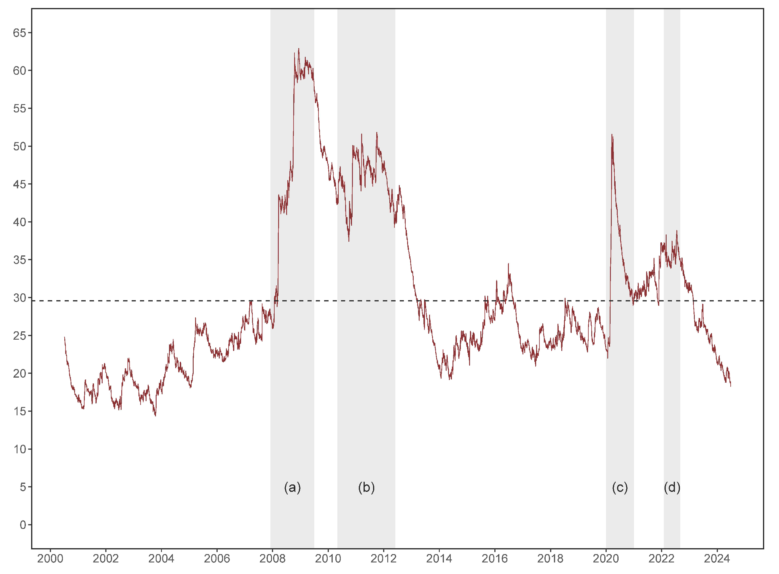
In Panel A of Table 2, the TCI for the entire sample is 29.40 % , indicating the moderate interconnectedness within the system, since on average only 29.40 % of the forecast error variance in one commodity class or overall stock market can be associated with return innovations (shocks) from other assets. The average connectedness results for the subsample periods presented in Panels B to E of Table 2 all exhibit varying degrees of increase, suggesting that return spillover effects tend to intensify during turbulent periods. Specifically, the average TCI value reached its highest level during the 2008 financial crisis, peaking at a value of 52.60 % , followed by the European debt crisis period ( 43.21 % ). The lowest average system connectedness was observed during the COVID-19 pandemic ( 32.22 % ), although it is similar to that of the Russia-Ukraine conflict ( 35.03 % ). While the above analysis provides information on the “average” return connectedness information, it may overlook market dynamics or cyclical movements in associated with global events. To examine how, and to what extent, these events trigger deviations from the average TCI, we plot the daily connectedness in Figure 2 based on our TVP-VAR framework, illustrating the evolution of systemic connectedness.

4.1.2. Dynamic Total Connectedness

According to the results in Figure 2, the total connectedness within network varies considerably over the full sample time, ranging from 13.13 % to 62.16 % . It can be observed that, prior to the 2008 financial crisis, the TCI consistently remained below its average level, staying under 30 % . Beginning in the late 2007, as the global financial crisis took shape, connectedness rose sharply, peaking at 62.16 % . Following the end of the economic recession, systemic TCI start to decline until the onset of the European debt crisis, during which it remained elevated, fluctuating between 37 % and 51 % . After the resolution of this crisis, the TCI decreased once more, eventually returning to pre-2008 financial crisis levels. It should be noted that between 2014 and 2016, connectedness experienced a period of sustained moderate increase, coinciding precisely with the collapse of global oil price. Given that the crude oil price is used to bridge commodity and stock markets within our analytical framework, this observation appears reasonable. The connectedness steadily hovered at lower levels until the first half of 2020, when it sharply rose to the high levels comparable to those observed during the European debt crisis, coinciding precisely with the first wave of COVID-19 outbreak. After this spike, the connectedness rapidly returned to its average level by the end of 2020. In February 2022, following the onset of the Russia–Ukraine conflict, the TCI increased from average level to 36 % , and subsequently declined to 19 % by the end of data. The evolving trend is in line with the findings of Babar et al. (2023) regarding the relationships between agricultural commodities and multiple emerging stock markets.
Besides the total connectedness, it is also useful to know the individual asset directional connectedness, particularly the to-degrees, as we are interested in identifying which assets send the most uncertainty to others. In Panel A of Table 2, corn with a to-degree of 57.32 % , is the commodity that contributed the largest percentage of shocks to other markets over the full sample. The next two highest contributors are soybeans and wheat, with to-degrees of 47.60 % and 42.65 % , respectively. Notably, live cattle has the lowest to-degree ( 10.31 % ) meaning it contributes the least impact of shocks to other commodities and the stock market, followed by coffee ( 15.23 % ). Regarding the stock market, its to-degree is smaller than that of grains, cotton, and crude oil. In contrast, the from-degree directional connectedness among assets exhibits a narrower range, varying from a high of 49.13 % (corn) to a low of 13.24 % (live cattle). Although the general clustering ranks for both to-degree and from-degree directional connectedness are similar, the to-degree ordering does not exactly match the from-degree ordering. From the results of remaining panels of Table 2, we can see the behaviors of directional connectedness vary across different sub-sample periods.
Based on directional connectedness, we can use the difference between the to-degree and from-degree connectedness to identify the role of each asset within the network. Those assets with positive net connectedness values are more likely to transmit shocks to others than to receive shocks from external sources, whereas assets with negative net connectedness are more easily affected by others, while their transmission of shocks to others is relatively small. In Panel A of Table 2, only corn and soybeans provide positive average net connectedness values over the full sample period. Specifically, commodities contributing the top three net impacts to others are corn ( 8.19 % ), soybeans ( 3.01 % ), and wheat ( 0.01 % ), while coffee ( 3.65 % ), cotton ( 3.02 % ), and live cattle ( 2.94 % ) exhibit the most negative net connectedness. The dominant role of grain commodities is consistent with the findings of Hernandez et al. (2021) in the context of global equity markets. This result is not surprising, given that grain commodities are not only important consumption items for households globally, but also serve a critical function in the production of biofuel.

4.1.3. Sub-Sample Connectedness Network

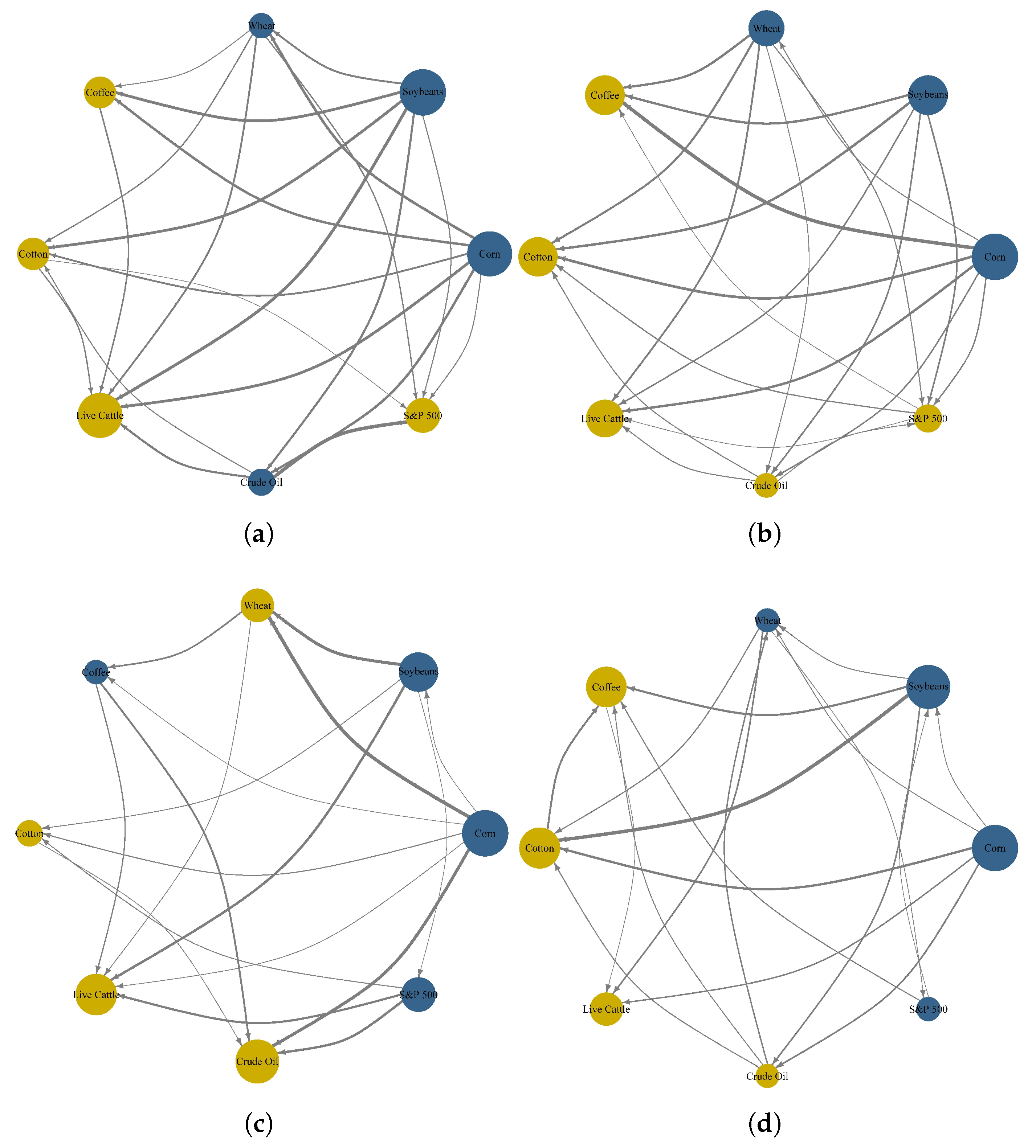
Although the aforementioned connectedness results are quite valuable in identifying the dynamic changes of the entire system, they fall short in capturing pairwise dynamics, particularly the pairwise (or bilateral) connectedness between each commodity and the stock market. Given the aim of our study, understanding these dynamics are necessary to provide a clearer perspective on the role commodity plays in relation to stock market within our network. Accordingly, we present the results of net pairwise connectedness to further elucidate the linkages across the different commodity markets of our interest. Figure 3 provides a visually accessible depiction of average net pairwise directional connectedness among all sampled commodities and the S&P 500 during the different sub-sample periods. The color and size of the nodes indicate whether the commodity or the stock market acts as a transmitter (blue) or receiver (yellow) and average weighted connectedness, while the direction and thickness of the arrows between the nodes represent the magnitude of the connectedness, complementing the findings shown in Figure Table 2.
We observe that, in our network, corn and soybeans consistently act as transmitters of spillover effects, while cotton and live cattle are always influenced by other markets. In contrast, the color changes of nodes suggest that other commodities (wheat, coffee, and crude oil) and the S&P 500 shift between being receivers and transmitters of shocks within network across different periods. Extending the work of Hernandez et al. (2021) we confirm the shifting roles of commodities and equities across different periods. Particularly for the stock market we focus on, compared to the financial crisis when the S&P 500 acted as a receiver, it transitioned to a transmitter during the pandemic and Russia-Ukraine conflict periods. One possible explanation for this change could be the ongoing financialization of agricultural commodities, which has made their prices or indices more sensitive to shocks originating from financial markets than ever before. Additionally, we find that the network connectedness is more intricate in financial crisis. The reason behind this phenomenon may lie in the fact that the public health events and geopolitical tensions exert more influence on commodity markets rather than stock market, thereby weakening the overall connectedness effects.

4.1.4. Dynamic Pairwise Connectedness

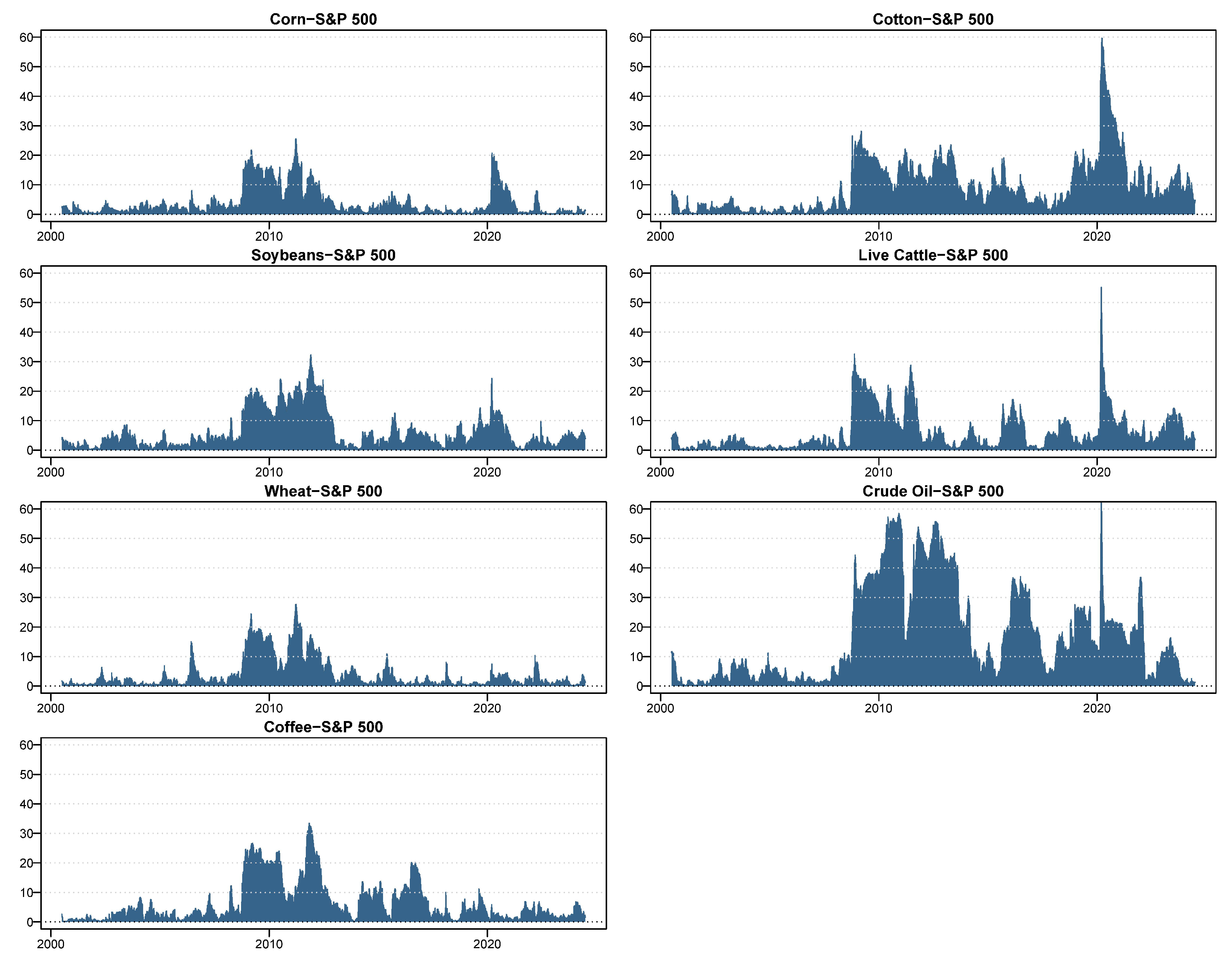
Unlike Table 2 and Figure 3 which identify the roles of spillover transmitters or receivers, Figure 4 focuses exclusively on measuring the magnitude of pairwise connectedness between the S& P 500 and commodities using a standardized index score. This index score, ranging from 0 to 100, mitigates the disturbances caused by shifts between transmitter and receiver roles, offering a clearer depiction of changes in pairwise connectedness throughout the entire cycle. We can see that the connectedness between commodities and the stock market strengthened after the 2008 financial crisis. It is not surprising that the connectedness of crude oil with the stock market is stronger than that of other commodities, given that oil prices to some extent capture the economic performance and expectations regarding economic growth.
Taken as a whole, our connectedness results provide evidence in response to our first research question, suggesting that return connectedness among agricultural commodities, crude oil, and equity markets varies over time and exhibit distinct patterns across different sub-periods. In particular, the connectedness level peaked during the 2008 global financial crisis, surpassing levels seen in other periods. Although the European debt crisis and the COVID-19 pandemic exhibited similarly elevated peaks, the former was more prolonged, while the latter experienced a swift decline. Within the four sub-sample intervals, the lowest levels of connectedness is observed during the Russia–Ukraine conflict. Notably, the wheat, coffee, crude oil and the S&P 500 shift between being receivers and transmitters of shocks, emphasizing the evolving roles of amid episodes of market turbulence.

4.2. Dynamic Portfolios

In this subsection, we turn to the portfolio performance of three diversification hedging strategies, to further evaluate how agricultural commodities can contribute to improving investment efficiency and mitigating stock market risk. First, we compare the cumulative returns of our three technical portfolios and the S&P 500 index investment across four subsample periods. Then, we provide the dynamic optimal weights of each asset in multivariate portfolios under the three strategies. Finally, we assess the hedging effectiveness and risk-adjusted performances of the portfolios during turbulent periods.

4.2.1. Cumulative Returns

Figure 5 presents the cumulative returns of multivariate portfolios combined with the unhedged S&P 500 index as benchmark in times of market turbulence. We can see that the overall trends in cumulative returns across all portfolios are consistent during turbulent periods, and our multivariate portfolios outperform the unhedged S&P 500 index investment (excluding the pandemic episode). The weaker performance of diversified portfolios compared to the standalone S&P 500 index during the pandemic period can be largely attributed to the unique nature of public health crises and aggressive market rescue measures. During the COVID-19, sharp declines in commodity prices were driven by sustaining disruptions in global demand and supply chains issues. Conversely, under the unprecedented monetary policy actions by the Federal Reserve (cutting interest rates to near-zero level and extensive quantitative easing), the S&P 500 experienced the rapid and robust rebound, showing dramatic returns that outpaced the recovery in agricultural commodity prices.
The figure also compares the performance of three different portfolio allocation strategies. In Figure 5, we can see that the MCP and MCoP outperform in the first half of the 2008 global financial crisis, the European debt crisis, and the Russia-Ukraine conflict, whereas in the latter half of each period, their cumulative returns gradually converges with that of the MVP, reaching an equivalent level by the end. During the COVID-19 pandemic, we also find that the performance of the MVP is overall superior to that of the MCP and MCoP. Notably, our MCP and MCoP strategies exhibit a visible level of overlapping in cumulative returns. This similarity is not surprising, since MCP and MCoP are both constructed based on the derivation from the same time-varying variance matrix.

4.2.2. Dynamic Allocation Weights and Hedging Effectiveness

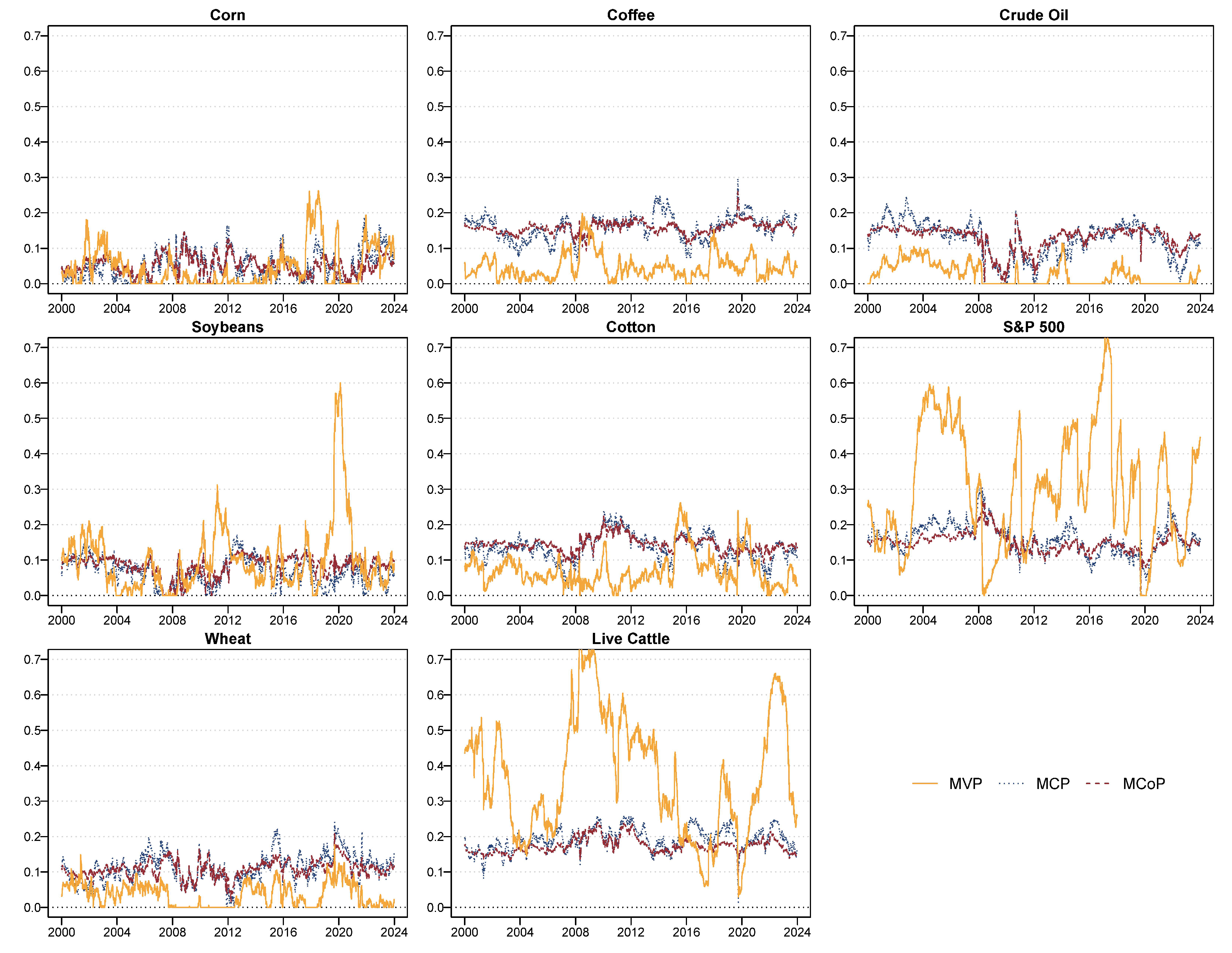
To explore assets allocations in three portfolios, we provide the results of optimal weights over the full sample period in Figure 6. It is clear that the optimal portfolio weights under three strategies exhibit time-varying characteristics. The weights allocated by the MVP differ substantially from those of the other two portfolios, sharing more fluctuation, while the weights of the MCP and the MCoP are similar to each other, echoing the comparable trajectories of cumulative returns generated by MCP and MCoP. Notably, under the MVP approach, live cattle and the S&P 500 are alternately assigned weights significantly higher than those of other assets. A plausible explanation for why live cattle receives higher weights is that its price volatility is substantially lower than that of other agricultural commodities. Consequently, in the minimum variance portfolio, it contributes more to reduce overall portfolio volatility, particularly during turbulent periods.
In Table A1, we provide more concrete description of the dynamic optimal weights, as well as the hedging effectiveness of the three portfolios across different periods. We first look at Panel A of Table A1, it presents the mean, 5 % / 95 % percentiles, and the standard deviation of the optimal weights, as well as the hedging effectiveness that the portfolios provide for each asset. Taking the MVP for example, the average optimal weight corresponding to corn is 0.02 over the 2008 global financial crisis, and this value indicates that for a $100 budget combination of S&P 500 and commodities multivariate portfolio $2 should be invested in corn, while the remaining dollars allocated in other assets. The 5 % / 95 % percentiles and the standard deviation are derived from the daily frequency outputs of the optimal portfolio weight and also confirm the evolving features of the hedging strategies.
The hedging effectiveness results indicates that if a portfolio is constructed based on the assets (e.g., corn, soybeans…) and corresponding weights shown in Panel A of Table A1, as a result, the volatility of each asset in this portfolio would be reduced by 84 % , 82 % …, respectively. We can see that in minimum variance strategy, live cattle is assigned the highest average weight, while wheat and crude oil contribute minimally. In minimum correlation and minimum connectedness portfolios, the budget are allocated more evenly to various assets. Regarding the hedging effectiveness results, the MVP provides reductions in volatility ranging from 74 to 92 % , excluding live cattle ( 13 % ), whereas the performance of the MCP and MCoP is slightly weaker. In general, the hedging effectiveness of the portfolios for each asset is similar across the three strategies. It should be mentioned that the portfolio hedging effectiveness against to live cattle is negative in MCP and MCoP, which suggests that the volatility of returns of live cattle is smaller than those of two multivariate portfolios. This pattern is not observed in the MVP, as the assets share allocated to live cattle in MCP and MCoP is comparatively lower. Across all three strategies, livestock commodities receive the highest weights, followed by soft commodities, then grain commodities, while the role of crude oil is negligible. In line with Ali et al. (2020) and Mujtaba et al. (2024), our findings reaffirm that agricultural commodities serve as effective hedging tools and provide diversification benefits for stock market investments.
Comparing the hedge effectiveness of our portfolios across the sub-sample periods, we find that our portfolios performed better during the 2008 financial crisis and the Russia-Ukraine conflict than during the European debt crisis and the COVID-19 pandemic. Upon closer examination, the performance of the three portfolios is not consistently aligned across each turbulent periods. In most cases, the MVP strategy offers superior hedging effectiveness for assets than other two strategies, with the variations being most pronounced during the European debt crisis and the COVID-19 pandemic. These differences may be attributed to several aspects, including evolving market dynamics and commodities-specific behavior unique to each global event. For example, the lockdowns imposed during the pandemic led to a decline in agricultural commodity prices, whereas the Russia-Ukraine conflict triggered sharp increases in those prices. The markedly different price trajectories across periods influenced the effectiveness of agricultural commodities as hedging instruments.

4.2.3. Risk-Adjusted Portfolio Performance

Table 3 examines the risk-adjusted performance of our portfolios. We use several evaluation metrics to assess whether the portfolios outperform the unhedged benchmark. Specifically, we report the performance of three portfolio as well as the S&P 500 across different turbulent periods, further dividing each period into early, middle, and late stages. We find that, except the COVID-19 period, the multivariate portfolios outperform the unhedged S&P 500 in the early stages of each sub-period, which is consistent with our earlier findings based on cumulative return performance.
Specifically, the higher Sortino ratio for three portfolios suggesting the superior performance of these strategies during the early stage of crises. However, for the COVID-19 pandemic scenario, our three portfolios perform better in the middle and late phases rather than early one. The lower Ulcer index than that of the S&P 500 also indicates that these portfolios experienced very shallow and brief periods of loss and not fallen far from its previous peaks. As for Rachev ratio, our portfolios beat the S&P 500 with greater potential for extreme positive returns compared to the risk of extreme negative returns. The tracking error results show the degree to which various strategies track the benchmark does not exhibit significant variation across different periods and phases. Notably, in Panel C of Table 3, we can see that in the early stage of the pandemic, the tracking error relative to the S&P 500 reaches 3.0635 , markedly exceeding levels observed in other periods and phases. It means that the portfolio deviated significantly from the S&P 500. As for information ratio, except for the COVID-19 and the MVP, the results are identical with those of Sortino ratio, Ulcer index, as well as Rachev ratio, robustly confirming the strong performance of the portfolio in the early stage.
In addition, the table also provides useful information to evaluate the portfolio performance across three different allocation strategies. By comparing the performance of various portfolios at different crises and stages, we find that: during the 2008 financial crisis, the European debt crisis, and the Russia–Ukraine conflict, MCP and MCoP generally outperformed MVP across all stages. In contrast, amid the COVID-19 pandemic, MVP performed better than the other two portfolios.
Overall, our results suggest that incorporating agricultural commodity indices into stock market investment portfolios can offer significant hedging effectiveness during turbulent periods, reducing the volatility of asset returns, which are financially meaningful in risk management. Specifically, we find that hedging effectiveness is higher during the 2008 financial crisis and the Russia-Ukraine conflict compared to the European debt crisis and the COVID-19 pandemic. During market turmoil (excluding the pandemic episode), the results of risk-adjusted portfolio performance suggest that the minimum correlation and the minimum connectedness portfolios generate better risk-adjusted returns performance in the early phases of crisis periods. Notably, throughout the COVID-19 pandemic, the MVP strategy outperforms the other portfolios, with all three strategies exhibiting stronger risk-adjusted performance in the middle and late phases compared to the early phase.

4.2.4. Robustness

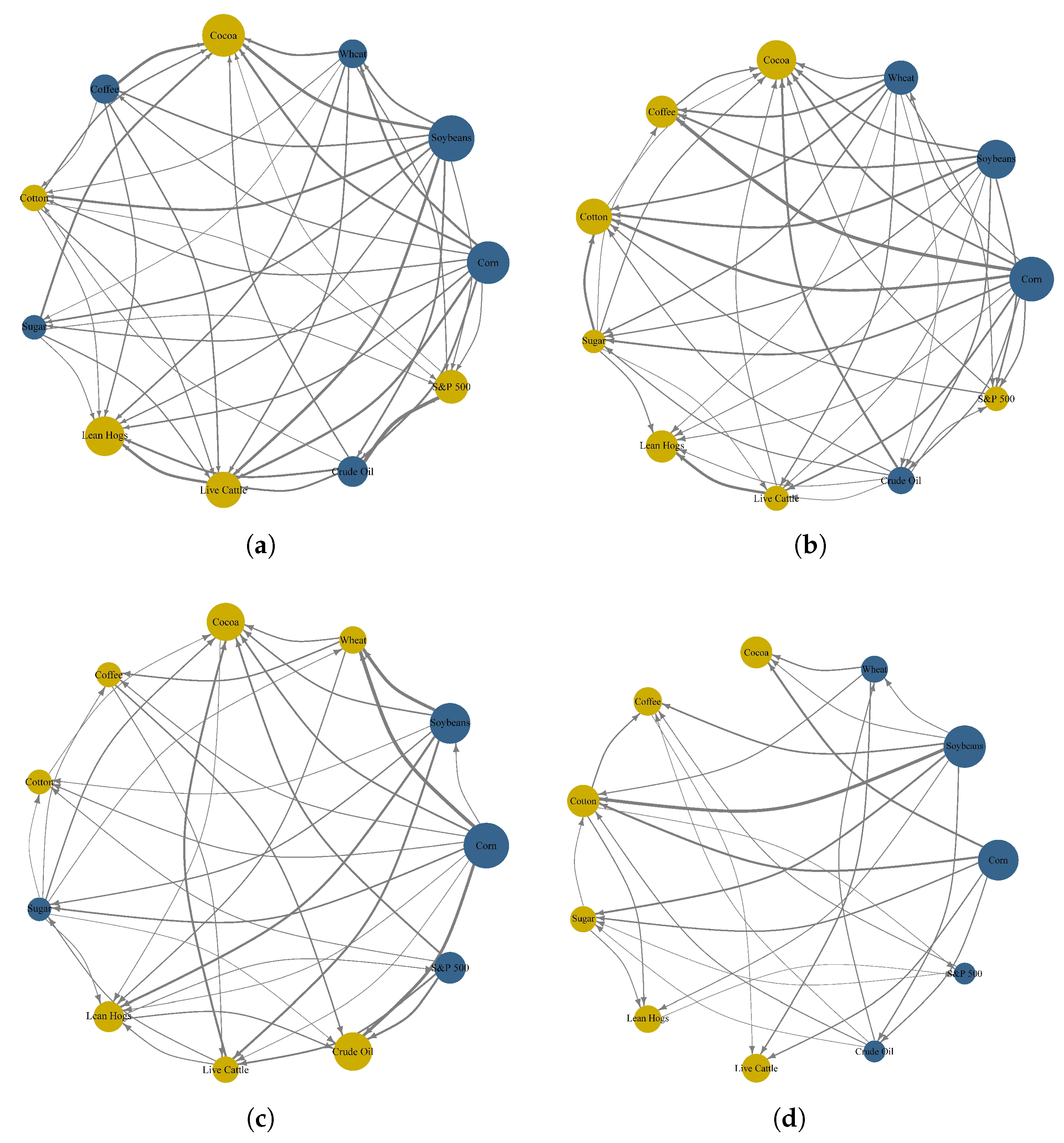
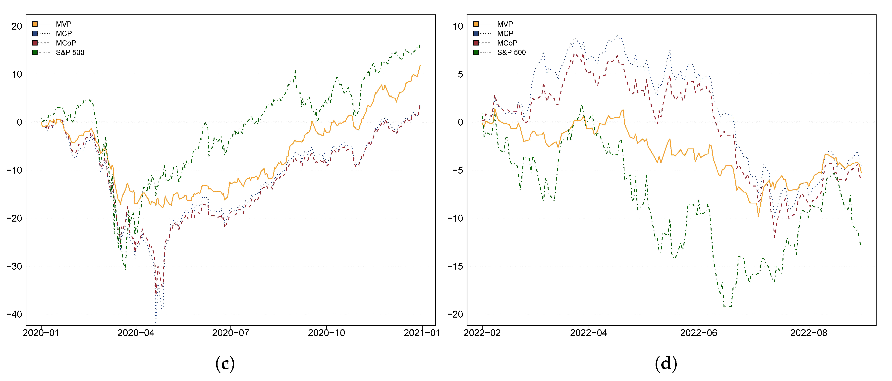
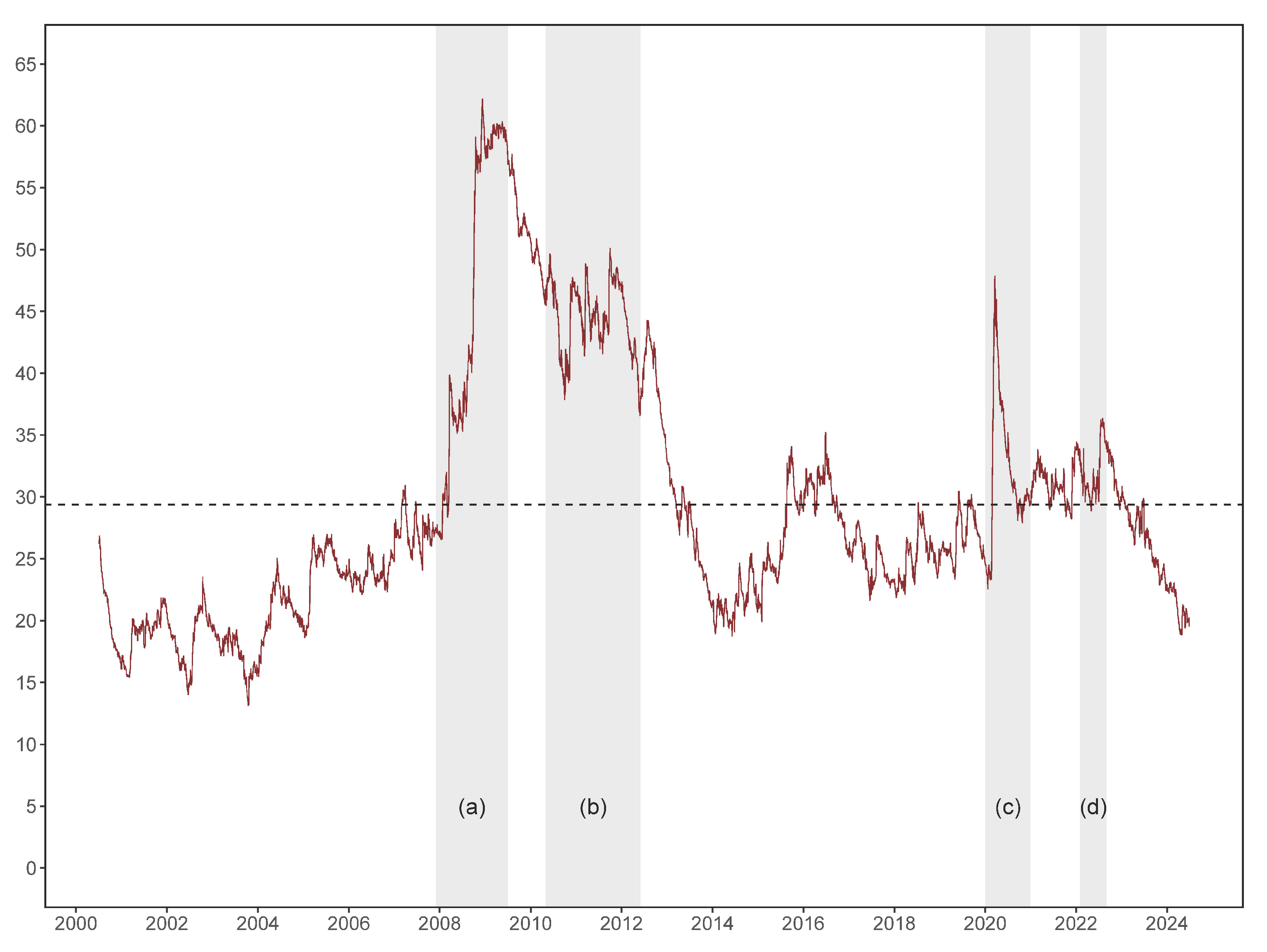
In this section, we perform a robustness check on results, by incorporating additional variables into original model. Specifically, we include two additional soft commodities, cocoa and sugar, as well as one livestock commodity, lean hogs. Figure A1 depicts the dynamic total connectedness index under the new model. The figure shows that the evolution of the TCI do not change. Figure A2 depicts average connectedness network with the inclusion of additional variables. Apart from the switch in the role of sugar, cocoa and lean hogs are always the receiver, and the roles of other original variables remain the same. Figure A3 provides the cumulative return curve for the dynamic portfolio that incorporates the expanded set of commodity indices. We can see they do not change substantially, with only occasional exceptions in the middle phase for global financial crisis. Qualitatively, the inclusion of more agricultural commodities does not alter the connectedness patterns, and the portfolio-related results are highly consistent with our previous findings. Due to space constraints, the remaining results are not reported here but are available upon request.

5. Conclusions

In this study, we conduct a comparative analysis, investigating the dynamic connectedness, portfolio performances, and hedging effectiveness of common agricultural commodities (indices) with the stock market. Specifically, we employ a time-varying parameter vector auto-regression (TVP-VAR) method, applied daily returns of nine agricultural S&P Goldman Sachs Commodity Indices (GSCI), crude oil index, and the S&P 500 index, spanning from July 2000 to June 2024, analyzing the dynamic connectedness among these assets, as well as, the performance of three distinct optimal portfolios during the four turbulent sub-periods.
We confirm the time-varying behaviors of both total and pairwise connectedness among agricultural commodities, crude oil, and the stock market. Over the full sample period, the total connectedness peaked during the 2008 global financial crisis, followed by the European debt crisis and the COVID-19 pandemic, while it remained relatively lower at the onset of the Russia-Ukraine conflict. Additionally, we identify consistent roles for certain assets: corn and soybeans consistently act as transmitters of spillovers, whereas cotton and live cattle are primarily influenced by other markets. In contrast, other commodities, such as wheat, coffee, and crude oil along with the S&P 500, alternate between being receivers and transmitters of shocks across different sub-periods within the network. It is important to note that although the overall system-wide connectedness among commodities and the stock market has gradually declined since the 2008 financial crisis, the bilateral linkage between the agricultural commodities and stock markets has persistently remained above pre-crisis levels.
In portfolio analysis, we use the time varying variance matrix, retrieved from our TVP-VAR framework, construct three portfolios based on criteria of volatility minimization, namely, the minimum variance, the minimum correlation, and the the minimum connectedness portfolio. Our findings suggest that, with exception of the pandemic period, all three dynamic portfolios generate both higher cumulative and risk-adjusted returns than the benchmark (S&P 500 index) during the global events. In terms of three investment strategies, we observe that while the MVP generally achieves lower volatility, the MCP and MCoP strategies outperform in terms of returns in most scenarios. This return superiority is particularly evident in the early phase of each turbulent period. These results confirm that investors can benefit from diversifying their investments into agricultural commodity indices, and dynamic hedging strategies should be adopted rather than static ones. For instance, investors may consider applying the MCP or MCoP strategy to agricultural commodity and stock indices in the early stages of market downturn periods to defense, and then shifting to the traditional MVP strategy in later phases to focus on volatility reduction.
Our results demonstrate how the connectedness between agricultural commodities, crude oil, and the stock market evolves overtime, and evaluate the hedging capabilities of commodities under different strategies for stock market investment amid episodes of market distress. In the context of commodity financialization, these findings offer meaningful insights into the role of agricultural commodities from several perspectives. For regulators and policymakers, preventing and mitigating the risk spillover effects from financial markets to agricultural commodity markets has become more important than ever before. For investors and agribusiness enterprises, adopting a dynamic diversification strategy can enhance returns and reduce exposure to external risks in times of market turbulence. Finally, we acknowledge several limitations in our study. First, our analysis focuses solely on agricultural commodities, leaving the role of other commodities or asset classes unexplored. Second, we consider only the aggregate stock market, without examining sector-specific or characteristic-based equity assets. Future research could extend this work by investigating the connectedness of alternative assets and their hedging potential against equity markets. Additionally, analyzing the dynamic relationships between commodities and sectoral or characteristic-based stock indices may yield valuable insights and flexibility for risk management and portfolio optimization.

Author Contributions

Conceptualization, X.T. and D.L.; methodology, X.T.; software, X.T.; validation, X.T. and D.L.; formal analysis, X.T.; investigation, X.T.; resources, X.T.; data curation, X.T.; writing—original draft preparation, X.T.; writing—review and editing, D.L.; visualization, X.T.; supervision, D.L.; project administration, D.L.; funding acquisition, D.L. All authors have read and agreed to the published version of the manuscript.

Funding

This research received no external funding.

Institutional Review Board Statement

Not applicable.

Informed Consent Statement

Not applicable.

Data Availability Statement

The data that support the findings of this study are available from the Refinitiv Eikon Datastream. Restrictions apply to the availability of these data.

Conflicts of Interest

The authors declare no conflicts of interest.

Appendix A

In this appendix, we provide detailed procedures of the Kalman filter estimation. We first set the prior as Del Negro and Primiceri (2015) for initialization:
vec B 0 N vec B O L S , Σ O L S B , Σ 0 = Σ O L S
Then Kalman filter process can be expressed in:
vec B t z 1 : t 1 N vec B t t 1 , Σ t t 1 B B t t 1 = B t 1 t 1 ϵ t = y t B t t 1 z t 1 Σ t = κ 2 Σ t 1 t 1 + 1 κ 2 ϵ t ϵ t Ξ t = 1 κ 1 1 Σ t 1 t 1 B Σ t t 1 B = Σ t 1 t 1 B + Ξ t Σ t t 1 = z t 1 Σ t t 1 B z t 1 + Σ t
where κ 1 and κ 2 are decay factors, dampening the rate at which the state covariance matrix grows. After that we can update B t , Σ t B , Σ t with the information of time t:
vec B t z 1 : t N vec B t t , Σ t t B K t = Σ t t 1 B z t 1 Σ t t 1 1 B t t = B t t 1 + K t y t B t t 1 z t 1 Σ t t B = I K t Σ t t 1 B ϵ t t = y t B t t z t 1 Σ t t = κ 2 Σ t 1 t 1 + 1 κ 2 ϵ t t ϵ t t
where K t denotes the Kalman gain that explains by how much B t should be adjusted in given state. By multivariate Kalman filter, we can use the estimations of B t further obtain the A i , t .
Table A1. Dynamic multivariate portfolio weights.
Panel A: Global Financial Crisis
VariablesMeanStd. Dev.5%95%HEp-Value
MVPCorn0.020.030.000.070.840.00
Soybeans0.030.030.000.100.820.00
Wheat0.000.000.000.010.880.00
Coffee0.110.050.030.190.740.00
Cotton0.040.020.020.070.820.00
Live Cattle0.700.050.630.810.130.14
Crude Oil0.000.000.000.010.920.00
S&P 5000.090.080.010.240.830.00
MCPCorn0.070.040.010.140.640.00
Soybeans0.040.030.000.090.590.00
Wheat0.120.040.050.170.730.00
Coffee0.120.020.090.140.410.00
Cotton0.130.020.100.170.580.00
Live Cattle0.200.020.160.22−0.950.00
Crude Oil0.080.030.030.130.820.00
S&P 5000.250.030.200.300.610.00
MCoPCorn0.050.040.000.130.640.00
Soybeans0.040.030.000.100.590.00
Wheat0.120.040.050.160.730.00
Coffee0.130.010.100.140.410.00
Cotton0.140.020.120.180.580.00
Live Cattle0.200.020.160.22−0.960.00
Crude Oil0.090.030.050.130.820.00
S&P 5000.230.020.190.250.610.00
Panel B: European Debt Crisis
VariablesMeanStd. Dev.5%95%HEp-Value
MVPCorn0.010.010.000.040.870.00
Soybeans0.180.060.070.260.720.00
Wheat0.000.000.000.000.900.00
Coffee0.030.020.000.060.860.00
Cotton0.050.030.000.100.890.00
Live Cattle0.500.080.310.580.380.00
Crude Oil0.010.020.000.060.850.00
S&P 5000.240.130.110.490.670.00
MCPCorn0.050.030.000.100.740.00
Soybeans0.040.030.000.100.440.00
Wheat0.100.020.070.140.810.00
Coffee0.170.010.150.180.720.00
Cotton0.200.010.180.230.780.00
Live Cattle0.210.030.160.25−0.240.01
Crude Oil0.090.040.050.190.700.00
S&P 5000.130.020.100.160.340.00
MCoPCorn0.050.030.000.090.740.00
Soybeans0.060.020.020.090.440.00
Wheat0.100.020.070.140.810.00
Coffee0.170.010.150.180.720.00
Cotton0.190.010.180.210.780.00
Live Cattle0.190.020.160.23−0.240.01
Crude Oil0.110.030.070.190.700.00
S&P 5000.130.010.110.150.340.00
Panel C: COVID-19 Pandemic
VariablesMeanStd. Dev.5%95%HEp-Value
MVPCorn0.050.080.000.200.630.00
Soybeans0.480.070.370.580.370.00
Wheat0.120.020.080.150.740.00
Coffee0.050.020.020.070.880.00
Cotton0.170.030.130.220.710.00
Live Cattle0.110.050.040.190.780.00
Crude Oil0.000.000.000.000.990.00
S&P 5000.020.030.000.080.870.00
MCPCorn0.010.010.000.03−0.500.00
Soybeans0.060.010.040.08−1.580.00
Wheat0.200.010.170.22−0.070.61
Coffee0.210.020.180.240.520.00
Cotton0.130.020.110.16−0.190.17
Live Cattle0.160.020.120.190.090.46
Crude Oil0.160.020.130.190.950.00
S&P 5000.080.020.050.110.470.00
MCoPCorn0.040.020.010.07−0.390.01
Soybeans0.080.010.060.09−1.380.00
Wheat0.170.010.150.190.010.91
Coffee0.180.010.170.210.560.00
Cotton0.120.010.110.14−0.100.46
Live Cattle0.160.010.140.180.160.17
Crude Oil0.150.010.140.170.950.00
S&P 5000.100.010.090.120.510.00
Panel D: Russia-Ukraine Conflict
VariablesMeanStd. Dev.5%95%HEp-Value
MVPCorn0.160.030.120.200.890.00
Soybeans0.030.020.010.090.860.00
Wheat0.000.000.000.000.960.00
Coffee0.040.010.020.070.910.00
Cotton0.020.010.000.030.920.00
Live Cattle0.590.030.530.630.390.00
Crude Oil0.000.000.000.000.960.00
S&P 5000.170.020.140.190.810.00
MCPCorn0.160.030.130.210.750.00
Soybeans0.000.010.000.030.670.00
Wheat0.100.020.070.130.900.00
Coffee0.140.010.120.170.800.00
Cotton0.080.010.050.100.820.00
Live Cattle0.210.010.190.24−0.410.03
Crude Oil0.060.020.040.090.910.00
S&P 5000.230.010.220.250.560.00
MCoPCorn0.060.020.030.090.710.00
Soybeans0.050.020.030.080.620.00
Wheat0.080.010.060.100.890.00
Coffee0.160.010.160.170.770.00
Cotton0.140.010.120.160.800.00
Live Cattle0.200.010.190.22−0.620.00
Crude Oil0.100.010.080.120.900.00
S&P 5000.200.010.190.210.500.00
Note: The mean weight is the average portion that needs to be invested in each assets, while 5% and 95% represent lower and upper quantiles of optimal daily weights, respectively. HE is the hedging effectiveness which measures the volatility reduction provided by portfolios compared to each asset, and p-value reports the corresponding significance statistics for HE using the Brown and Forsythe (1974) test. Results are derived from the time-varying variance matrix based on one lag structure TVP-VAR (0.99, 0.99) model and a 5-step-ahead (one-week) generalized forecast error variance decomposition.
Figure A1. Dynamic total connectedness. This figure corresponds to Figure 2, with the results derived from the model that incorporates the additional variables of cocoa, sugar, and lean hogs. The shaded area corresponds to four sub-periods: (a) 2008 global financial crisis, (b) European debt crisis, (c) COVID-19 pandemic, and (d) Russia-Ukraine conflict.
Ijfs 13 00143 g0a1
Figure A2. Average connectedness network. This figure corresponds to Figure 3, with the results derived from the model that incorporates the additional variables of cocoa, sugar, and lean hogs: (a) 2008 global financial crisis; (b) European debt crisis; (c) COVID-19 pandemic; (d) Russia-Ukraine conflict.
Ijfs 13 00143 g0a2
Figure A3. Cumulative returns of multivariate portfolios. This figure corresponds to Figure 5, with the results derived from the model that incorporates the additional variables of cocoa, sugar, and lean hogs: (a) 2008 global financial crisis; (b) European debt crisis; (c) COVID-19 pandemic; (d) Russia-Ukraine conflict.
Ijfs 13 00143 g0a3aIjfs 13 00143 g0a3b

Note

1
Diebold and Yilmaz used a generalized variance decompositions scheme according to Koop et al. (1996); Parkinson (1980); Pesaran and Shin (1998).

References

  1. Abakah, E. J. A., Tiwari, A. K., Oliyide, J. A., & Appiah, K. O. (2025). Analyzing the static and dynamic dependence among green investments, carbon markets, financial markets and commodity markets. International Journal of Managerial Finance, 21(1), 286–327. [Google Scholar] [CrossRef]
  2. Ali, S., Bouri, E., Czudaj, R. L., & Shahzad, S. J. H. (2020). Revisiting the valuable roles of commodities for international stock markets. Resources Policy, 66, 101603. [Google Scholar] [CrossRef]
  3. Antonakakis, N., Chatziantoniou, I., & Gabauer, D. (2020). Refined measures of dynamic connectedness based on time-varying parameter vector autoregressions. Journal of Risk and Financial Management, 13(4), 84. [Google Scholar] [CrossRef]
  4. Antonakakis, N., & Gabauer, D. (2017). Refined measures of dynamic connectedness based on TVP-VAR (Tech. Rep.). University Library of Munich. [Google Scholar]
  5. Babar, M., Ahmad, H., & Yousaf, I. (2023). Returns and volatility spillover between agricultural commodities and emerging stock markets: New evidence from COVID-19 and Russian-Ukrainian war. International Journal of Emerging Markets, 19(11), 4049–4072. [Google Scholar] [CrossRef]
  6. Baldi, L., Peri, M., & Vandone, D. (2016). Stock markets’ bubbles burst and volatility spillovers in agricultural commodity markets. Research in International Business and Finance, 38, 277–285. [Google Scholar] [CrossRef]
  7. Banerjee, A. K., Akhtaruzzaman, M., Sensoy, A., & Goodell, J. W. (2024). Volatility spillovers and hedging strategies between impact investing and agricultural commodities. International Review of Financial Analysis, 94, 103237. [Google Scholar] [CrossRef]
  8. Biglova, A., Ortobelli, S., Rachev, S., & Stoyanov, S. (2004). Different approaches to risk estimation in portfolio theory. Journal of Portfolio Management, 31(1), 103. [Google Scholar] [CrossRef]
  9. Broadstock, D. C., Chatziantoniou, I., & Gabauer, D. (2022). Minimum connectedness portfolios and the market for green bonds: Advocating socially responsible investment (SRI) activity. In Applications in energy finance: The energy sector, economic activity, financial markets and the environment (pp. 217–253). Springer. [Google Scholar]
  10. Brown, M. B., & Forsythe, A. B. (1974). Robust tests for the equality of variances. Journal of the American Statistical Association, 69(346), 364–367. [Google Scholar] [CrossRef]
  11. Bunditsakulporn, K. (2022). The relationship between agricultural commodities and stock market in case of Thailand: Safe-haven, hedge, or diversifier?–Cross quantilogram analysis. International Journal of Business & Administrative Studies, 8(3), 127–152. [Google Scholar]
  12. Cagli, E. C., Mandaci, P. E., & Taskin, D. (2023). The volatility connectedness between agricultural commodity and agri businesses: Evidence from time-varying extended joint approach. Finance Research Letters, 52, 103555. [Google Scholar] [CrossRef]
  13. Cagli, E. C. C., Mandaci, P. E., & Taşkın, D. (2023). Environmental, social, and governance (ESG) investing and commodities: Dynamic connectedness and risk management strategies. Sustainability Accounting, Management and Policy Journal, 14(5), 1052–1074. [Google Scholar] [CrossRef]
  14. Campiche, J. L., Bryant, H. L., Richardson, J. W., & Outlaw, J. L. (2007, July 29–August 1). Examining the evolving correspondence between petroleum prices and agricultural commodity prices. The American Agricultural Economics Association Annual Meeting, Portland, OR, USA. [Google Scholar]
  15. Chen, Z., Yan, B., & Kang, H. (2022). Dynamic correlation between crude oil and agricultural futures markets. Review of Development Economics, 1798–1849. [Google Scholar] [CrossRef]
  16. Cheng, I.-H., & Xiong, W. (2014). Financialization of commodity markets. Annual Review of Financial Economics, 6(1), 419–441. [Google Scholar] [CrossRef]
  17. Chien, F., Sadiq, M., Kamran, H. W., Nawaz, M. A., Hussain, M. S., & Raza, M. (2021). Co-movement of energy prices and stock market return: Environmental wavelet nexus of COVID-19 pandemic from the USA, Europe, and China. Environmental Science and Pollution Research, 28(25), 32359–32373. [Google Scholar] [CrossRef] [PubMed]
  18. Christoffersen, P., Errunza, V., Jacobs, K., & Jin, X. (2014). Correlation dynamics and international diversification benefits. International Journal of Forecasting, 30(3), 807–824. [Google Scholar] [CrossRef]
  19. Claessens, S., & Schmukler, S. L. (2007). International financial integration through equity markets: Which firms from which countries go global? Journal of International Money and Finance, 26(5), 788–813. [Google Scholar] [CrossRef]
  20. Del Negro, M., & Primiceri, G. E. (2015). Time varying structural vector autoregressions and monetary policy: A corrigendum. The Review of Economic Studies, 82(4), 1342–1345. [Google Scholar] [CrossRef]
  21. Demirer, M., Diebold, F. X., Liu, L., & Yilmaz, K. (2018). Estimating global bank network connectedness. Journal of Applied Econometrics, 33(1), 1–15. [Google Scholar] [CrossRef]
  22. Dickey, D. A., & Fuller, W. A. (1979). Distribution of the estimators for autoregressive time series with a unit root. Journal of the American Statistical Association, 74(366a), 427–431. [Google Scholar]
  23. Diebold, F. X., & Yilmaz, K. (2009). Measuring financial asset return and volatility spillovers, with application to global equity markets. The Economic Journal, 119(534), 158–171. [Google Scholar] [CrossRef]
  24. Diebold, F. X., & Yilmaz, K. (2012). Better to give than to receive: Predictive directional measurement of volatility spillovers. International Journal of Forecasting, 28(1), 57–66. [Google Scholar] [CrossRef]
  25. Diebold, F. X., & Yilmaz, K. (2014). On the network topology of variance decompositions: Measuring the connectedness of financial firms. Journal of Econometrics, 182(1), 119–134. [Google Scholar] [CrossRef]
  26. Du, L., & He, Y. (2015). Extreme risk spillovers between crude oil and stock markets. Energy Economics, 51, 455–465. [Google Scholar] [CrossRef]
  27. Duménil, G., & Lévy, D. (2004). Capital resurgent: Roots of the neoliberal revolution. Harvard University Press. [Google Scholar]
  28. Ederington, L. H. (1979). The hedging performance of the new futures markets. The Journal of Finance, 34(1), 157–170. [Google Scholar] [CrossRef]
  29. Fisher, T. J., & Gallagher, C. M. (2012). New weighted portmanteau statistics for time series goodness of fit testing. Journal of the American Statistical Association, 107(498), 777–787. [Google Scholar] [CrossRef]
  30. Gabauer, D. (2021). Dynamic measures of asymmetric & pairwise connectedness within an optimal currency area: Evidence from the ERM I system. Journal of Multinational Financial Management, 60, 100680. [Google Scholar] [CrossRef]
  31. Garcia-Jorcano, L., & Sanchis-Marco, L. (2022). Spillover effects between commodity and stock markets: A SDSES approach. Resources Policy, 79, 102926. [Google Scholar] [CrossRef]
  32. Gatfaoui, H. (2016). Linking the gas and oil markets with the stock market: Investigating the US relationship. Energy Economics, 53, 5–16. [Google Scholar] [CrossRef]
  33. Giunta, N., Orlando, G., Carleo, A., & Ricci, J. M. (2024). Exploring entropy-based portfolio strategies: Empirical analysis and cryptocurrency impact. Risks, 12(5), 78. [Google Scholar] [CrossRef]
  34. Goodwin, T. H. (1998). The information ratio. Financial Analysts Journal, 54(4), 34–43. [Google Scholar] [CrossRef]
  35. Hadad, E., Malhotra, D., & Vasileiou, E. (2024). Risk spillovers and optimal hedging in commodity ETFs: A TVP-VAR Approach. Finance Research Letters, 70, 106372. [Google Scholar] [CrossRef]
  36. Han, S. (2025). Evaluating the hedging potential of energy, metals, and agricultural commodities for US stocks post-COVID-19. The North American Journal of Economics and Finance, 77, 102380. [Google Scholar] [CrossRef]
  37. Hernandez, J. A., Kang, S. H., & Yoon, S.-M. (2021). Spillovers and portfolio optimization of agricultural commodity and global equity markets. Applied Economics, 53(12), 1326–1341. [Google Scholar] [CrossRef]
  38. Hung, N. T. (2021). Oil prices and agricultural commodity markets: Evidence from pre and during COVID-19 outbreak. Resources Policy, 73, 102236. [Google Scholar] [CrossRef] [PubMed]
  39. Jarque, C. M., & Bera, A. K. (1980). Efficient tests for normality, homoscedasticity and serial independence of regression residuals. Economics Letters, 6(3), 255–259. [Google Scholar] [CrossRef]
  40. Jebabli, I., Kouaissah, N., & Arouri, M. (2022). Volatility spillovers between stock and energy markets during crises: A comparative assessment between the 2008 global financial crisis and the COVID-19 pandemic crisis. Finance Research Letters, 46, 102363. [Google Scholar] [CrossRef]
  41. Kang, J.-S., Hu, J.-L., Chen, C.-W., & Hu, J.-L. (2013). Linkage between international food commodity prices and the Chinese stock markets. International Journal of Economics and Finance, 5(10), 147. [Google Scholar] [CrossRef]
  42. Kang, S. H., McIver, R., & Yoon, S.-M. (2017). Dynamic spillover effects among crude oil, precious metal, and agricultural commodity futures markets. Energy Economics, 62, 19–32. [Google Scholar] [CrossRef]
  43. Kang, W., Tang, K., & Wang, N. (2023). Financialization of commodity markets ten years later. Journal of Commodity Markets, 30, 100313. [Google Scholar] [CrossRef]
  44. Koop, G., & Korobilis, D. (2014). A new index of financial conditions. European Economic Review, 71, 101–116. [Google Scholar] [CrossRef]
  45. Koop, G., Pesaran, M. H., & Potter, S. M. (1996). Impulse response analysis in nonlinear multivariate models. Journal of Econometrics, 74(1), 119–147. [Google Scholar] [CrossRef]
  46. Korobilis, D., & Yilmaz, K. (2018). Measuring dynamic connectedness with large bayesian var models [Working Paper]. Available online: https://ssrn.com/abstract=3099725 (accessed on 30 August 2023).
  47. Li, B., Haneklaus, N., & Rahman, M. M. (2024). Dynamic connectedness and hedging opportunities of the commodity and stock markets in China: Evidence from the TVP-VAR and cDCC-FIAPARCH. Financial Innovation, 10(1), 52. [Google Scholar] [CrossRef]
  48. Liu, Z., Tseng, H.-K., Wu, J. S., & Ding, Z. (2020). Implied volatility relationships between crude oil and the US stock markets: Dynamic correlation and spillover effects. Resources Policy, 66, 101637. [Google Scholar] [CrossRef]
  49. Ljung, G. M., & Box, G. E. (1978). On a measure of lack of fit in time series models. Biometrika, 65(2), 297–303. [Google Scholar] [CrossRef]
  50. Markovitz, H. (1959). Portfolio selection: Efficient diversification of investments. John Wiley. [Google Scholar]
  51. Martin, P. G., & McCann, B. B. (1989). The investor’s guide to fidelity funds: Winning strategies for mutual fund investors. John Wiley & Sons, Inc. [Google Scholar]
  52. Mujtaba, G., Siddique, A., Naifar, N., & Shahzad, S. J. H. (2024). Hedge and safe haven role of commodities for the US and Chinese equity markets. International Journal of Finance & Economics, 29(2), 2381–2414. [Google Scholar]
  53. Parkinson, M. (1980). The extreme value method for estimating the variance of the rate of return. Journal of Business, 53(1), 61–65. [Google Scholar] [CrossRef]
  54. Pesaran, H. H., & Shin, Y. (1998). Generalized impulse response analysis in linear multivariate models. Economics Letters, 58(1), 17–29. [Google Scholar] [CrossRef]
  55. Pinho, C., & Maldonado, I. (2022). Commodity and equity markets: Volatility and return spillovers. Commodities, 1(1), 18–33. [Google Scholar] [CrossRef]
  56. Primiceri, G. E. (2005). Time varying structural vector autoregressions and monetary policy. The Review of Economic Studies, 72(3), 821–852. [Google Scholar] [CrossRef]
  57. Reboredo, J. C., Ugolini, A., & Hernandez, J. A. (2021). Dynamic spillovers and network structure among commodity, currency, and stock markets. Resources Policy, 74, 102266. [Google Scholar] [CrossRef]
  58. Roll, R. (1992). A mean/variance analysis of tracking error. Journal of Portfolio Management, 18(4), 13–22. [Google Scholar] [CrossRef]
  59. Rubbaniy, G., Khalid, A. A., Syriopoulos, K., & Samitas, A. (2022). Safe-haven properties of soft commodities during times of COVID-19. Journal of Commodity Markets, 27, 100223. [Google Scholar] [CrossRef]
  60. Rubbaniy, G., Maghyereh, A., Cheffi, W., & Khalid, A. A. (2024). Dynamic connectedness, portfolio performance, and hedging effectiveness of the hydrogen economy, renewable energy, equity, and commodity markets: Insights from the COVID-19 pandemic and the Russia-Ukraine war. Journal of Cleaner Production, 452, 142217. [Google Scholar] [CrossRef]
  61. Sevillano, M. C., Jareño, F., López, R., & Esparcia, C. (2024). Connectedness between oil price shocks and US sector returns: Evidence from TVP-VAR and wavelet decomposition. Energy Economics, 131, 107398. [Google Scholar] [CrossRef]
  62. Sharpe, W. F. (1966). Mutual fund performance. The Journal of Business, 39(1), 119–138. [Google Scholar] [CrossRef]
  63. Sortino, F. A., & Van Der Meer, R. (1991). Downside risk. Journal of Portfolio Management, 17(4), 27. [Google Scholar] [CrossRef]
  64. Tobler, A., Haase, M., & Sigg, P. (2017). Integrating Sustainability into Commodity Investing. In Handbook on sustainable investments: Background information and practical examples for institutional asset owners (pp. 129–133). CFA Institute Research Foundation. [Google Scholar]
  65. Wen, X., Wei, Y., & Huang, D. (2012). Measuring contagion between energy market and stock market during financial crisis: A copula approach. Energy Economics, 34(5), 1435–1446. [Google Scholar] [CrossRef]
  66. Wu, F., Guan, Z., & Myers, R. J. (2011). Volatility spillover effects and cross hedging in corn and crude oil futures. Journal of Futures Markets, 31(11), 1052–1075. [Google Scholar] [CrossRef]
  67. Xu, W., Ma, F., Chen, W., & Zhang, B. (2019). Asymmetric volatility spillovers between oil and stock markets: Evidence from China and the United States. Energy Economics, 80, 310–320. [Google Scholar] [CrossRef]
  68. Zhang, H., Chen, J., & Shao, L. (2021). Dynamic spillovers between energy and stock markets and their implications in the context of COVID-19. International Review of Financial Analysis, 77, 101828. [Google Scholar] [CrossRef]
  69. Zhu, B., Lin, R., Deng, Y., Chen, P., & Chevallier, J. (2021). Intersectoral systemic risk spillovers between energy and agriculture under the financial and COVID-19 crises. Economic Modelling, 105, 105651. [Google Scholar] [CrossRef]
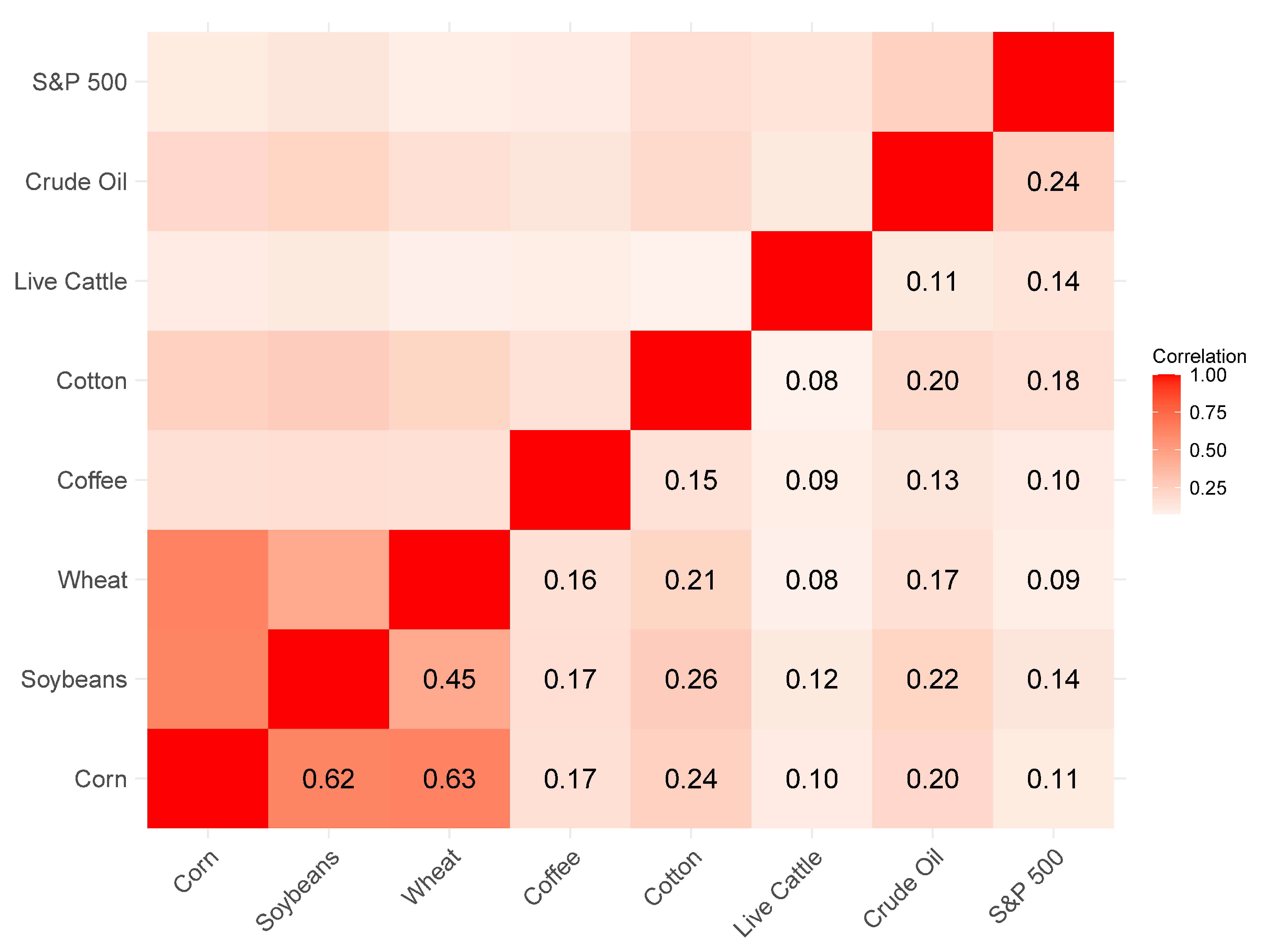
Figure 1. Pearson correlation coefficient matrix. This figure displays the Pearson correlation coefficient matrix of index returns over the full sample.
Ijfs 13 00143 g001
Figure 2. Dynamic total connectedness. This figure displays the dynamic total return connectedness for the full sample. The shaded area corresponds to four sub-periods: (a) 2008 global financial crisis, (b) European debt crisis, (c) COVID-19 pandemic, and (d) Russia-Ukraine conflict. Note: Results are obtained from one lag structure TVP-VAR ( 0.99 , 0.99 ) model and a 5-step-ahead (one-week) generalized forecast error variance decomposition.
Ijfs 13 00143 g002
Figure 3. Average connectedness network. This figure illustrates the average net pairwise directional connectedness among all commodities and the S&P 500 during the different sub-sample periods: (a) 2008 global financial crisis; (b) European debt crisis; (c) COVID-19 pandemic; (d) Russia-Ukraine conflict. Note: The color and size of the nodes indicate whether the commodity or the stock market acts as a transmitter (blue) or receiver (yellow) and average weighted connectedness, while the direction and thickness of the arrows between the nodes represent the magnitude of the connectedness. Results are obtained from one lag structure TVP-VAR ( 0.99 , 0.99 ) model and a 5-step-ahead (one-week) generalized forecast error variance decomposition.
Ijfs 13 00143 g003
Figure 4. Individual commodity pairwise connectedness index with S&P 500. This figure illustrates the dynamic bilateral connectedness score between sampled commodities and S&P 500 index over the full sample period. Note: The index score is standardized, ranging from 0 to 100. Results are derived from one lag structure TVP-VAR ( 0.99 , 0.99 ) model and a 5-step-ahead (one-week) generalized forecast error variance decomposition.
Ijfs 13 00143 g004
Figure 5. Cumulative returns of multivariate portfolios. This figure illustrates the cumulative returns (%) of minimum variance portfolio (MVP), minimum correlation portfolio (MCP), and minimum connectedness portfolio (MCoP) across four sub-sample periods: (a) 2008 global financial crisis; (b) European debt crisis; (c) COVID-19 pandemic; (d) Russia-Ukraine conflict. Note: Results are obtained from the time-varying variance matrix based on one lag structure TVP-VAR ( 0.99 , 0.99 ) model and a 5-step-ahead (one-week) generalized forecast error variance decomposition. We use the unhedged S&P 500 index cumulative returns as the benchmark.
Ijfs 13 00143 g005
Figure 6. Dynamic weights of multivariate portfolios. This figure displays the daily assets allocation weights for minimum variance portfolio (MVP), minimum correlation portfolio (MCP), and minimum connectedness portfolio (MCoP) for the full sample. Note: Results are derived from time-varying variance matrix based on one lag structure TVP-VAR ( 0.99 , 0.99 ) model and a 5-step-ahead (one-week) generalized forecast error variance decomposition.
Ijfs 13 00143 g006
Table 1. Descriptive statistics.
VariablesMean (%)Max. (%)Min. (%)Std. Dev.SkewnessKurtosisJarque-BeraL-B Q(20)L-B Q2(20)ADF
Corn0.018.66−8.121.65−0.012.461574.44 ***30.97 ***1092.80 ***−17.25 ***
Soybeans0.016.43−7.341.44−0.222.521707.56 ***16.05 *1246.35 ***−16.89 ***
Wheat0.018.79−10.021.910.121.961021.30 ***9.021187.46 ***−19.30 ***
Coffee0.0216.39−13.382.040.173.012398.67 ***22.27 ***1051.19 ***−19.50 ***
Cotton0.008.53−7.131.68−0.061.41522.15 ***31.45 ***1307.32 ***−17.71 ***
Live Cattle0.025.45−6.360.99−0.162.461604.98 ***75.79 ***2690.00 ***−16.86 ***
Crude Oil0.0243.79−56.862.59−1.4461.15977,190.43 ***107.21 ***1615.66 ***−17.93 ***
S&P 5000.0210.96−12.771.20−0.3911.2933,389.67 ***98.94 ***5765.25 ***−18.58 ***
Note: The table reports the descriptive statistics for daily logarithmic returns (100 * (ln r i , t − ln r i , t 1 )) of the S&P 500 and commodity indices for full sample. Jarque-Bera (Jarque & Bera, 1980) is the test for Gaussian distribution. L-B Q(20) is the Ljung-Box Q test (Ljung & Box, 1978) with lag length of 20. L - B Q 2 ( 20 ) is the new weighted portmanteau statistics (Fisher & Gallagher, 2012) with lag length of 20. ADF is the augmented Dickey-Fuller test (Dickey & Fuller, 1979) for series stationary. *, **, and *** indicate significance at the 10%, 5% and 1% level, respectively.
Table 2. Return connectedness table.
Panel A: Full Sample
VariablesCornSoybeansWheatCoffeeCottonLive CattleCrude OilS&P 500From
Corn50.8719.3920.201.883.081.182.530.8849.13
Soybeans21.0455.4010.842.443.871.343.431.6344.60
Wheat22.5411.1757.342.072.451.142.380.9142.66
Coffee3.003.522.9281.112.651.562.952.2918.89
Cotton4.265.003.162.5876.421.363.763.4523.58
Live Cattle1.892.161.681.551.5986.761.952.4113.24
Crude Oil3.284.302.572.573.471.6975.896.2424.11
S&P 5001.322.061.282.143.442.036.6981.0418.96
TO57.3247.6042.6515.2320.5610.3123.7017.80cTCI/TCI
NET8.193.01−0.01−3.65−3.02−2.94−0.42−1.1633.60/29.40
Panel B: Global Financial Crisis
VariablesCornSoybeansWheatCoffeeCottonLive CattleCrude OilS&P 500From
Corn36.2018.6414.447.828.053.788.742.3363.80
Soybeans18.5236.2411.778.248.854.129.992.2763.76
Wheat16.6713.3741.467.637.073.428.242.1458.54
Coffee9.9310.688.3645.789.124.157.614.3754.22
Cotton9.6311.258.129.2646.803.997.263.6953.20
Live Cattle6.176.674.965.415.0759.816.745.1540.19
Crude Oil10.8511.788.607.216.434.9544.455.7355.55
S&P 5003.143.173.184.404.154.718.7768.4831.52
TO74.9275.5659.4249.9748.7529.1257.3525.69cTCI/TCI
NET11.1211.810.88−4.24−4.45−11.071.80−5.8460.11/52.60
Panel C: European Debt Crisis
VariablesCornSoybeansWheatCoffeeCottonLive CattleCrude OilS&P 500From
Corn43.7716.9222.083.563.953.583.962.1956.23
Soybeans17.3545.1714.783.904.832.636.384.9554.83
Wheat22.9214.9245.922.943.533.023.763.0054.08
Coffee6.856.035.0464.392.814.095.295.5035.61
Cotton6.437.105.412.6968.790.864.374.3431.21
Live Cattle5.823.944.694.291.2871.894.054.0428.11
Crude Oil5.237.834.524.943.463.1355.7915.1044.21
S&P 5003.396.413.974.993.273.5015.8758.6041.40
TO67.9963.1560.4927.3023.1320.8143.6839.12cTCI/TCI
NET11.768.326.41−8.31−8.07−7.30−0.53−2.2849.38/43.21
Panel D: COVID-19 Pandemic
VariablesCornSoybeansWheatCoffeeCottonLive CattleCrude OilS&P 500From
Corn51.9120.597.323.535.691.905.014.0548.09
Soybeans21.0754.138.515.063.393.491.522.8445.87
Wheat10.2311.0773.851.130.481.220.841.2026.15
Coffee3.995.122.4583.900.731.901.240.6616.10
Cotton6.524.030.530.4465.082.815.6214.9734.92
Live Cattle2.455.491.742.873.2476.321.586.3123.68
Crude Oil7.541.941.092.746.181.4971.087.9528.92
S&P 5004.363.280.970.6614.234.555.9865.9934.01
TO56.1651.5122.6216.4333.9317.3521.7837.97cTCI/TCI
NET8.075.64−3.530.33−0.99−6.33−7.143.9536.82/32.22
Panel E: Russia-Ukraine Conflict
VariablesCornSoybeansWheatCoffeeCottonLive CattleCrude OilS&P 500From
Corn44.1219.9521.040.504.240.678.481.0255.88
Soybeans20.7947.399.873.975.050.6610.921.3552.61
Wheat22.0210.9945.951.643.140.1515.150.9754.05
Coffee0.976.611.4976.766.421.364.451.9523.24
Cotton7.179.484.544.0367.740.545.141.3632.26
Live Cattle2.390.622.082.040.4890.970.540.889.03
Crude Oil10.4912.7813.453.343.850.7254.680.6845.32
S&P 5001.450.651.780.671.880.900.5492.137.87
TO65.2861.0854.2416.1925.064.9945.228.21cTCI/TCI
NET9.408.470.18−7.05−7.21−4.05−0.100.3540.04/35.03
Note: We select one lag for our VAR structure and use a 5-step-ahead (one-week) generalized forecast error variance decomposition. The decay factors in the Kalman filter algorithm for our TVP-VAR is (0.99, 0.99). The diagonal elements of each panel estimate each asset’s own variance share, while the off-diagonal elements represent the asset’s contribution to spillovers ‘from’ or ‘to’ others.
Table 3. Risk-adjusted portfolio performance.
Panel A: Global Financial Crisis
MeasuresPhasesStd. Dev.Sortino RatioUlcer IndexRachev RatioTracking ErrorInformation Ratio
early0.73700.08480.03131.01521.29260.0671
MVP middle1.0735−0.07530.18290.80492.36430.0343
late0.98520.02730.04600.89151.89900.0057
early1.01410.03890.05560.79161.29950.0569
MCP middle1.6422−0.07300.29010.76891.89320.0263
late1.46480.04910.04860.83391.43600.0307
early1.02500.04410.05450.77831.32250.0593
MCoP middle1.6439−0.07370.29260.77041.93650.0253
late1.46660.05070.04820.83251.45600.0315
early1.3097−0.04720.09990.9428
S&P 500 middle2.6970−0.07150.35790.8847
late2.17190.00560.10740.9584
Panel B: European Debt Crisis
MeasuresPhasesStd. Dev.Sortino RatioUlcer IndexRachev RatioTracking ErrorInformation Ratio
early0.72570.19450.03580.96541.01380.0766
MVP middle0.72070.00000.06680.90811.0016−0.0141
late0.6325−0.06640.03740.99790.9912−0.0722
early1.05670.27640.03551.14871.11150.1494
MCP middle0.9992−0.06110.19160.81451.1134−0.0546
late0.7885−0.12500.05570.81700.9623−0.1226
early1.06130.26680.03571.14131.10670.1452
MCoP middle0.9995−0.05890.18330.81441.1021−0.0537
late0.8060−0.12290.05500.81040.9621−0.1232
early1.25700.01910.08171.0214
S&P 500 middle1.25480.01520.07840.8738
late1.08350.05660.03591.0323
Panel C: COVID-19 Pandemic
MeasuresPhasesStd. Dev.Sortino RatioUlcer IndexRachev RatioTracking ErrorInformation Ratio
early0.8732−0.28520.09900.53193.0635−0.0177
MVP middle0.69680.42890.01101.26871.27210.0221
late0.71660.51220.01211.20301.12130.0700
early1.7434−0.26100.15950.71602.8256−0.0722
MCP middle1.48750.16270.02951.03571.47800.0198
late0.84850.30390.01611.13621.08510.0240
early1.7368−0.25800.15710.70082.7757−0.0717
MCoP middle1.39720.17120.02691.02951.39230.0211
late0.82560.34330.01491.16241.03970.0387
early3.4539−0.06650.16730.8705
S&P 500 middle1.24260.15980.03520.7982
late1.04270.19020.02300.9701
Panel D: Russia-Ukraine Conflict
MeasuresPhasesStd. Dev.Sortino RatioUlcer IndexRachev RatioTracking ErrorInformation Ratio
early0.5507−0.11340.03060.90701.3748−0.0262
MVP middle0.7074−0.04450.05770.73641.37140.0826
late0.59520.28040.00551.02491.13890.0271
early0.88570.27550.01601.12551.71870.0939
MCP middle1.0476−0.10510.09330.74961.46370.0355
late1.13430.03400.02930.79001.3838−0.0359
early0.94120.16310.01960.97161.73130.0643
MCoP middle1.1287−0.09950.09290.79381.50260.0338
late1.18930.02980.02970.79161.4087−0.0369
early1.3997−0.01060.04840.9149
S&P 500 middle1.5779−0.11170.12800.7274
late1.22200.09880.02551.1389
Note: The early phase is defined as the first 30 % of return data within each sub-sample period, the middle phase corresponds to the central 40 % , and the late phase captures the final 30 % return performance. Results are derived from the time-varying variance covariance matrix based on one lag structure TVP-VAR ( 0.99 , 0.99 ) model and a 5-step-ahead (one-week) generalized forecast error variance decomposition. Since the tracking error and information ratio are calculated relative to the S&P 500 benchmark, they are not applicable to the S&P 500 itself.
Disclaimer/Publisher’s Note: The statements, opinions and data contained in all publications are solely those of the individual author(s) and contributor(s) and not of MDPI and/or the editor(s). MDPI and/or the editor(s) disclaim responsibility for any injury to people or property resulting from any ideas, methods, instructions or products referred to in the content.