Article

Dynamics of Green and Conventional Bonds: Hedging Effectiveness and Sustainability Implication

Probability and Statistics Laboratory (LR), Faculty of Business and Economic Sciences, University of Sfax, Sfax 3029, Tunisia
Int. J. Financial Stud. 2025, 13(2), 106; https://doi.org/10.3390/ijfs13020106
Submission received: 5 April 2025 / Revised: 8 May 2025 / Accepted: 27 May 2025 / Published: 6 June 2025
(This article belongs to the Special Issue Investment and Sustainable Finance)

Abstract

This research examines the challenges of issuing green bonds due to a lack of established benchmarks. We compare regional differences between the U.S. and the E.U., hypothesizing that issuers of green bonds stand to benefit from comparing them to conventional (black) bonds. As most investors prioritize net positive returns as opposed to intangible sustainability metrics, the existence of a “green premium”, defined as the opportunity to price green bonds differently, remains to be proven. To this end, we employ a time-varying parameter vector autoregression (TVP-VAR), first deriving dynamic variance–covariance matrices and then conducting variance decomposition analysis to gauge connectedness and spillover effects of various bond benchmarks. Implementing multivariate portfolio construction strategies, we investigate the hedging capabilities of green and black bonds. Our findings show that both green and black bonds contribute to portfolio diversification as a risk management strategy. The paper highlights the role played by green bonds in promoting financial stability.

1. Introduction

Increasing awareness of the impacts of climate change has, in recent years, shifted the global financial sector towards sustainability. Governments and private investors, realizing the implications of climate change for economies, are demanding more environmentally friendly investment options. This shift in priorities has led to the rise of “green bonds”, inventive financial instruments specifically designed to fund projects that promise positive environmental impact.
The issuance of these green bonds has attracted a diverse pool of investors, dramatically expanding to encompass a wide range of sectors. Particularly, institutional investors have significantly increased the proportion of green bonds in their portfolios, their motivation now being more than just the positive net returns (Guo & Zhou, 2021). Regulatory frameworks, having caught on, are actively championing for green finance through initiatives such as the European Union’s Green Deal and the United Nations’ Sustainable Development Goals.
The main objective of this research is to evaluate how green bonds contribute to improving portfolio stability and hedging effectiveness in U.S. and E.U. financial markets. More specifically, the paper aims to examine the dynamic connectedness and shock transmission between green and black bonds, compare the hedging effectiveness of green versus conventional bonds using dynamic portfolio strategies, and assess whether regional differences (U.S. vs. E.U.) influence the performance and role of green bonds. Based on these objectives, we pose the following hypotheses:
(1) Green bonds contribute significantly to risk reduction and portfolio diversification;
(2) Green bonds exhibit different connectedness and shock transmission dynamics compared to conventional bonds;
(3) Regional variations (U.S. vs. E.U.) impact the hedging performance of green bonds.
Several prior studies explored the role of green bonds in investment strategies and their implications for financial markets. For instance, Abuzayed and Al-Fayoumi (2023) highlighted the safe-haven potential of green bonds during the COVID-19 crisis, Guo and Zhou (2021) demonstrated their changing hedging behavior before and after the pandemic, and Ejaz et al. (2022) underscored their increasing integration with global financial markets. However, the existing literature often focuses on the standalone performance of green bonds without a comprehensive exploration of their connectedness with traditional bonds and the broader financial system, particularly using dynamic frameworks like the TCI. Moreover, green bonds remain at a relatively early stage of development, often lacking robust benchmarks. Thus, we hypothesize two strategic approaches for issuance: (i) comparing green bonds to conventional (black) bonds using established benchmarks and (ii) analyzing regional differences between U.S. and E.U. markets to inform issuance and investment strategies. Our hypotheses are challenged by the ongoing debate over the existence of a ‘green premium’, the idea that green bonds can be priced differently than black bonds with similar financial specifications. While socially responsible investing (SRI) suggests that sustainability influences investment decisions, it is likely that most investors prioritize financial returns. Therefore, this paper deliberately adopts a market-driven perspective, focusing on how green bonds behave relative to conventional ones across different economic regions, rather than on behavioral or preference-driven aspects.
For hypothesis formulation, we first estimate a time-varying parameter vector autoregression (TVP-VAR) from which we derive dynamic variance–covariance matrices, following the study by Antonakakis et al. (2020). These matrices form the basis for the subsequent portfolio formation. Afterward, we apply variance decomposition analysis, as used by Diebold and Yilmaz (2009, 2012), to examine the connectedness and spillover effects among the various bond index benchmarks. Third, we implement four multivariate portfolio construction strategies: (i) time-varying minimum variance, (ii) minimum correlation, (iii) minimum connectedness, and (iv) risk parity portfolios. Each of these methods leverages the estimated dynamic variance–covariance matrices. Finally, by evaluating their hedging capabilities, we investigate the significance of green bonds in a well-balanced fixed-income portfolio.
This paper offers a three-fold incremental contribution. First, it explores the TCI and shock transmission dynamics among U.S. and E.U. bond assets, including traditional and green bonds, from June 2021 to May 2024. Second, it examines the effectiveness of green bonds in multivariate portfolio risk management and hedging strategies, particularly during periods of economic stress. Lastly, it provides implications for investors regarding the role of green bonds in enhancing portfolio resilience, particularly in alignment with environmental, social, and governance (ESG) criteria and sustainability objectives.
Our findings show that green and black bonds from the U.S. and E.U. play a crucial role in portfolio diversification and risk management, particularly during periods of market stress, such as the post-COVID-19 recovery period and the Russia–Ukraine conflict. Across the four portfolio strategies—Minimum Variance, Minimum Connectedness, Minimum Correlation, and in the context of risk parity strategies, EU green bonds consistently showed higher hedging effectiveness, highlighting their significant role in reducing portfolio risk. These findings underscore the value of green bonds as essential components in fixed-income portfolios, contributing to both financial stability and sustainability objectives.
The rest of this paper is organized as follows: Section 2 reviews the currently available literature on green bonds; Section 3 details the data used in our analysis; Section 4 outlines the economic framework supporting this study Section 5 presents the findings; Section 6 concludes the discussion.

2. Literature Review

A common theme in the literature on green bonds is their ability to act as effective hedging instruments during periods of financial distress and heightened volatility. Their growing appeal lies in their dual function: reducing risk in fixed-income portfolios while advancing sustainability goals. This section provides a structured overview of the growing body of research on green bonds, focusing on their fundamental principles, pricing behavior, market dynamics, and financial implications. It highlights both theoretical and empirical findings that inform their role in portfolio diversification, risk management, and sustainable finance. The review is organized into four thematic sub-sections to clarify key aspects shaping green bond performance and investor decision-making.

2.1. The Essence and Principles of Issuing Green Bonds

The core principle behind green bonds lies in their targeted use of proceeds for environmentally sustainable projects, which distinguishes them from conventional bonds. Khan et al. (2019) explore the evolution of green ideology within Asian emerging economies, focusing on the intersection of environmental policy and sustainable development. Their research highlights how these economies are transitioning towards sustainability by integrating green policies into their development frameworks.

2.2. The Greenium: Price Difference Between Conventional and Green Bonds

Arat et al. (2023) showed that in the face of drastic market volatility, green bonds tend to outperform conventional bonds. They compared the greenium (the yield difference between green and conventional bonds) before and after the COVID-19 pandemic, revealing a widening gap from 1.6 to 3.5 basis points. This suggests that green bonds are perceived as more resilient and desirable, even at slightly lower yields. Zerbib (2019) also explores the greenium and shows that while statistically significant, the price advantage of green bonds varies depending on issuer types and market conditions, reinforcing the complexity of green bond pricing.

2.3. Identification of Pricing Factors and Market Dynamics of Green Bonds

Peng et al. (2023) highlighted the positive spillover effects from green bonds to conventional bonds, which further enhance portfolio resilience. Zhao and Park (2024) added a bidirectional component in their investigation, showing green bonds to transmit short-term risk but absorb long-term shocks from conventional bonds. These findings underline the complexity and dynamic nature of green bond market behavior.
Mensi et al. (2024) found that market conditions greatly affect the connectedness between green and conventional bonds—intensifying during volatility. Wang et al. (2024) similarly revealed that green bonds absorb and transmit shocks depending on market stability. Reboredo and Ugolini (2020) showed spillovers from fixed-income and currency markets to green bonds, but little reverse effect—reinforcing their role as risk absorbers. Huynh (2022) used entropy and copulas to identify contagion risks between green and AAA government bonds, reinforcing systemic links.
Flammer (2021) finds that green bond issuance improves firms’ environmental performance and investor perception, suggesting that issuer credibility and transparency can be key pricing factors. Karpf and Mandel (2018) analyze structural differences in green bond pricing and highlight the influence of liquidity, credit quality, and issuer reputation on yield spreads.

2.4. Benefits and Risks of Green Bond Issuance for Issuers and Investors
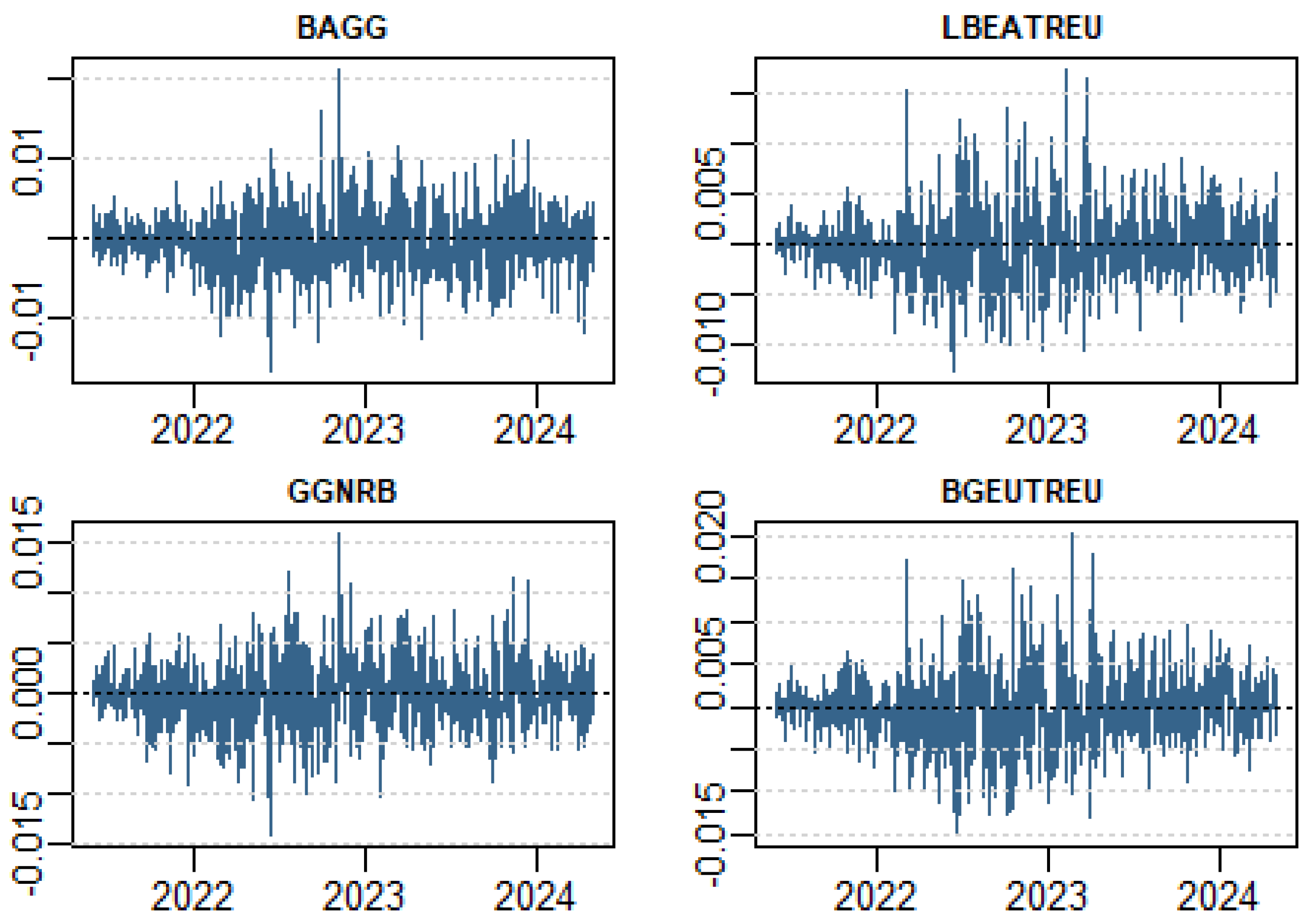
Broadstock et al. (2022) investigated the value-enhancing role of green bonds in global fixed-income portfolios, finding proportions of 40–80% in optimized portfolios. Tsoukala and Tsiotas (2021) evidenced strong volatility spillovers between green and conventional bonds during crisis periods, highlighting the importance of managing interconnected risks.
Khamis and Aassouli (2023) reviewed studies on green bonds’ roles as diversifiers, hedges, and safe havens, though they found limited benefits when held alongside conventional bonds. Naeem et al. (2021) found green bonds to be more efficient than traditional bonds during COVID-19, supporting their usefulness in crisis-driven portfolios. Man et al. (2023), Wang et al. (2024), and Contractor et al. (2023) confirmed green bonds’ superior hedging potential during distress while Xu et al. (2024) and Yousfi and Bouzgarrou (2024) validated the use of minimum connectedness portfolios for higher risk-adjusted returns. Imran and Ahad (2023) further showed their safe-haven characteristics during major crises like the COVID-19 pandemic. Mohammed et al. (2024) found green bonds to be negatively correlated with financial risk from geopolitical events (e.g., Ukraine war, U.S. policy tightening). Lichtenberger et al. (2022) and Han and Li (2022) highlighted higher Sharpe ratios and lower volatility, reinforcing the financial attractiveness of green bonds beyond ESG motivations. Finally, Ejaz et al. (2022) and Abuzayed and Al-Fayoumi (2023) emphasized the benefits of optimized portfolio weighting with green bonds for effective risk mitigation. Bachelet et al. (2019) further investigated the performance of green bonds and showed that while they are not always cheaper to issue, they offer reputational benefits and contribute to long-term investor trust.

3. Data

This paper makes use of a daily observation dataset made up of six bond market index benchmarks: U.S. Green Bonds, U.S. Black Bonds, E.U. Green Bonds, E.U. Black Bonds, Canadian Green Bonds, and Canadian Black Bonds. The dataset, kept by Datastream, spanned from June 2021 to May 2024, as allowed by data availability. The specific indices used are listed below:
U.S. Black Bonds: L’iShares BlackRock Aggregate Bond Index ETF (BAGG).
U.S. Green Bonds: VanEck Green Bond ETF (GRNB).
E.U. Black Bonds: Bloomberg Euro Aggregate Total Return Index (LBEATREU).
E.U. Green Bonds: Bloomberg MSCI Euro Green Bond Index Total Return (GBEUTREU).
CAD Black Bond: L’iShares U.S. Aggregate Bond Index ETF (XAGH).
CAD Green Bond: Global X SP Green Bond Index ETF (HGGB).
The six index benchmarks were chosen on the basis of the relevance and availability of data in our selected time frame. The observation period was selected to capture the influence of the global pandemic on the price movements of the bonds, the recently increasing focus on sustainability objectives in investment decisions, and the changes in monetary policies across the U.S., E.U., and Canada. The sample benchmarks were chosen to be representative of the general bond markets across these major economies, providing an encompassing view of the dynamics between sustainable and traditional investment vehicles.
The U.S. and E.U markets were chosen on the basis of size, liquidity, and their pioneering in the issuing of both green and traditional bonds. The iShares BlackRock Aggregate Bond Index ETF (BAGG) and VanEck Green Bond ETF (GRNB) were selected as representative indices for the U.S. while European counterparts were chosen to match this balance between green and black bond markets. These indices both represent a wide range of bond types and also capture investor sentiment in response to ESG and non-ESG considerations. The Canadian market, having initially been considered for the study, was ultimately eliminated for two reasons: first, the returns on both green and traditional bonds in the Canadian market were mostly zero for the study period in consideration, eliminating their analytical relevance. Second, the connectivity results between Canadian bond markets and those in the U.S. and the E.U were statistically insignificant, offering limited insights into their cross-region relationships. This exclusion focused the study on markets with more reliable data for the valid applicability of results.
Table 1 introduces a range of summary statistics for the returns series that will be used for our estimation. The table provides pertinent descriptive statistics and correlation metrics for four bond indices: BAGG (U.S. Black Bonds), GGNRB (U.S. Green Bonds), LBEATREU (E.U. Black Bonds), and BGEUTREU (E.U. Green Bonds). The mean returns for all indices are nearly zero, indicating minimal fluctuations in daily returns, with zero variances, possibly due to model output formatting or very low volatility.
The skewness output reveals slight positive skewness (0.174 *) for U.S. Green Bonds (GGNRB), indicating a high likelihood of positive returns, while E.U. bonds (LBEATREU and BGEUTREU) show more substantial positive skewness. Excess kurtosis is high for all indices, particularly for the E.U. bonds, implying fatter tails and extreme returns in comparison to a normal distribution. The Jarque–Bera test has confirmed non-normality for all indices. Correlation measures, as shown by the Kendall coefficients, highlight a moderate positive relationship between BAGG and GGNRB (0.316 ***), while correlations between the other indices are weaker, with LBEATREU and BGEUTREU showing a low positive correlation (0.088 ***).
Figure 1 presents the daily returns patterns from mid-2021 to mid-2023. The returns for BAGG and GGNRB show relatively low volatility, with fluctuations centered around zero. This confirms the low mean and variance observed in the summary statistics table. These indices also display minimal skewness and excess kurtosis, indicating a more regular and symmetric distribution of returns. In contrast, HGGB and XAGH exhibit larger spikes, indicating drastic volatility and extreme returns. This aligns with the higher skewness and excess kurtosis reported in the table, suggesting more frequent extreme market movements and non-normal return distributions. The occasional outliers in these indices further reflect the non-normality indicated by the Jarque–Bera test results. Overall, BAGG and GGNRB show stable behavior while HGGB and XAGH exhibit more drastic volatility.
This plot shows the index return for the 4 bond index benchmarks included in our study. The data sample covers 2 June 2021 to 2 May 2024.

4. Research Design

Our study is structured in two stages. The first involves formulating econometric models and interpreting connectedness measures using a multivariate Kalman filter TVP-VAR, which is converted to a TVP-VMA. This allows for the calculation of time-varying impulse response functions (GIRFs) and variance decompositions (GFEVDs), from which we derive directional connectedness measures both TO and FROM other variables. These are finally summarized in the Total Connectedness Index (TCI). Immediately after computing the TCI, we test for the presence of structural breaks in the connectedness dynamics with the objective of identifying significant changes in the transmission mechanisms potentially driven by major economic or financial events. In the second stage, we assess the financial significance of these findings through portfolio back-testing using a time-varying variance–covariance matrix, as outlined by Antonakakis et al. (2021). This analysis assumes an investor focused on clean cryptocurrencies and open to international investments. To ensure robustness, we employ four different portfolio management approaches based on the connectedness measures.

4.1. Modeling Time-Varying Connectedness Using TVP-VAR

In this section, we outline the fundamental econometric framework of the TVP-VAR model, presented as a first-order VAR based on the Bayesian information criterion. Following the pioneering framework of Diebold and Yılmaz (2014) and refined by Antonakakis et al. (2020), our paper applies a time-varying parameter VAR (TVP-VAR) model with Bayesian estimation, as introduced by Primiceri (2005), to capture dynamic spillovers in bond markets. The model accommodates time variation in both the autoregressive coefficients and the variance–covariance matrix of shocks. The prior distributions for the initial state (the coefficients and variances) are derived from a preliminary static VAR (1) estimated over the first subsample of observations, as recommended in the literature. To account for the evolving nature of financial interactions, the parameters follow a random walk process, which is well supported by simulation evidence (Aynur et al., 2019), and ensures that the model can adapt flexibly to structural changes. Additionally, the Kalman filtering algorithm embedded in the estimation process leverages the Kalman gain to mitigate the influence of outliers, a critical advantage when working with high-frequency financial data, which are often prone to abrupt shifts or noise. The lag order and forecast horizon are selected to reflect the short-run transmission dynamics while the connectedness measures are computed using time-varying variance decompositions corrected for small sample bias. This approach enables us to effectively track evolving interdependencies and directional spillovers in a highly volatile and globally integrated bond market. The model is described thus:
y t = t y t 1 + ε t ε t F t 1 ~ N ( 0 , H t )
v e c t = v e c t 1 + ϵ t ϵ t F t 1 ~ N ( 0 , ω t )
F t 1 represents all information up to t 1 .     y t is the return series and ε t is the error variance in a m × 1 dimension vector; t and H t are m × m dimension matrices that handle the time-varying error variance and parameter variance, respectively, indirectly accounting for changes in volatility. ϵ t and v e c t are m 2 × 1 dimension matrices and ω t is an m 2 × m 2   dimension matrix with ϵ t as the error term, capturing the random fluctuations in the evolution of the VAR model parameters over time. H t represents the variance–covariance matrix.
The model is transformed into a TVP-VMA representation to compute Generalized Impulse Response Functions (GIRFs) and Generalized Forecast Error Variance Decompositions (GFEVDs), which quantify the influence of each variable on others in the system:
z t = i = 1 p i t z t i + ε t = j = 1 A i t ε t j + ε t  
z t is the vector of endogenous variables at time t and p represents order of the VAR process, indicating the number of lags considered in the model. i t is the coefficient matrix associated with zt. ϵt is the vector of errors for the VAR model. Ait is the coefficient matrix associated with the error ϵt. GIRFs, where K is the forecast horizon, are not contingent on or influenced by the structure or order of the errors. The GIRF can be expressed thus:
G I R F ( φ i j , t ( K ) )
G I R F ( K , H j j , F t 1 ) = H j j , t 1 / 2 A K , t H t ϵ t
A K , t denotes the coefficient matrix associated with the error ϵt up to horizon K, derived from the moving average representation of the TVP-VAR model. This matrix captures the dynamic propagation of shocks across the system over time.
The GFEVD then demonstrates each variable’s distinct contribution to the forecast error variance of variable i, illustrating the degree to which one variable influence another, and can be expressed as follows:
G F E D i j , t K = t 1 K 1 G I R F i j , t 2 j m G I R F i j , t 2 ,
j = 1 m G I R F i j , t ( K ) = 1 ,   i , j = 1 m G I R F i j , t ( K ) = m ,
With the GIRF and GFEVD measures available, we can accurately quantify both the influence of other variables on variable i as well as its reciprocal impact on all other variables. Additionally, we can evaluate whether variable i exerts more influence on the system than it receives. To accomplish this, we employ the following three metrics. The total directional connectedness FROM all others is computed as follows:
F R O M i j , t j = 1 , i j m G F E D i = 1 m G F E D × 100
The influence of all the others on variable i has to be strictly below 100% since the influence of i on itself is not included.
The total directional connectedness TO all others is given thus:
T O i j , t j = 1 , i j m G F E D j = 1 m G F E D × 100
The net TCI is calculated as the difference between total directional connectedness TO all others and total directional connectedness FROM all others:
N e t i , t ( K ) = T O i j , t F R O M i j , t
Finally, the definition of TCI can be modified to obtain pairwise connectedness index (PCI) scores between variables i and j thus:
T C I t e K = i ,   j = 1 , i j m A d j G F E D k with   0 < T C I t e K < 1
T C I t e K represents an extended version of the Total Connectedness Index (TCI), derived from the Generalized Forecast Error Variance Decomposition (GFEVD) framework, for a forecast horizon of K . This index measures the average amount of network co-movement among variables for this time horizon. Adj-GFED represents the Adjusted–Generalized Forecast Error Variance Decomposition (Adj-GFEVD) between variables i and j for forecast horizon K. It quantifies the contribution of variable j to the forecast error variance of variable i, adjusted for the impact of other variables in the system.

Structural Stability of TVP-VAR Residuals: CUSUM Test Analysis

To assess the stability of model parameters over time, we apply the cumulative sum (CUSUM) test proposed by Brown et al. (1975). This test analyzes the cumulative sum of recursive residuals and evaluates whether the estimated coefficients remain stable across the sample period. In the context of our paper, where we estimate a time-varying parameter vector autoregression (TVP-VAR) model to capture evolving interdependencies among variables, it is essential to distinguish between smooth time variation and abrupt structural shifts. The CUSUM test thus provides a complementary diagnostic tool to validate that the detected parameter changes are intrinsic to the dynamic nature of the system rather than being driven by unaccounted-for structural breaks. A stable CUSUM path within critical bounds reinforces the credibility of the TVP-VAR model’s time-varying specification. The CUSUM statistic at time t is defined thus:
W t = 1 σ ^ T i = 1 t e i ^ ,   for   t   =   1 ,   2 ,   ,   T
Here,
W t : Standardized cumulative sum of residuals up to time t.
σ ^ : The estimated standard deviation at time i.
T: Number of observations.
e i : The residual from the regression.

4.2. Dynamic Portfolio Management Strategies

4.2.1. Minimum Variance Approach

Introduced by Markowitz (1959), the Minimum Variance Portfolio (MVP) approach is a popular method in portfolio construction that focuses on minimizing volatility by allocating weights across multiple assets. The portfolio weights are calculated using the following formula:
  O W * = H t 1 I I   H t 1 I
Here, O W * is portfolio weight vector, I is an m-dimension vector of ones, and V a r C o v t 1 represents the m × m conditional variance–covariance matrix for period t.

4.2.2. Minimum Correlation Approach

Christoffersen et al. (2014) introduced a portfolio construction method that uses the conditional correlation matrix, as opposed to the conditional covariance matrix, to determine portfolio weights. The matrix C o r r is a m × m dimension matrix. The weights for the minimum correlation portfolio (MCP) are given thus:
O W * = C o r r t 1 I I   C o r r t 1 I

4.2.3. Minimum Connectedness Approach

Building on previous portfolio techniques, we propose the Minimum Connectedness Portfolio (MCoP), which leverages pairwise connectedness indices instead of variance or correlation matrices. By minimizing interconnectedness and reducing spillovers among variables, the portfolio becomes more resilient to network shocks, prioritizing investment in assets with minimal influence on and from others. This can be expressed thus:
O W * = P W C o n n e c t t 1 I I   P W C o n n e c t C o r r t 1 I
Here, P W C o n n e c t t 1 is the pairwise connectedness index matrix and I is the identity matrix.

4.2.4. Risk Parity Approach

We adopt the approach of Maillard et al. (2010) to implement the risk parity strategy, which allocates weights to ensure each asset equally shares the total portfolio risk. The idea is that equal risk contributions enhance performance and resilience, particularly in market downturns and economic crises. This can be expressed as the following minimization problem:
m i n i , j = 1 m ( O W i t * ( H t ) O W t * ) ) i O W j t * ( H t O W j * ) 2

4.3. Portfolio Back Testing: Hedging Effectiveness

4.3.1. Sharpe Ratio and Hedging Effectiveness

We assess portfolio performance using a hedge effectiveness score and the Sharpe ratio The Sharpe ratio, or reward-to-volatility ratio (Sharpe, 1966), is described thus:
S R = E ( r p   ) V a r
As provided by Ederington (1979), hedge effectiveness is described thus:
H E = 1 V a r ( H e d g ) V a r ( U n h e d g )
Var (Hedg) represents the variance of the portfolio returns and Var (Unhedg) is the variance of the unhedged asset. HE represents the reduction in the variance of the unhedged position. A high HE value signifies large risk reduction.

4.3.2. Tail Risk Evaluation Using Expected Shortfall (CVaR)

To complement the variance and Sharpe-ratio-based hedge effectiveness metrics, we evaluate the tail risk reduction provided by green bonds using the Expected Shortfall (CVaR), also known as Conditional Value-at-Risk. Unlike standard deviation, CVaR captures the average of the worst losses beyond a given quantile, offering a more comprehensive assessment of downside protection. We compute the CVaR at the 5% and 1% significance levels for both unhedged and hedged portfolios over the entire sample. Specifically, we define the following:
C V a R α = C V a R α U n h e d g e d C V a R α H e d g e d
Here, α represents the significance level (5% and 1%) for measuring tail risk. A positive ΔCVaR indicates that the hedged portfolio has lower average losses in the tail of the distribution, confirming that the hedge improves risk protection. In contrast, a negative ΔCVaR suggests that the hedge increases tail risk, implying that the strategy may be counterproductive. When ΔCVaR is close to zero, the hedging asset has little to no impact on extreme losses, indicating limited effectiveness in reducing tail risk.

5. Empirical Results

The main findings of our research are outlined in this section. We start by introducing and analyzing the results on total connectedness, which indicates the overall level of correlation between markets. Next, we investigate the pairwise connectedness measures to explore the specific dynamics between different bond types. We give special attention to the shifts observed after significant global occurrences during our sample period, the COVID-19 pandemic, the high inflation aftermath in 2022, the banking sector crises in early 2023, and the geopolitical tensions introduced by the Russia–Ukraine war. Finally, we assess portfolio investments to find diversification opportunities in the context of these crises and global uncertainties.

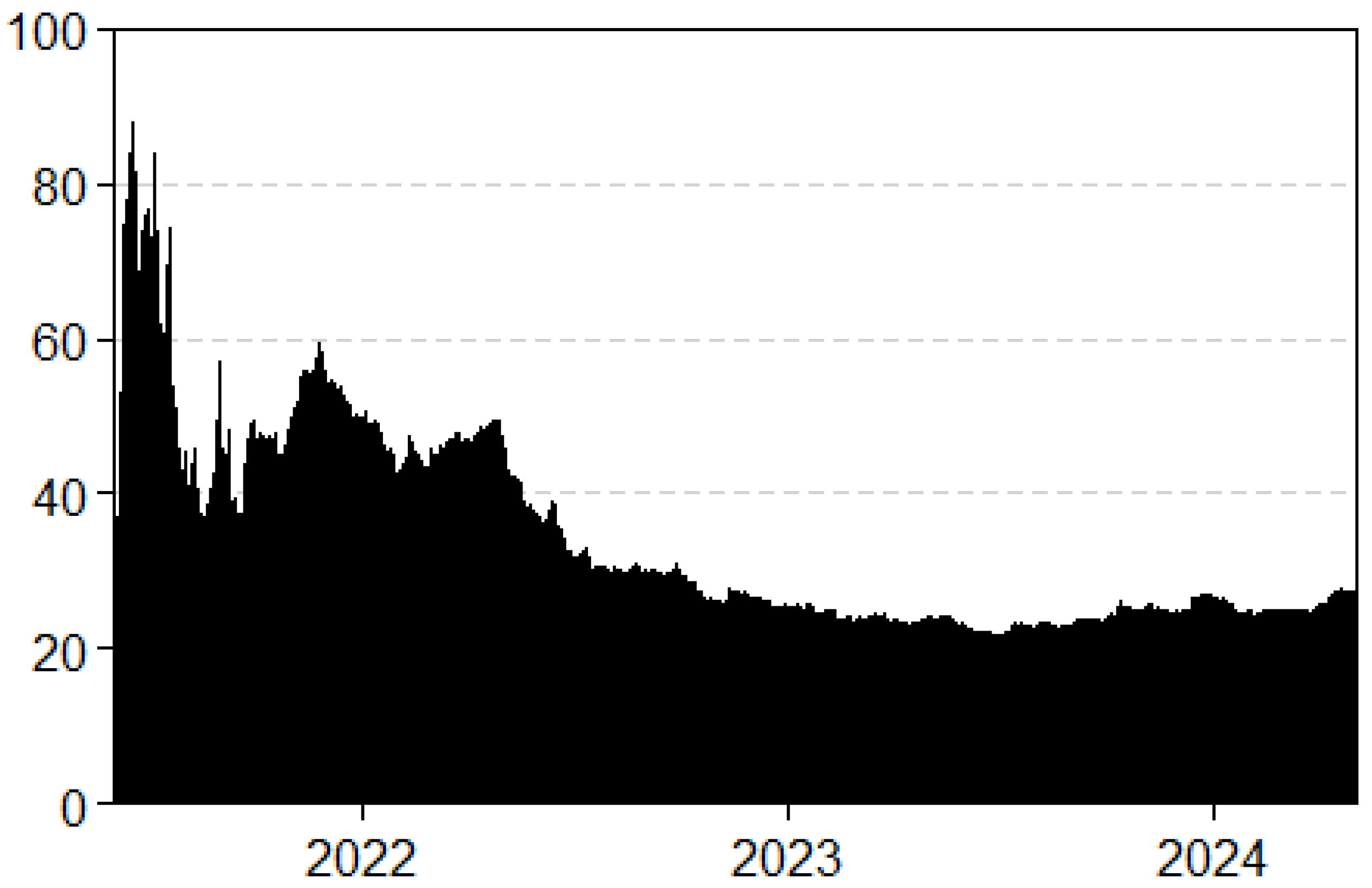
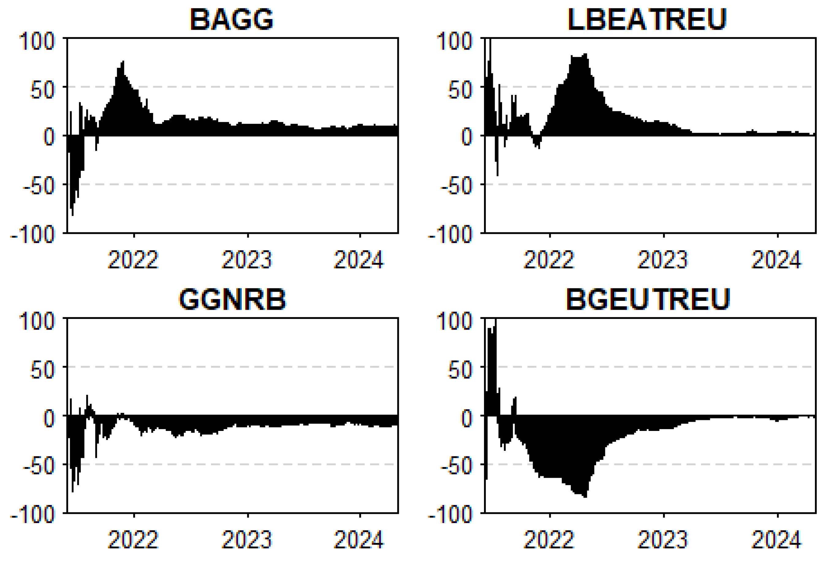
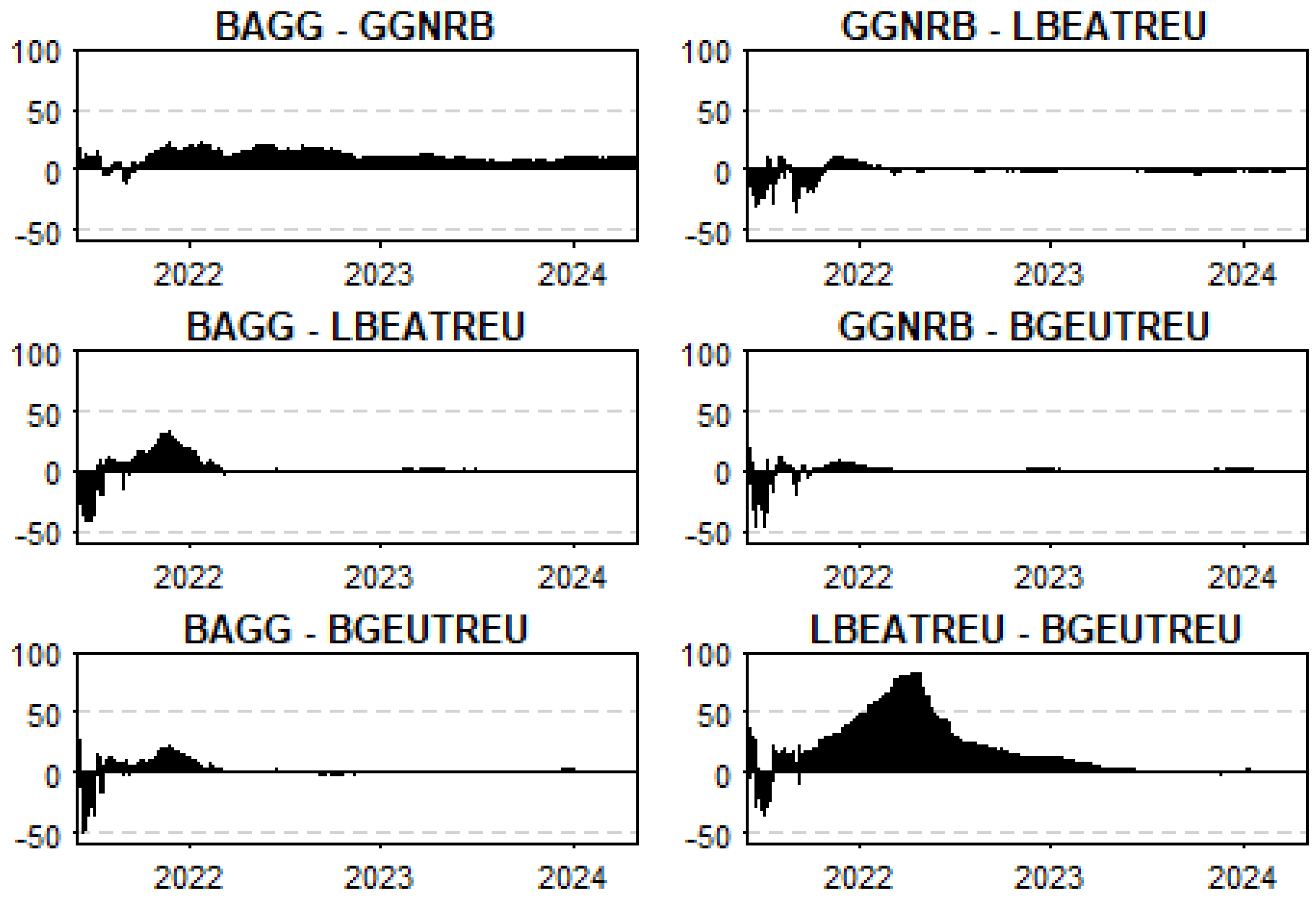
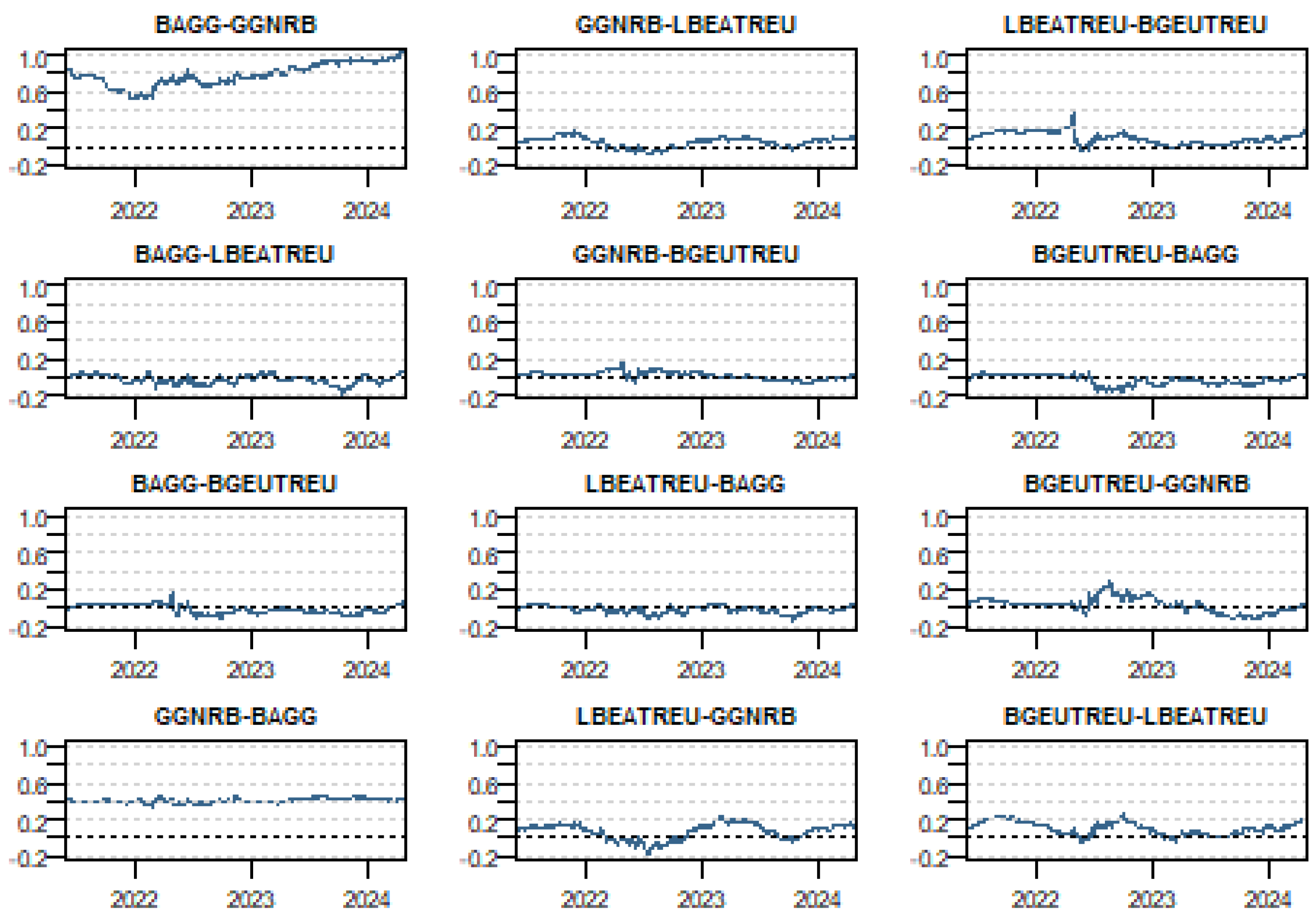
5.1. Dynamic Connectedness

We begin by presenting the results for the average connectedness measures, as shown in Table 2. It is imperative to highlight that the diagonal elements of the table represent idiosyncratic shocks specific to each variable while the off-diagonal elements capture the interactions and spillovers between the different bond types.
The Total Connectedness Index (TCI) results for the four U.S. and E.U. bonds (both black and green) reveal varying degrees of interconnectedness and influence among these assets. The BAGG ETF exhibits the highest TCI at 41.28%, indicating it is the most interconnected and influential, with a notable individual contribution of 114.05% and a positive net connectedness of 14.05%. In contrast, the GGNRB ETF shows a lower TCI of 27.77% and a negative net connectedness of −11.89%, suggesting it is less influential and has a more volatile impact on connectedness. The LBEATREU index shows a TCI of 26.21% with a positive net connectedness of 17.30%, reflecting significant influence and stability, supported by a high individual contribution of 117.30%. Conversely, the BGEUTREU index has the lowest TCI at 6.17% and a negative net connectedness of −19.46%, indicating that it is the least interconnected with minimal stability and impact. These results highlight the varying levels of connectedness and influence each asset has, with BAGG and LBEATREU being the most influential and stable while GGNRB and BGEUTREU exhibit lower levels of impact and stability.
The results of the analysis on the shock transmission and reception across different bond markets show clear roles for each bond type. BAGG (U.S. Aggregate Bonds) emerges as the primary shock transmitter, with the highest values in transmitting its own shocks (72.77) and those affecting other bonds, indicating a significant influence on the broader bond market. In contrast, it receives a smaller proportion of shocks from other bonds (27.23), highlighting its prominent role as a transmitter.
The notable role of BAGG as a shock transmitter during this period speaks to the significant influence of U.S. monetary and fiscal policies. The Federal Reserve’s interest rate adjustments, inflationary pressures, and fiscal stimulus mechanisms associated with the COVID-19 pandemic likely contributed to the increase in market volatility and affected global bond markets. Additionally, political developments, including the 2022 midterm elections and the evolving U.S.–China trade relations, would have influenced BAGG’s role as a major transmitter of market shocks. GGNRB (U.S. Green Bonds), while also a significant receiver of shocks from other bonds (39.66), is a moderate transmitter (60.34) compared to BAGG, reflecting a more balanced yet notable influence in the market. GGNRB’s intermediate role in shock transmission and reception points to the increasing importance of sustainable finance and regulatory changes. The period saw an increased focus on environmental, social, and governance (ESG) criteria, with governments and institutions ramping up investments in green bonds. The U.S. Inflation Reduction Act of 2022 and similar policies likely influenced GGNRB’s moderate shock transmission, reflecting both the growing investor interest in green bonds and the regulatory shifts promoting sustainable investment. LBEATREU (EU Aggregate Bonds) emerges as the largest shock receiver, with an exceptionally high value (91.09), showing its sensitivity to movements in the broader bond market, although it transmits shocks to a lesser extent (4.03).
LBEATREU, as the largest shock receiver, reflects the impact of ongoing economic challenges in Europe, including inflationary pressures, energy crises exacerbated by geopolitical tensions (e.g., the Russia–Ukraine conflict), and the EU’s response to these issues. The significant reception of shocks by LBEATREU highlights the market’s sensitivity to European economic policies and geopolitical events. LBEATREU lower shock transmission points to its role as a primary absorber of market disturbances rather than a source. Similarly, BGEUTREU (E.U. green bonds) is a major receiver of shocks (74.37) but transmits shocks to a relatively smaller extent (3.14), highlighting its limited influence compared to its receiving role. GEUTREU’s high-shock reception aligns with the broader context of E.U. green finance initiatives and regulatory developments. Despite facing significant market shocks, BGEUTREU’s role as a shock transmitter is limited. This points to the E.U.’s Green Deal and other sustainability regulations having impacted green bonds’ market dynamics, making them more sensitive to the broader economic and regulatory environments.
The findings communicate that BAGG plays an important role in transmitting shocks across bond markets while LBEATREU and BGEUTREU are more affected by external shocks, with GGNRB serving an intermediate function. This dynamic interaction among different bond segments is crucial for understanding risk transmission and developing effective portfolio diversification strategies in international bond markets.
The period from June 2021 to May 2024 was characterized by a complex interplay of economic, regulatory, and political developments. The ongoing recovery from the COVID-19 pandemic, combined with inflationary pressures and geopolitical tensions, impacted global financial markets. In addition to evolving investment trends and regulatory changes in sustainable finance, the increase in connectedness and volatility observed in bond markets during this period is partly attributable to these macroeconomic factors. The analysis of shock transmission and reception across different bond markets during this period highlights how various segments of the bond market interact in response to global economic and political developments. BAGG’s role as a key shock transmitter, GGNRB’s intermediate role, and LBEATREU and BGEUTREU as significant shock receivers reflect the broader market dynamics influenced by recent policy changes, economic challenges, and geopolitical events.
We proceed to delve into the more detailed, time-varying results provided by our econometric framework. To begin, we analyze the temporal progression of total connectedness (TCI) as illustrated in Figure 2 Within the framework of our analysis, high values of the TCI indicate significant co-movements within the network, suggesting that the perceived risks associated with the different bond types are becoming more aligned. This alignment reflects a similarity in the levels of market confidence across the bonds in question. In Figure 2, the Total Connectedness Index (TCI) graph within our network highlights significant variations in the interconnectedness of U.S. and European bond markets over the period from mid-2021 to 2024, with these fluctuations closely aligning with key economic and geopolitical crises.
Following the COVID-19 pandemic, starting mid-2021 to early 2022, the TCI showed notable spikes, reflecting the market’s increased volatility and sensitivity to the economic uncertainties, inflation fears, and anticipated changes in monetary policy by the U.S. Federal Reserve. Moving into 2022, the TCI started to decline, suggesting a period of stabilization, with the markets having absorbed the initial shocks. This decline coincided with the period of relative calm after the initial disruptions caused by the Ukraine conflict and energy crisis in Europe, implying that the bond markets were adapting to the new economic realities. By mid-2023 to 2024, the TCI stabilized at a lower level, signifying reduced interconnectedness and volatility in the bond markets. The minor fluctuations during this period reflected the ongoing economic developments such as inflationary pressures and evolving geopolitical situations. These results are broadly consistent with findings by Mensi et al. (2024) and Wang et al. (2024), who also observed increased shock transmission during crisis periods and reduced co-movement during more stable phases. However, unlike Broadstock et al. (2022), who noted stronger connectedness of green bonds across international markets, our results highlight a more regionally asymmetric role of green bonds in the U.S. and E.U., with U.S. green bonds acting as moderate transmitters and E.U. green bonds as receivers.
We now turn to the CUSUM test, which has produced a statistic of 0.713 and a corresponding p-value of 0.689, providing no evidence of structural instability at conventional significance levels. Therefore, we fail to reject the null hypothesis of parameter stability, implying that no statistically significant structural breaks were detected within the sample period. This result suggests that the TVP-VAR/QVAR framework applied in our paper is appropriate as the underlying system exhibits no significant abrupt shifts that would compromise the integrity of the time-varying parameter estimates. While the TVP-VAR model is capable of capturing gradual evolution in parameters, the CUSUM test result further validates that the parameters evolve smoothly without regime-disrupting shocks.
We now shift focus to the progression of total directional connectedness. A distinct strength in our econometric framework is its ability to differentiate and categorize the various bond types in our network as either net transmitters or net receivers of shocks.
When the shaded region in Figure 3 appears in the positive range, it signifies that the corresponding bond type predominantly acts as a shock transmitter within the system. Conversely, when the shaded region falls below zero, the bond index is identified as a net shock receiver. We note that both black U.S. and E.U. bonds retained their net transmitting character throughout the period of analysis, as illustrated in Figure 3, assuming a notable role as transmitters for almost the entire period of study, with the exception of the last quarter of 2021 for the black U.S. bond (BAGG). This can be explained by several economic and political factors during that time like the rising inflation in the United States and Europe, driven by supply chain disruptions, energy price spikes, and high post-pandemic demand. In response, central banks, particularly the Federal Reserve in the U.S., began signaling tighter monetary policies, including tapering asset purchases and anticipating interest rate hikes. This created volatility in bond markets, with government and corporate bonds reacting to the higher expected future interest rates, which typically led to lower bond prices. The BAGG (black U.S. bond) momentarily lost its dominance as a shock transmitter during this period due to the market’s adjustment to the Fed’s new stance before resuming its role once the initial shock of policy change was absorbed. This could also indicate of the unique character of the COVID-19 crisis, which resulted in similar perceptions of risk in both bond markets. These findings align with those of Diebold and Yilmaz (2012) as BAGG’s temporary reduction in shock-transmitting capacity during late 2021 reflects similar dynamics. Not only that, but the last quarter of 2021 saw significant political uncertainty in the U.S. due to debates over the federal debt ceiling. The potential risk of a U.S. default, albeit low, created turbulence in the bond markets.
We now examine the pairwise dynamics, which provide a more detailed understanding of the specific roles and evolving characteristics of each variable over time. To this end, we present pairwise (or bilateral) result, further refining the analysis of the linkages within the bond markets under study (Figure 4).
Throughout the observed period, the U.S. bond markets, represented by BAGG and GGNRB, acted as net transmitters of shocks to European bonds, such as LBEATREU and BGEUTREU. For instance, BAGG consistently influenced GGNRB and both European bonds, particularly during financial stress, suggesting that U.S. markets have a significant impact on global bond dynamics. The intensity of this transmission generally declined over time, suggesting a possible stabilization or adaptation by European markets. Within the European bond market, LBEATREU serves as a net transmitter to BGEUTREU, especially during crises, highlighting the internal dynamics and interconnectedness within the European financial landscape. These results align with findings from other studies on international bond market connectedness like Bekaert et al. (2014), who proved the strong influence of U.S. financial markets on global assets, particularly during crises, due to the U.S.’s prominent role in global capital flows. Kenourgios et al. (2011) similarly emphasize that during periods of financial distress, such as the global financial crisis, the U.S. bond markets transmit shocks to other regions. The observed influence of European bonds, particularly LBEATREU within the European system, aligns with the findings of Bouri et al. (2021), who illustrated significant interconnectedness within regional bond markets, especially in distressed markets. This highlights the interplay of global and regional dynamics in shaping the behavior of bond markets.

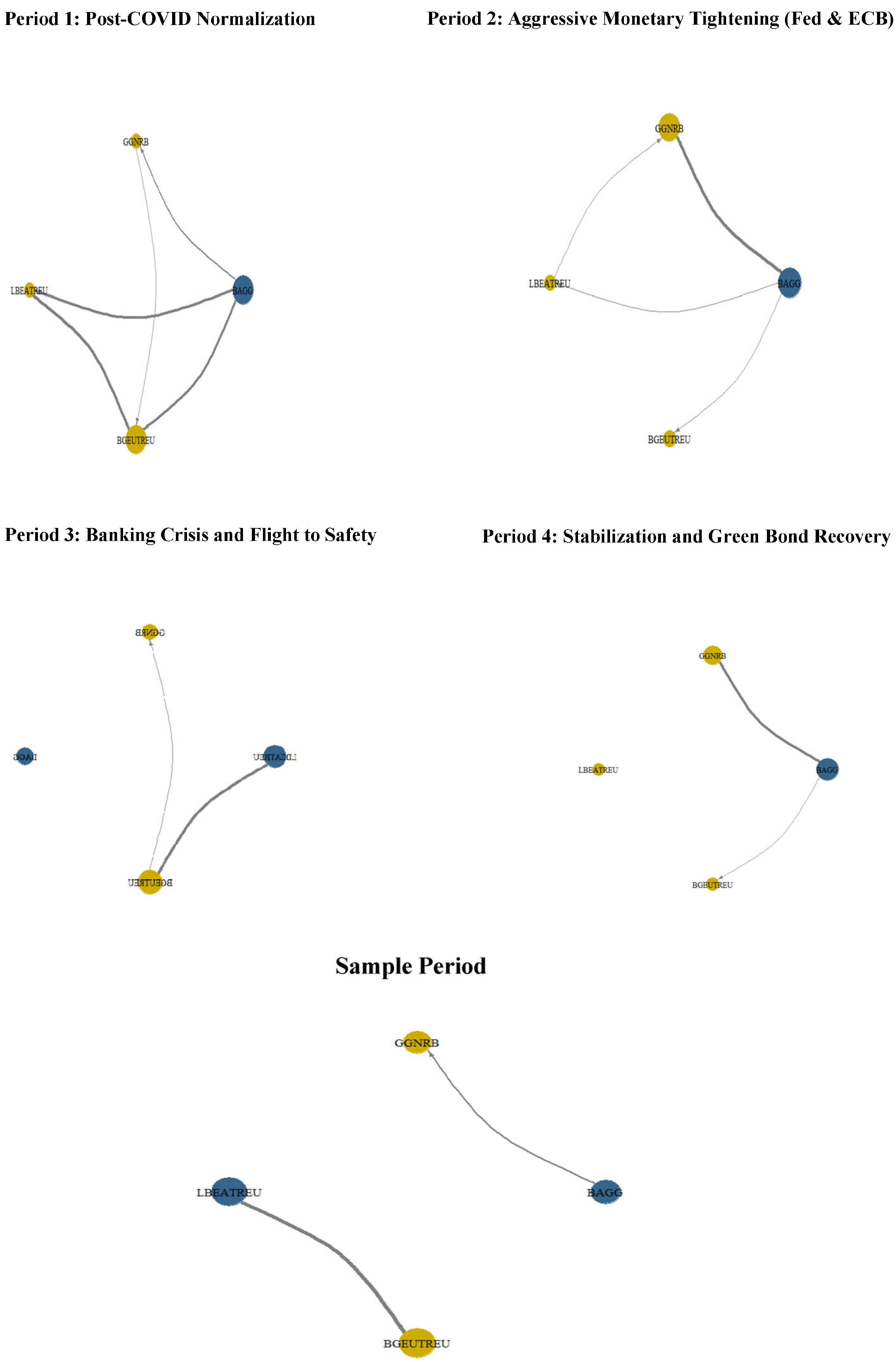
5.2. Network Centrality Analysis

To further explore the systemic importance of each bond index, we convert the pairwise net connectedness matrix (NPDC) into a directed network graph. Each node represents a bond index, and edge directions indicate the direction of net information transmission. Two centrality measures, eigenvector centrality and betweenness centrality, are computed to assess the relative importance and intermediary roles of indices within the spillover structure. Figure 5 illustrates the dynamic spillover networks among U.S. and European green and conventional bond indices across four distinct sub-periods and the full sample period. Each node represents a bond index, with blue nodes denoting green bond indices and yellow nodes representing conventional bond indices. The directed edges capture the direction and intensity of volatility spillovers between indices; thicker lines indicate stronger spillover effects. The figure visually highlights changes in interconnectedness and transmission dynamics during key market phases such as post-COVID normalization, monetary tightening, banking stress, and bond market stabilization.
Overall, the results reveal a dynamic evolution in spillover structures, highlighting shifting leadership and sensitivity across bond markets. During Period 1 (post-COVID normalization), the U.S. conventional bond index (BAGG) emerged as the dominant transmitter of shocks, particularly toward European bond markets. European green bonds (BGEUTREU) were primarily influenced by their conventional counterparts (LBEATREU), confirming the hierarchical dependency of ESG assets on broader fixed-income markets. In Period 2 (monetary tightening), BAGG further consolidated its central position, transmitting to all other indices, particularly U.S. green bonds (GGNRB). A modest feedback loop from GGNRB to BAGG also appeared, indicating increasing bidirectional dynamics within the U.S. market. Meanwhile, Europe remained largely reactive, with limited outward influence. Period 3 (banking crisis) marked a major structural break. BAGG became fully disconnected from the network, reflecting its role as a financial safe haven. European markets showed stronger internal connectedness, particularly from LBEATREU to BGEUTREU, while green bonds on both sides of the Atlantic played mostly passive roles, acting as volatility absorbers during heightened financial stress. Finally, Period 4 (stabilization and green bond recovery) witnessed a reconfiguration of the network. U.S. green bonds (GGNRB) emerged as proactive transmitters, influencing both BAGG and BGEUTREU. Transatlantic linkages resumed while European conventional bonds (LBEATREU) became isolated, signaling a shift in investor focus toward ESG instruments and reduced systemic relevance for traditional European fixed-income assets. In the full sample period, the network appeared relatively sparse and weakly connected. The U.S. conventional bond index (BAGG) transmitted shocks primarily to the U.S. green bond index (GGNRB), indicating a unidirectional spillover within the U.S. market. European indices (LBEATREU and BGEUTREU) remained largely disconnected, showing minimal interaction with U.S. counterparts and with each other. This suggests that over the entire period, systemic influence was concentrated in the U.S. market while European bond indices played a more isolated and passive role, particularly in terms of volatility transmission. The absence of dense connectivity implies low overall integration across transatlantic green and conventional bond markets when viewed over the long run.
These findings are consistent with the results from the connectedness measures (Table 2) and the pairwise connectedness analysis (Figure 4), reinforcing the observed patterns of shock transmission and market segmentation.

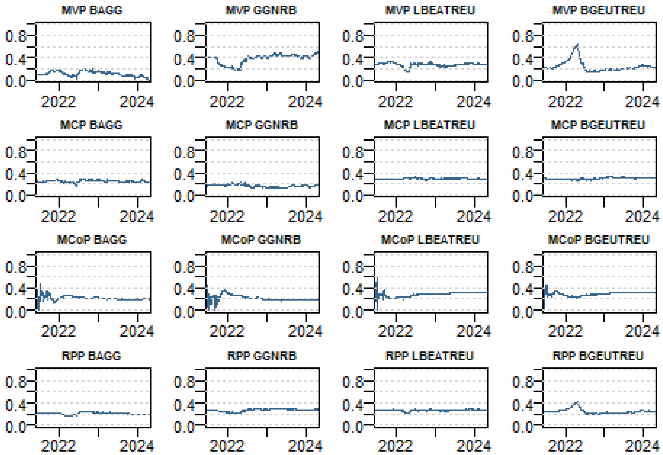
5.3. Dynamic Portfolio

We demonstrate the dynamic allocation of portfolio weights in Figure 6 to provide a clearer understanding of the composition of each portfolio. The figure illustrates the dynamic portfolio weights for four optimization approaches: the MVP, MCP, MCoP, and RPP.
It is clear, from observation, that the composition of the MVP is distinctly different from those of the MCP, RPP, and MCoP. The MCP and MCoP have closely aligned compositions, both with each other and with RPP. This similarity between MCP and MCoP compositions is not entirely unexpected as both are based on the same time-varying variance–covariance matrix. The processes to obtain the final inputs for portfolio calculations, however, differ significantly. The MCP uses a straightforward conversion of the variance–covariance matrix into a correlation matrix whereas the MCoP requires a more complex sequence of computations. The differing transformations make it surprising that the resulting portfolio weights are so closely correlated.
The MVP (Minimum Variance Portfolio) approach shows the most differences in portfolio weights, particularly during periods of market distress, suggesting a higher sensitivity to market conditions. In contrast, the MCP (minimum correlation portfolio) and MCoP (Minimum Connectedness Portfolio) approaches exhibit similar weight allocations, reflecting their common reliance on the variance–covariance matrix, although the MCoP does introduce slightly more variation. The RPP (risk parity portfolio) stands out for its balanced weight distribution across the bonds, confirming its focus on equal risk contributions rather than reacting to short-term market volatility. Overall, while the MVP is sensitive to market fluctuations, the MCP, MCoP, and RPP maintain more stable allocations, with the RPP prioritizing risk parity.
Observing empirical similarities between the MCP and MCoP, we explore their implication on portfolio and risk management. In Table 3, we examine and compare the hedging effectiveness of the four portfolio optimization approaches to provide insights into how different allocation strategies affect asset volatility.
For the Minimum Variance approach, allocating 11% to BAGG, 38% to GGNRB, 27% to LBEATREU, and 24% to BGEUTREU significantly reduces the volatility of these assets by 71%, 56%, 65%, and 74%, respectively. These reductions are statistically significant, with p-values of 0.00 confirming the robustness of the results.
In comparison, the Minimum Correlation approach suggests a different allocation with 25% to BAGG, 16% to GGNRB, 29% to LBEATREU, and 30% to BGEUTREU. This approach also results in volatility reduced by 71%, 56%, 65%, and 74%, similar to the Minimum Variance approach, indicating that the correlations between assets influence risk management outcomes in an equivalent manner.
The Minimum Connectedness approach, with allocations of 21% to BAGG, 21% to GGNRB, 28% to LBEATREU, and 29% to BGEUTREU, yields reductions in volatility by 71%, 56%, 65%, and 74%, reflecting comparable effectiveness in managing risk. These results are statistically significant, highlighting the importance of connectedness in portfolio optimization.
Finally, the Risk Parity approach, which allocates 21% to BAGG, 27% to GGNRB, 27% to LBEATREU, and 25% to BGEUTREU, results in reductions in volatility by 62%, 9%, 39%, and 10%, respectively. These reductions are similarly statistically significant, validating the approach’s efficiency in balancing risk across assets. Each method’s effectiveness in reducing volatility highlights the importance of customized allocation strategies for optimal risk management.
Next, we examine Table 4, which presents the reward-to-volatility (Sharpe) ratios, indicating the expected return per unit of risk for each portfolio. The daily mean return is highest for the RPP, significantly outperforming the other strategies, followed by the MCP, MCoP, and MVP.
In terms of volatility, the RPP exhibits the lowest standard deviation, suggesting a more stable return profile, while the MCP displays the highest risk, followed closely by the MVP and MCoP. Despite the RPP’s strong average return and low volatility, it yields the lowest Sharpe ratio (0.0112), indicating a weak risk-adjusted performance. The highest Sharpe ratio is observed for the MCoP (0.0918), closely followed by the MVP (0.0912) and MCP (0.0910), reflecting more efficient compensation for risk in these portfolios compared to the RPP. From a managerial perspective, this suggests that although the RPP offers high absolute returns, it may not be optimal for investors prioritizing risk-adjusted performance. Portfolios like the MCoP or MVP provide more balanced profiles, making them preferable choices in risk-aware portfolio allocation strategies.
To enrich the hedge effectiveness analysis and better account for tail risk, we computed the Conditional Value at Risk (CVaR) at the 5% and 1% confidence levels for both unhedged and hedged portfolios in the U.S. and Euro green bond markets (Table 5).
For the U.S. market, hedging with black bonds results in a CVaR (5%) of −0.0096 versus −0.0075 for the unhedged green bond portfolio, yielding a ΔCVaR of 0.0021. Similarly, at the 1% level, the CVaR increases from −0.0100 (unhedged) to −0.0124 (hedged), giving a ΔCVaR of 0.0024. These positive differences indicate that the hedge slightly increases exposure to extreme losses. A similar pattern is observed in the Euro market, where the hedged portfolio shows a CvaR (5%) of −0.0082, compared to −0.0098 for the unhedged one, resulting in a ΔCVaR of 0.0016. At the 1% level, the hedged CVaR improves to −0.0105 from −0.0126, with ΔCVaR = 0.0021. These findings suggest that while hedging may reduce average volatility, it could also increase downside risk in extreme scenarios in both markets. This tail-risk analysis, introduced after Equation (15), provides additional insights into the trade-offs involved in using black bonds as hedging instruments against green-bond exposure.
Overall, these findings demonstrate the effectiveness of different strategies in mitigating asset volatility and improving hedging efficiency. Each approach offers unique advantages, with statistically significant reductions in volatility achieved through tailored asset allocations. While these results highlight the potential for effective risk management and diversification within the examined portfolios, it is important to acknowledge that these conclusions are based on specific data and may not universally apply to all scenarios. Future research should further explore these approaches to assess their applicability across different market conditions and asset classes, enabling a holistic understanding of their impact on portfolio performance and resilience.
We follow the analysis of multivariate portfolios, examining bivariate portfolios to evaluate the hedging capacity of green bonds against investments in black bonds for both the U.S. and E.U. markets. Table 6 shows the bivariate portfolio weights for various pairs of assets, BAGG, GGNRB, LBEATREU, and BGEUTREU, alongside their statistical properties. These weights reflect the average allocation to each asset in the pair and how these allocations vary over time. The table also provides additional information on the standard deviation, fifth and ninety-fifth percentiles, hedging effectiveness (HE), and p-values for each pair.
The dynamic bivariate portfolio weight table provides insights into the allocation patterns and risk management effectiveness of various asset pairs: BAGG, GGNRB, LBEATREU, and BGEUTREU. For example, the mean weights reveal that in the BAGG–GGNRB pair, GGNRB typically receives a significantly higher allocation (84%) compared to BAGG (16%). In contrast, the BAGG–LBEATREU and BAGG–BGEUTREU pairs show more balanced allocations, with mean weights of 45% and 49%, respectively. The variability in these allocations is captured by standard deviations ranging from 0.04 to 0.13, indicating the extent of fluctuation in portfolio weights. The fifth and ninety-fifth percentiles further illustrate the range within which these weights fall, highlighting the variability over time. Hedging efficiency (HE) values range from 0.11 to 0.57, reflecting differing levels of effectiveness in mitigating risk. Notably, all results are statistically significant, with p-values of 0.00, confirming that the observed patterns in portfolio allocations are robust and unlikely to change. These findings underscore the importance of dynamic adjustments in asset allocations to optimize risk management and achieve strategic portfolio goals.
The varying allocations between asset pairs demonstrate the portfolio’s commitment to diversification as a risk management strategy. By integrating both green and traditional bonds from different regions, the portfolio seeks to distribute risk and enhance stability. For instance, the higher allocation to GGNRB (green bonds) reflects the growing trends towards environmental, social, and governance (ESG) considerations. This shift is driven by regulatory pressures, increased demand for green investments, and the long-term benefits associated with sustainable assets.
The portfolio’s composition reflects the response to market volatility. During periods of increased volatility, investors tend to adjust their allocations to mitigate risks or take advantage of emerging opportunities. The observed differences in asset weights, particularly in the context of hedging effectiveness, mirrors this ability to adapt to evolving economic conditions. The standard deviation in asset weights further highlights the response to fluctuations in the market, demonstrating how the portfolio seeks to optimize risk exposure.
Our results corroborate those of Abuzayed and Al-Fayoumi (2023) emphasizing the strategic role of green bonds in enhancing portfolio resilience and diversification, particularly during periods of financial distress. Similarly, Ejaz et al. (2022) highlighted the importance of managing market risk and dependence structures between green bonds and other financial markets, showing their potential as effective hedging instruments. Furthermore, the response of the portfolio to market volatility aligns with the insights of Naeem et al. (2023), who demonstrate that adaptive strategies involving green and conventional assets can optimize risk management and improve performance when faced with uncertainty. These findings give validity to the importance of flexibility and ESG integration in modern portfolio management.
The high hedging effectiveness (HE) values indicate the portfolio’s capacity to withstand economic shocks and market volatility. The selection of asset pairs with strong hedging properties aims to stabilize returns and minimize downside risk, ultimately enhancing the portfolio’s performance. Figure 7 illustrates the dynamic hedge ratios across various bond indices, particularly U.S. and European green and black bonds. For example, in the hedge pair BAGG–LBEATREU, the European green bond index (LBEATREU) is used to hedge the risk of the U.S. black bond index (BAGG). The hedge ratio provides insight into the proportion of LBEATREU required to effectively manage the risk associated with BAGG over time. Analyzing these hedge ratios across different bond pairs sheds light on the capability and effectiveness of green bonds as hedging instruments, with certain pairs demonstrating greater stability and others requiring more active management due to fluctuations in the hedge ratios. This comprehensive approach highlights the portfolio’s strategic positioning to simultaneously align sustainability goals and maintain robust risk management practices. These results are consistent with Man et al. (2023), who showed that green bonds contribute to lower hedge ratio volatility and serve as stabilizing assets during financial turbulence. They also complement the findings of Broadstock et al. (2022), who emphasized the value of minimum-connectedness strategies in achieving better risk-adjusted returns in portfolios with high green-bond exposure.
The overall results reveal different levels of stability across different pairs of bonds. For instance, pairs like BAGG–GGNRB display relatively stable hedge ratios, indicating a predictable and consistent relationship between the assets, which can simplify the hedging process. In contrast, pairs such as BGEUTREU–BGGNRB exhibit more fluctuations, suggesting a volatile relationship that requires active management. Green bonds, such as GGNRB (Green U.S.) and LBEATREU (Green E.U.), generally show less volatility compared to black bonds. This is evident in the smoother hedge ratios of certain green bond pairs, highlighting their role in stabilizing portfolios. The relatively stable and sometimes lower hedge ratios in portfolios involving green bonds suggest that these instruments can shield against volatility, thereby enhancing portfolio resilience during periods of market distress. These results contribute to a deeper understanding of the investment choice within bond portfolios and offer practical implications for risk management strategies in the bond market. These findings are in line with those of Man et al. (2023) and Naeem et al. (2021), who also identified green bonds as effective hedging instruments during turbulent periods. However, unlike Broadstock et al. (2022), who observed a strong global role for green bonds across markets, our results emphasize region-specific behavior, particularly the higher hedging stability of U.S. green bonds compared to their E.U. counterparts.
Green bonds offer significant opportunities for portfolio risk management and diversification, especially during periods of high uncertainty. Managers should consider increasing the proportion of green bonds in portfolios where risk mitigation is a priority. The fluctuating hedge ratios observed in some portfolios suggest the need for frequent adjustments to the hedging strategies, and the use of automated or algorithmic tools may enhance real-time tracking and adjustment. Beyond their role in risk mitigation, green bonds also align with ESG (environmental, social, and governance) criteria, adding a layer of stability that should be communicated to stakeholders as a strategic advantage. Portfolios with stable hedge ratios involving green bonds can be positioned as lower-risk investment options, appealing to risk-averse investors or those pursuing long-term capital preservation strategies. In summary, green bonds contribute to both stability and diversification in portfolio management, making them critical considerations in the development of investment strategies that respond to changing market dynamics and sustainability goals.

6. Conclusions

In conclusion, this paper has highlighted the revolutionary role played by green bonds within the changing financial sector, particularly with regard to portfolio risk mitigation and sustainability objectives. As evidenced by our analysis, green bonds both serve as effective hedging instruments and promote diversification in fixed-income portfolios during periods of financial distress. E.U. green bonds, particularly, perform impressively in aligning financial strategies with environmental, social, and governance (ESG) criteria.
The findings contribute to the growing body of literature on sustainable finance by illustrating the interconnectedness and shock transmission dynamics between green and traditional bonds in both the U.S. and E.U. markets. To incorporate sustainability into their portfolios, investors need to understanding these relationships to optimize investment strategies and achieve long-term financial stability.
The implications of the existence of green bonds and ‘greenium’ are far reaching for issuers and investors alike. Establishing well-defined benchmarks will be beneficial to market participants in navigating the complexities of the green bond market. As the demand continues to rise, this paper lays the foundation for further investigation of the dynamics that influence the pricing and issuance of green bonds. The incorporation of green bonds into investment strategies, during a period characterized by climate change challenges, is both an informed financial decision as well as an important step in promoting a sustainable future.
Future research could extend this analysis in several directions. First, incorporating emerging markets could provide insights into whether green bonds perform similarly in less mature financial systems. Second, assessing the role of green bonds across different asset classes (e.g., equities or real estate) could deepen our understanding of their cross-market interactions. Third, evaluating the long-term effects of new regulatory initiatives—such as the E.U. Green Taxonomy or the SEC’s climate disclosure rules—could offer insights into how policy shapes connectedness and pricing dynamics. Finally, integrating investor behavior or sentiment data could enrich the interpretation of green bonds’ evolving role in sustainable portfolio strategies. Ultimately, incorporating green bonds into investment frameworks during a time of climate and economic uncertainty is both a forward-looking financial strategy and a commitment to global sustainability.

Funding

This research received no external funding.

Institutional Review Board Statement

Not applicable.

Informed Consent Statement

Not applicable.

Data Availability Statement

The original contributions presented in this study have been included in the article. Further inquiries can be directed to the corresponding author.

Conflicts of Interest

The authors declare no conflict of interest.

References

  1. Abuzayed, B., & Al-Fayoumi, N. (2023). Diversification and hedging strategies of green bonds in financial asset portfolios during the COVID-19 pandemic. Applied Economics, 55(36), 4228–4238. [Google Scholar] [CrossRef]
  2. Antonakakis, N., Chatziantoniou, I., & Gabauer, D. (2020). Refined measures of dynamic connectedness based on time-varying parameter vector autoregressions. Journal of Risk and Financial Management, 13(4), 84. [Google Scholar] [CrossRef]
  3. Antonakakis, N., Chatziantoniou, I., & Gabauer, D. (2021). The impact of Euro through time: Exchange rate dynamics under different regimes. International Journal of Finance & Economics, 26(4), 5176–5194. [Google Scholar]
  4. Arat, E., Hachenberg, B., Kiesel, F., & Schiereck, D. (2023). Greenium, credit rating, and the COVID-19 pandemic. Journal of Asset Management, 24, 547–557. [Google Scholar] [CrossRef]
  5. Aynur, A., David, C. B., Xiaoqi, C., & Dong, W. (2019). Time-varying parameter energy demand functions: Benchmarking state-space methods against rolling-regressions. Energy Economics, 82, 26–41. [Google Scholar]
  6. Bachelet, M. J., Becchetti, L., & Manfredonia, S. (2019). The green bonds premium puzzle: The role of issuer characteristics and third-party verification. Sustainability, 11(4), 1098. [Google Scholar] [CrossRef]
  7. Bekaert, G., Ehrmann, M., Fratzscher, M., & Mehl, A. (2014). The global crisis and equity market contagion. The Journal of Finance, 69(6), 2597–2649. [Google Scholar] [CrossRef]
  8. Bouri, E., Jain, A., Roubaud, D., & Kristoufek, L. (2021). Cryptocurrency market contagion during the COVID-19 crisis. Finance Research Letters, 38, 101620. [Google Scholar]
  9. Broadstock, D. C., Chatziantoniou, I., & Gabauer, D. (2022). Minimum connectedness portfolios and the market for green bonds: Advocating socially responsible investment (SRI) activity. In C. Floros, & I. Chatziantoniou (Eds.), Applications in energy finance (pp. 217–253). Springer. [Google Scholar]
  10. Brown, R. L., Durbin, J., & Evans, J. M. (1975). Techniques for testing the constancy of regression relationships over time. Journal of the Royal Statistical Society. Series B (Methodological), 37, 149–192. [Google Scholar] [CrossRef]
  11. Christoffersen, P., Errunza, V., Jacobs, K., & Jin, X. (2014). Correlation dynamics and international diversification benefits. International Journal of Forecasting, 30(3), 807–824. [Google Scholar] [CrossRef]
  12. Contractor, D., Balli, F., & Hoxha, I. (2023). Market reaction to macroeconomic announcements: Green vs. conventional bonds. Applied Economics, 55(15), 1637–1662. [Google Scholar] [CrossRef]
  13. Diebold, F. X., & Yilmaz, K. (2009). Measuring financial asset return and volatility spillovers, with application to global equity markets. Economic Journal, 119(534), 158–171. [Google Scholar] [CrossRef]
  14. Diebold, F. X., & Yilmaz, K. (2012). Better to give than to receive: Predictive directional measurement of volatility spillovers. International Journal of Forecasting, 28(1), 57–66. [Google Scholar] [CrossRef]
  15. Diebold, F. X., & Yılmaz, K. (2014). On the network topology of variance decompositions: Measuring the connectedness of financial firms. Journal of Econometrics, 182(1), 119–134. [Google Scholar] [CrossRef]
  16. Ederington, L. H. (1979). The hedging performance of the new futures markets. The Journal of Finance, 34(1), 157–170. [Google Scholar] [CrossRef]
  17. Ejaz, R., Ashraf, S., Hassan, A., & Gupta, A. (2022). An empirical investigation of market risk, dependence structure, and portfolio management between green bonds and international financial markets. Journal of Cleaner Production, 365, 132666. [Google Scholar] [CrossRef]
  18. Flammer, C. (2021). Corporate green bonds. Journal of Financial Economics, 142(2), 499–516. [Google Scholar] [CrossRef]
  19. Guo, D., & Zhou, P. (2021). Green bonds as hedging assets before and after COVID: A comparative study between the US and China. Energy Economics, 104, 105696. [Google Scholar] [CrossRef]
  20. Han, Y., & Li, J. (2022). Should investors include green bonds in their portfolios? Evidence for the USA and Europe. International Review of Financial Analysis, 80, 101998. [Google Scholar] [CrossRef]
  21. Huynh, T. L. D. (2022). When ‘green’ challenges ‘prime’: Empirical evidence from government bond markets. Journal of Sustainable Finance and Investment, 12(3), 375–388. [Google Scholar] [CrossRef]
  22. Imran, Z. A., & Ahad, M. (2023). Safe-haven properties of green bonds for industrial sectors (GICS) in the United States: Evidence from the COVID-19 pandemic and Global Financial Crisis. Renewable Energy, 210, 408–423. [Google Scholar] [CrossRef]
  23. Karpf, A., & Mandel, A. (2018). The changing value of the ‘green’ label on the US municipal bond market. Nature Climate Change, 8(2), 161–165. [Google Scholar] [CrossRef]
  24. Kenourgios, D., Samitas, A., & Paltalidis, N. (2011). Financial crises and stock market contagion in emerging markets. International Review of Economics & Finance, 20(3), 528–541. [Google Scholar]
  25. Khamis, M., & Aassouli, D. (2023). The eligibility of green bonds as safe haven assets: A systematic review. Sustainability, 15(8), 6841. [Google Scholar] [CrossRef]
  26. Khan, S. A. R., Sharif, A., Golpîra, H., & Kumar, A. (2019). A green ideology in Asian emerging economies: From environmental policy and sustainable development. Sustainable Development, 27, 1063–1075. [Google Scholar] [CrossRef]
  27. Lichtenberger, A., Braga, J. P., & Semmler, W. (2022). Green bonds for the transition to a low-carbon economy. Econometrics, 10(1), 11. [Google Scholar] [CrossRef]
  28. Maillard, S., Roncalli, T., & Teïletche, J. (2010). The properties of equally weighted risk contributions portfolios. The Journal of Portfolio Management, 36(4), 60–70. [Google Scholar] [CrossRef]
  29. Man, Y., Zhang, S., & Liu, J. (2023). Dynamic connectedness, asymmetric risk spillovers, and hedging performance of China’s green bonds. Finance Research Letters, 56, 103295. [Google Scholar] [CrossRef]
  30. Markowitz, H. M. (1959). Portfolio selection: Efficient diversification of investments. Yale University Press. [Google Scholar]
  31. Mensi, W., Selmi, R., Al-Kharusi, S., Belghouthi, H. E., & Kang, S. H. (2024). Connectedness between green bonds, conventional bonds, oil, heating oil, natural gas, and petrol: New evidence during bear and bull market scenarios. Resources Policy, 91, 104888. [Google Scholar] [CrossRef]
  32. Mohammed, K. S., Bouri, E., Hunjra, A. I., & Yan, Y. (2024). The heterogeneous reaction of green and conventional bonds to exogenous shocks and the hedging implications. Journal of Environmental Management, 364, 121423. [Google Scholar] [CrossRef]
  33. Naeem, M. A., Farid, S., Ferrer, R., & Shahzad, S. J. H. (2021). Comparative efficiency of green and conventional bonds pre-and during COVID-19: An asymmetric multifractal detrended fluctuation analysis. Energy Policy, 153, 112285. [Google Scholar] [CrossRef]
  34. Naeem, M. A., Karim, S., & Tiwari, A. K. (2023). Risk connectedness between green and conventional assets with portfolio implications. Computational Economics, 62(4), 609–637. [Google Scholar] [CrossRef] [PubMed]
  35. Peng, G., Ding, J., Zhou, Z., & Zhu, L. (2023). Measurement of spillover effect between green bond market and traditional bond market in China. Green Finance, 5(4), 538–561. [Google Scholar] [CrossRef]
  36. Primiceri, G. E. (2005). Time varying structural vector autoregressions and monetary policy. The Review of Economic Studies, 72(3), 821–852. [Google Scholar] [CrossRef]
  37. Reboredo, J. C., & Ugolini, A. (2020). Price connectedness between green bond and financial markets. Economic Modelling, 88, 25–38. [Google Scholar] [CrossRef]
  38. Sharpe, W. F. (1966). Mutual fund performance. The Journal of Business, 39(1), 119–138. [Google Scholar] [CrossRef]
  39. Tsoukala, A., & Tsiotas, G. (2021). Assessing green bond risk: An empirical investigation. Green Finance, 3(2), 222–252. [Google Scholar] [CrossRef]
  40. Wang, M.-C., Jiang, P., & Chang, T. (2024). Re-examining China and the U.S.’s respective green bond markets in extreme conditions: Evidence from quantile connectedness. North American Journal of Economics and Finance, 75, 102286. [Google Scholar] [CrossRef]
  41. Xu, D., Hu, Y., Corbet, S., & Lang, C. (2024). Return connectedness of green bonds and financial investment channels in China: Implications for hedging and regulation. Research in International Business and Finance, 70, 102329. [Google Scholar] [CrossRef]
  42. Yousfi, M., & Bouzgarrou, H. (2024). Exploring interconnections and risk evaluation of green equities and bonds: Fresh perspectives from TVP-VAR model and wavelet-based VaR analysis. China Finance Review International, 15(1), 117–139. [Google Scholar] [CrossRef]
  43. Zerbib, O. D. (2019). The effect of pro-environmental preferences on bond prices: Evidence from green bonds. Journal of Banking & Finance, 98, 39–60. [Google Scholar]
  44. Zhao, M., & Park, H. (2024). Quantile time-frequency spillovers among green bonds, cryptocurrencies, and conventional financial markets. International Review of Financial Analysis, 93, 103198. [Google Scholar] [CrossRef]
Figure 1. Time Path Yield Bonds. Green and Black Bond Series.
Ijfs 13 00106 g001
Figure 2. Dynamic total connectedness. Results are based on a TVP-VAR (0.99, 0.99) with one lag.
Ijfs 13 00106 g002
Figure 3. NET total directional connectedness. Results are based on a TVP-VAR (0.99, 0.99) with one lag.
Ijfs 13 00106 g003
Figure 4. Net pairwise directional connectedness. Results are based on a TVPVAR (0.99, 0.99) with one lag.
Ijfs 13 00106 g004
Figure 5. Dynamic spillover networks across U.S. and European green and conventional bond indices: a sub-period analysis. Notes: Period 1: June 2021 to February 2022; Period 2: February 2022 to September 2022; Period 3: October 2022 to March 2023; Period 4: March 2023 to May 2024.
Ijfs 13 00106 g005
Figure 6. Dynamic multivariate portfolio weights. Notes Results are based on the time-varying variance-covariance matrices retrieved from the TVP-VAR (0.99, 0.99) with one lag. MVP refers to the minimum variance portfolio, MCP refers to the minimum correlation portfolio, RPP refers to the risk-parity portfolio, and MCoP to minimum connectedness portfolio).
Ijfs 13 00106 g006
Figure 7. Dynamic hedge ratio bivariate portfolios.
Ijfs 13 00106 g007
Table 1. Bonds’ Returns Series Summary Statistics.
BAGGGGNRBLBEATREUBGEUTREU
Mean−0.00024−0.00021−0.000183−0.000221
Std. Dev.0.0043440.0035290.00396050.004605
Skewness0.0850.174 *0.460 ***0.393 ***
(0.342)(0.053)(0.000)(0.000)
Ex. Kurtosis1.132 ***0.939 ***1.473 ***1.508 ***
(0.000)(0.000)(0.000)(0.000)
JB40.160 ***30.730 ***92.328 ***88.574 ***
(0.000)(0.000)(0.000)(0.000)
ERS−8.746−11.032−8.710−8.139
(0.000)(0.000)(0.000)(0.000)
Q (20)18.824 **9.8729.91511.616
(0.028)(0.519)(0.514)(0.343)
Q2 (20)23.738 ***23.795 ***125.039 ***136.198 ***
(0.003)(0.003)(0.000)(0.000)
KendallBAGGGGNRBLBEATREUBGEUTREU
BAGG1.000 ***0.316 ***−0.015−0.005
GGNRB0.316 ***1.000 ***0.0380.012
LBEATREU−0.0150.0381.000 ***0.088 ***
BGEUTREU−0.0050.0120.088 ***1.000 ***
Notes: ***, **, * denote significance at 1%, 5%, and 10% significance levels.
Table 2. Averaged dynamic connectedness.
BAGGGGNRBLBEATREUBGEUTREUFROM
BAGG72.7723.322.271.6427.23
GGNRB34.1160.343.472.0839.66
LBEATREU4.032.4391.092.458.91
BGEUTREU3.142.0220.4774.3725.63
TO41.2827.7726.216.17101.43
Inc.Own114.0588.11117.3080.54cTCI/TCI
NET14.05−11.8917.30−19.4633.81/25.36
NPT3.000.002.001.00
Notes: Inc.Own (Including Own): Refers to the sum of “From” and the corresponding diagonal element (own variance share) for each variable, i.e., it reflects the total forecast error variance explained including own contributions. NET: Calculated as the difference between “TO” and “FROM”, this column measures the net directional connectedness for each variable. A positive value indicates a net transmitter while a negative value indicates a net receiver. NPT (Net Pairwise Transmitter): Represents the number of pairwise relationships in which a given variable acts as a net transmitter of shocks.
Table 3. Dynamic Multivariate Portfolio Weights.
Minimum Variance approach
MeanStd. Dev.5%95%HEp-value
U.S. Black «BAGG»0.110.040.040.170.710.00
U.S. Green «GGNRB»0.380.080.200.470.560.00
EU Black «LBEATREU»0.270.030.200.320.650.00
EU Green «BGEUTREU»0.240.100.150.500.740.00
Minimum Connectedness approach
MeanStd. Dev.5%95%HEp-value
U.S. Black «BAGG»0.210.040.170.270.710.00
U.S. Green «GGNRB»0.210.050.170.320.560.00
EU Black «LBEATREU»0.280.040.220.310.650.00
EU Green «BGEUTREU»0.290.030.230.320.740.00
Minimum Correlation approach
MeanStd. Dev.5%95%HEp-value
U.S. Black «BAGG»0.250.020.220.280.710.00
U.S. Green «GGNRB »0.160.020.130.200.560.00
EU Black «LBEATREU»0.290.010.280.310.650.00
EU Green «BGEUTREU»0.300.020.270.320.740.00
Risk Parity approach
MeanStd. Dev.5%95%HEp-value
U.S. Black «BAGG»0.210.020.180.240.720.00
U.S. Green «GGNRB»0.270.020.220.290.580.00
EU Black «LBEATREU»0.270.010.240.280.660.00
EU Green «BGEUTREU»0.250.040.210.360.750.00
Table 4. Sharpe Ratios.
MVPMCoPMCPRPP
Mean0.00021144550.00021187060.00021480910.002308136
Sd.Dev.0.0023185060.0023090530.0023603520.0002141154
SR0.091199040.091756520.091007240.01122623
Table 5. Conditional Value at Risk.
CVaR (5%) UnhedgedCVaR (5%) HedgedΔCVaR 5%CVaR (1%) UnhedgedCVaR (1%) HedgedΔCVaR 1%
U.S. Bonds−0.75%−0.87%+0.12%−1.05%−1.2%+0.14%
E.U. Bonds−0.98%−0.82%+0.16%−1.26%−1.05%+0.21%
Table 6. Dynamic Bivariate Portfolio Weights.
MeanStd. Dev.5%95%HEp-Value
BAGG–GGNRB0.160.090.030.320.410.00
BAGG–LBEATREU0.450.040.390.510.570.00
BAGG–BGEUTREU0.490.110.220.620.470.00
GGNRB–BAGG0.840.090.680.970.110.12
GGNRB–LBEATREU0.610.060.500.700.420.00
GGNRB–BGEUTREU0.650.130.320.760.340.00
LBEATREU–BAGG0.550.040.490.610.480.00
LBEATREU–GGNRB0.390.060.300.500.540.00
LBEATREU–BGEUTREU0.550.100.260.630.350.00
BGEUTREU–BAGG0.510.110.380.780.530.00
BGEUTREU–GGNRB0.350.130.240.680.610.00
BGEUTREU–LBEATREU0.450.100.370.740.520.00
Disclaimer/Publisher’s Note: The statements, opinions and data contained in all publications are solely those of the individual author(s) and contributor(s) and not of MDPI and/or the editor(s). MDPI and/or the editor(s) disclaim responsibility for any injury to people or property resulting from any ideas, methods, instructions or products referred to in the content.

