Abstract
Fluctuations in oil prices substantially impact both the real economy and international financial markets. Despite extensive studies on oil market dynamics and overnight momentum, a comprehensive understanding of the link between oil price changes and energy market momentum, as well as their broader influence on global financial markets, remains elusive. This study delves into the intricate mechanics of overnight momentum transmission within financial markets, focusing on its origin in oil price fluctuations and its overarching impact on market dynamics. Employing the quantile VAR method, we analyze daily market data from 3 January 2014 to 17 January 2024. This study emphasizes the significance of overnight momentum on the transmission of volatility, particularly in the tails of the distribution, and highlights the necessity for efficient strategies to govern financial stability. The shale oil revolution, COVID-19, the Russia–Ukraine war, and the Israel–Hamas conflict have significantly impacted the interconnectivity of financial markets on a global scale. It is crucial for policymakers to give priority to the monitoring of the energy market to reduce risks and improve the resilience of the system.
Keywords:
overnight momentum; global financial markets; connectivity variations; asymmetric dynamics; crises JEL Code:
G11; G32; C10; C32; K32
1. Introduction
Globally, crude oil has a substantial influence on various industries and is a crucial factor in energy markets. Further, its price fluctuations significantly impact real economies and international financial markets. The surge in investments in the energy business has led to a significant influx of capital into energy futures, thus amplifying its influence on the economy (e.g., Wen et al. 2012; Jiang and Yoon 2020). This trend, known as the “financialization” of the industry, can be attributed to the stronger link between the energy market and other markets. The latter evolution has a considerable influence on the dynamics of risk hedging and the spillover effects across different asset classes (Adams et al. 2020). Many studies confirm this spillover of returns and volatility among energy and other markets (assets), leading to contagion effects (e.g., Al-Yahyaee et al. 2019; Farid et al. 2021; Jebabli et al. 2022; Mensi et al. 2013).
The relationship between energy prices and financial markets boosts economic policy efficacy, prompting global portfolio managers to seek diverse investment options. Numerous studies (e.g., Ahmed and Huo 2021; Daskalaki and Skiadopoulos 2011; Luo et al. 2023) have demonstrated the popularity of such commodities as a source of investment. Jensen et al. (2000) demonstrate that including commodities and futures investments (especially energy products) in portfolios consisting of equities, bonds, treasury bills, and real estate may effectively mitigate risk via diversification.
Nevertheless, energy prices are volatile, and fluctuations in oil prices significantly influence both the real economy and international financial markets. Policymakers and portfolio managers have recently focused on fluctuations in energy markets. Numerous studies have shown that fluctuations in oil prices significantly influence stock markets (e.g., Batten et al. 2021; Lin and Su 2020a, 2020b; Umar et al. 2021), currency markets (e.g., Chatziantoniou et al. 2023; Fasanya et al. 2021; Hussain et al. 2017; Ji et al. 2019; Zorgati 2023), global financial markets (e.g., Demirer et al. 2020; Mensi et al. 2021), commodity markets (e.g., Guhathakurta et al. 2020; Hung 2021), and real estate markets (e.g., Alola 2021; Mensi et al. 2022; Nazlioglu et al. 2016; Nazlioglu et al. 2020). The spillover phenomenon stems from the heightened interconnection between the returns of asset markets and those of other markets, especially following significant shocks. Research conducted by Silvennoinen and Thorp (2013), Sensoy et al. (2015), and Ewing and Malik (2016) states that volatility and correlation exhibit a strong and consistent relationship throughout time, particularly during periods of financial crises or economic and political instability.
One of the greatest challenges is the overnight momentum that pertains to the changes in the value of assets in financial markets that occur outside of normal trading hours. These changes are typically caused by unexpected news changing investor attitude. These fluctuations provide complexity to market dynamics and volatility (Huang et al. 2021; Lou et al. 2019). The overnight momentum phenomenon is also allied with fluctuations in oil prices, demonstrating the complex relationship between financial markets and commodities (Ming et al. 2023; Wen et al. 2021). Price fluctuations during normal trading hours might have an impact on after-hours trading, since new information or macroeconomic data can affect the pricing of assets. This impact stresses the interdependence and intricacy of financial markets, since the momentum that occurs overnight impacts immediate market responses and extends its control into successive trading days.
To understand the dynamics of the oil market and its effects on global financial markets, it is necessary to consider this overnight momentum phenomenon, which has the potential to either magnify or reverse price movements. The correlation between overnight trading momentum in oil prices and other markets highlights the importance of conducting a comprehensive study that considers both factors to fully understand their collective impact on the real economy and global financial markets.
The research to date has tended to focus on the dynamics of the oil market and interactions with other financial markets during trading hours rather than the link between oil price movements, energy market momentum, and their influence on global financial markets. Wen et al. (2021) is a significant exception to the general lack of thorough investigations into the latter concerns related to energy market momentum. In this context, findings from several studies (Griffin et al. 2003; Grinblatt et al. 1995; Jegadeesh and Titman 2002; Liu et al. 2023b; Bogousslavsky 2021) give insight into the way overnight returns might predict future returns. This is further built upon by Wen et al. (2021), who assess the intraday return predictability of stock markets and apply it to crude oil markets using high-frequency US Oil Fund data from 2006 to 2018. They highlight that only the first half-hour oil market results positively predict later half-hour returns, suggesting that overnight momentum could be the direct result of these changes. Unfortunately, there is a noticeable lack of research on the complex connections between overnight momentum caused by fluctuations in oil prices and how it affects other financial markets.
Therefore, this study examines the transmission mechanisms of the overnight momentum generated by changes in oil prices across financial markets. This study first investigates the degree to which overnight momentum is transferred, offering valuable insights into its cross-market influence. Second, it investigates the influence of market conditions by analyzing changes in the estimated dynamic connectivity under good, bad, and typical market periods. Third, it examines the market that is most vulnerable to overnight momentum and its subsequent impact on overall transmission. Fourth, it examines fluctuations in connectivity during and after major economic and geopolitical events in recent decades. This study thoroughly investigates the changing interconnections within financial markets in response to major global events. To fill this essential gap, our analysis synthesizes current knowledge and contributes to a more thorough understanding of how overnight momentum spreads across multiple financial sectors, starting with fluctuations in oil prices.
The present study clarifies several important points raised in earlier studies. Wen et al. (2021) first established that oil markets can, in fact, have overnight momentum; hence, we are interested in studying how this phenomenon, which occurs in energy markets, might spill over to other markets. An analysis of price fluctuations in the oil market not only enhances scholarly comprehension of the intricate dynamics of the crude oil market, including its patterns of momentum and returns throughout the night, but also offers valuable insights for high-frequency traders and investors who contemplate the inclusion of oil products in their investment portfolios. Furthermore, it offers more comprehensive information for policymakers to help gain a better understanding of the high-frequency trading processes in the oil market.
Additionally, this study used the quantile vector autoregression (VAR) methodology to analyze the significance of overnight momentum in the oil market on market volatility. By analyzing variables at several quantiles, the adopted QVAR approach offers a distinctive econometric instrument for comprehending intricate interactions. The objective is to enhance our comprehension of the interaction between the overnight momentum of the oil market and its impact on overall market volatilities, facilitating well-informed decisions by risk managers, investors, and regulators. Consequently, the quantile VAR method is the suitable method if one seeks to identify the possible nonlinearities, asymmetries, and tail characteristics that the financial markets display when reacting to energy shocks occurring overnight. The quantile VAR model is an improvement over the classic VAR framework that incorporates conditional heteroscedasticity over several quantiles; its purpose is to analyze how overnight momentum affects various areas of distribution, particularly severe occurrences.
Third, we analyze a wide range of markets across distinct categories. Research on financial markets, energy shocks, and inflationary mechanisms suggests that markets are subjected to significant difficulties, resulting in significantly increased risk transmission. This is because these times have not only been associated with health- and economy-related issues but have also been a global concern that has affected every sector of the world (Farid et al. 2021, 2022; Goodell 2020; Naeem et al. 2023b; Naeem and Karim 2021; Topcu and Gulal 2020). Due to these triggered encounters caused by various major economic and geopolitical events, this study further investigates the underlying risk transmission mechanisms in several different financial markets. Examining heterogeneous instead of homogeneous markets has the advantage of revealing prospective investment possibilities for diversification (Appiah et al. 2023; Appiah-Konadu et al. 2022; Naeem et al. 2023a). We select various markets to ensure that the scope of our research is sufficient to draw inferences for both investors and policymakers. Financial markets often refer to stock markets, such as the Morgan Stanley Capital International World Stock Index (MSCI). Our analysis includes the Bloomberg Commodity Index, which offers a proxy for overall commodity market trends. Given the significant levels of trading activity, fluctuations, and frequency of returns in currency markets, we include the US Dollar Index (USDX). We also include the S&P 500 Index, which is commonly used to gauge stock market health. The Real Estate Investment Trust (REIT) is an indirect measure of the real estate market. Finally, market expectations for future volatility are considered through the Volatility Index (VIX), which serves as a proxy for overall market uncertainty and risk sentiment.
This study investigates the level of global market integration in the context of major events, including the shale oil revolution, the COVID-19 pandemic, the Russia–Ukraine conflict, and the Israel–Hamas war. These events have resulted in market fluctuations, particularly those affecting overnight movements in oil markets. Geopolitical concerns disrupt oil supply, prompting traders to make overnight adjustments to their holdings. The lockdown significantly impacted oil demand, causing traders to adjust their portfolios. Moreover, the market mood is influenced by geopolitical events, which in turn, affects traders’ views of risk. Speculative trading intensifies oil price volatility. Detailed knowledge of the risk propagation and directional spillovers stemming from overnight momentum in the oil market may improve portfolio creation and hedging methods. To stabilize international markets during crises, authorities must understand market spillovers and connections, including why and how they arise. Investments are primarily concerned with risk reduction during challenging times. Analyzing such return and volatility spillover strengths and directions might assist hedging strategies and financial risk management, which may improve investment decision-making and enable proper judgment during upward spillovers.
The results offer intriguing findings that enhance existing knowledge and provide specific policy recommendations. We find that overnight momentum in energy markets is vital for propagating shocks to other financial networks. Systemic relevance is crucial to preserve financial stability. Policymakers must ensure the stability of the energy market and implement proactive measures to reduce potential risks. The pervasive characteristics of ON highlight the necessity of implementing proactive measures to strengthen market resilience. In extremely low quantiles, markets exhibit higher levels of interconnectedness, suggesting an escalation in the transmission of shocks during periods of market stress or volatility. Policymakers should improve monitoring and intervention strategies to reduce systemic risk and stabilize financial markets. Therefore, understanding market dynamics and investor behavior is crucial for developing effective policy responses and interventions.
2. Empirical Methodology
This study examines how oil price instabilities cause overnight momentum in financial markets and investigates the transmission, market conditions, market vulnerability, and connectivity variations during and after important economic and geopolitical events. Using a QVAR methodology, this study evaluates market volatility over time periods, attempting to detect potential variations in transmission strength during negative, normal, and positive periods, as highlighted in the literature (e.g., Liu et al. 2023a; Baumöhl and Shahzad 2019; Hanif et al. 2021).
In accordance with Ando et al. (2022), we define quantile VAR specifications by combining Diebold and Yilmaz’s (2012) approach with the VAR technique. By integrating quantiles, specifically those located at the tail of the distribution, the QVAR technique effectively mitigates the influence of data outliers on the behavior of conditional variables, thereby contributing to the enhancement of estimation reliability. In addition, the effectiveness of QVAR can be seen due to its capability of estimating tail risk and handling nonlinear effects, adaptability to market changes, utility in stress testing, and capability of analyzing financial data while controlling for outliers.
We examine the relationship between and at each quantile τ ∈ (0, 1) using Koenker and Bassett’s (1978) quantile regression estimation method, assuming that represents a conditional distribution. The QVAR process for the n-variable and pth order is defined as
In Equation (1), the n-vector of the dependent variable at time t is denoted by . The intercepts and residuals of the n-vector at quantile are represented by and , respectively. This quantile-specific modeling incorporates the matrix containing the lagged coefficients in quantiles, denoted by for . When estimating , it is assumed that the residuals completely adhere to the requirements of the quantile population .
Hence, Equation (1) may be expressed in the following fashion, where the th population-dependent quantile of the response variable is considered.
According to Ando et al. (2022) and Cecchetti and Li (2008), the estimation procedure in Equation (2) has an unrelated regression structure. They argue that if each equation in the model contains comparable variables on the right-hand side, then it is feasible to estimate the model using an equation-by-equation quantile regression.
After defining QVAR(p), we now use the methodology that Diebold and Yilmaz (2012) propose to evaluate the spillover indices for quantile variance decomposition at each quantile (τ). Therefore, Equation (1) can be reformulated as
in addition to
Furthermore, we use the Cholesky factorization technique, which is not influenced by variable ordering, as in Cecchetti and Li (2008), Koop et al. (1996), and Pesaran and Shin (1998). We assume that the shocks are not orthogonalized. To determine the generalized forecast error variance decomposition (GFEVD) of a variable that is affected by several shocks, we use the forecast horizon estimates (H) as follows:
The given forecast error (at horizon H) is represented by , which is the jth variable’s contribution to the ith variable’s variance. The vector of error variances is denoted by , the diagonal element of the jth variable for the matrix is , and the ith element of the vector has the value . As an additional measure, we consider the variance decomposition matrix for each item as follows:
Simultaneously, using GFEVD and the connectivity approach that Diebold and Yilmaz (2012) propose, one may obtain additional connectedness estimates at conditional quantiles that follow the quantiles. The total connectedness index (TCI) may be calculated for each quantile τ. Nonetheless, TCI mainly assesses the impact of risk spillovers across different time series on the overall variation in prediction errors within the sample. The symbol for TCI is
All other indices are directionally related to index via the “FROM” connectivity. We may express it as
The directional connectedness from index to all other indices at quantile is represented by the “TO” connectivity, which may be expressed mathematically as follows:
To further assist the dissection of total connectedness for the shocks coming from and to a particular source, the information provided in Equations (8) and (9) provides two sets of directional spillovers. To compute NET connectivity, Equation (8) is subtracted from Equation (9):
Finally, the net pairwise connectedness is computed using the following formula:
The net pairwise volatility spillovers between financial markets i and j are derived by subtracting the gross risk shocks emitted from market i to market j and vice versa. This is carried out to obtain the net pairwise volatility spillovers.
Furthermore, we use a rolling-window methodology to represent the time-varying characteristics of financial markets in the context of their spillovers.
3. Data Description and Preliminary Analysis
This study analyzes quantile volatility spillovers across different financial markets, accounting for major events, including the shale oil revolution, COVID-19 pandemic, Russia–Ukraine conflict, and Israel–Hamas war. It uses daily market data covering the period from 3 January 2014 to 17 January 2024. The data are obtained from DataStream, and the financial markets analyzed are the MSCI World Stock Index, Bloomberg Commodities Index (Bloomberg), US Dollar Index (USDX), S&P 500 Index (SP500), real estate investment trusts (FTSE), and Volatility Index (VIX).
Following seminal work in the literature (e.g., Zhou and Liu 2022; Lou et al. 2019), the daily overnight momentum is calculated as the log-difference between the previous trading day’s close price and the next adjusted opening price , that is,
where signify the logarithms of opening and closing prices for individual stocks or market portfolios on day t, and denotes the logarithm of closing prices (190) on day .
According to the descriptive data and unit root tests provided in Table 1, overnight, MSCI, FTSE, and S&P 500 exhibited a slight upward trend in their respective markets (positive mean and median changes). Conversely, gas displayed a potential downward trend in natural gas prices as indicated by negative mean and median changes. The rest of the indices (USDX and Bloomberg) had slightly negative means, but their medians suggest a more complex outcome. Further, the financial markets with the highest mean volatility returns are the overnight momentum and SP500. The reason for this extreme volatility is that crude overnight momentum in oil prices has fluctuated widely since the financialization of markets (Naeem et al. 2024), whereas the stock market, represented by SP500, is notoriously unpredictable (Karim et al. 2022a, 2022b; Naeem and Karim 2021). Consequently, both markets exhibit very high levels of volatility compared to other markets, as suggested by skewness and kurtosis. Returns on any financial market do not follow a normal distribution, as evidenced by the excessively high values shown by the Jarque–Bera (JB) of normalcy. The latter is further stressed by IQR and mean deviation statistics. Specifically, overnight momentum, FTSE and USDX experienced moderate price swings, while gas exhibited significant price swings. Finally, according to the ERS unit root test, which shows significantly higher values, the data are stationary. Furthermore, all series exhibit ARCH errors, which support the use of the TVP-VAR model, primarily because of the existence of time-varying covariance.

Table 1.
Descriptive statistics.
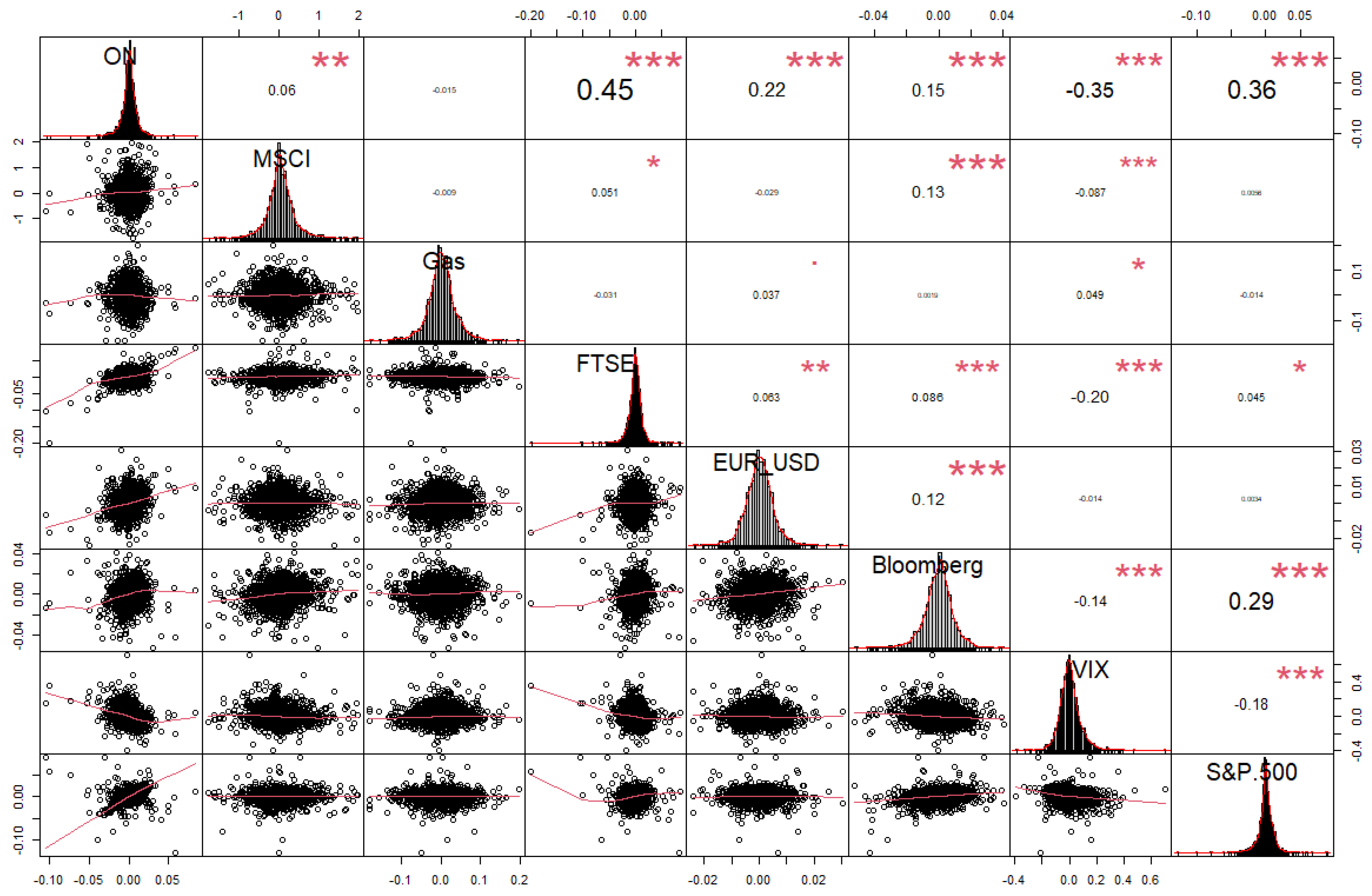
The estimated correlation matrix for the sampled markets is shown in Figure 1. As changes in oil prices might have a major impact on the entire economy, the overnight momentum series and VIX, not surprisingly, have a negative link. Stock prices rise and volatility falls (as measured by the VIX) as oil prices rise, which may indicate increased economic activity. Alternatively, a decrease in oil prices (negative momentum) may signal an uncertain or slowing economy, leading to lower stock prices and greater volatility (VIX). Most correlations are positive, implying that they increase or decrease together and are affected by the same events or risk factors. With a value of 0.45, the coefficient between ON and FTSE is the highest, suggesting a significant correlation between their returns. The correlations between the USDX, Bloomberg, and SP500 are modest, whereas those between the ones with GAS are negligible. Furthermore, the fitted lines of the bivariate scatter plots at the diagonal base show that the series correlation structures vary throughout the joint distribution of returns, implying that a QVAR method is required to characterize all the correlations.
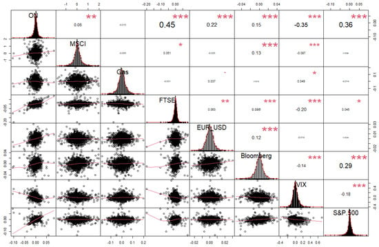
Figure 1.
The correlation matrix chart of the variables. It is important to note that the diagonal illustrates the distribution of each variable. In the bottom right corner of the diagonal are the bivariate scatter plots that have a fitted line shown. The Spearman coefficients and significance level that corresponds to them are located at the top of the diagonal. Additionally, the symbol “***”, “**”, and “*” indicates a significance level of 1%, 5%, and 10%, respectively.
4. Empirical Results
4.1. Static Quantile Connectedness Analysis
The analysis begins with the static quantile connectedness results for the entire sample. Then, the median (τ = 0.5), extreme lower (τ = 0.05), and extreme upper (τ = 0.95) quantiles are presented. The middle, lower, and upper quantiles represent the normal, bearish, and bullish market conditions, respectively.
Table 2 presents the results of the first phase, which analyzes the static connectivity of the entire sample. Notably, with a median TCI of 0.85, series interactions between the series contribute 85% of the variance in the system. However, during periods of market stress, higher TCI values at the 90th and 91st percentiles indicate an even more marked correlation. Additionally, the TCI is greater at the lower end of the distribution compared to the upper end, aligning with findings in prior studies (Patel et al. 2024; Ustaoglu 2023; Jena et al. 2022) that highlight the fact that negative return periods are times of increased risk or uncertainty. This observation suggests that, by ignoring extreme quantiles in favor of average ones, research on overnight momentum and market behavior may have failed to capture the true extent of interconnection. Instead of fixating on typical market conditions, looking at the interdependence of these components in various economic situations is essential.

Table 2.
Static connectedness results (Panel A: full sample).
With a range of 17.61% at the middle quantile to 11% under severe conditions, the analysis reveals that ON has the largest amount of own-variance spillover among all market scenarios. This underlines their influence on future trading sessions. Next, the analysis of directional spillovers shows that ON has a large impact on other network variables, indicating that it is a key indicator or trigger of price swings in linked markets. The row labeled “TO” reveals the findings of the directional spillover to other variables. This indicates that OP has the highest level of spillover (100.8%), whereas the VIX has the lowest level of spillover to the other variables (72.02%) in the network at the median quantile. Additionally, this overflow is greatly amplified at extremely high (102.12%) and low quantiles (107.93%), which aligns with studies in energy economics (e.g., Ustaoglu 2023). This finding suggests limited opportunities for diversification under severe market circumstances. Additionally, the column labeled “FROM” displays the outcomes of directional spillover originating from other sources. Significantly, OP exhibits the lowest degree of spillover from other variables, at approximately 82.39%. The distinction between TO and FROM is NET, which defines whether a series acts as a net transmitter (positive value) or receiver (negative value). The results indicate that OP is the primary transmitter of shocks in the system, particularly in the quantiles examined. Contrarily, VIX is the primary recipient of shocks. Consequently, ON’s shock transmission indicates market sentiment and risk perception. Negative momentum signals an oversupply or geopolitical problems, whereas positive momentum reflects confidence in oil demand. ON’s impact on portfolio dynamics and risk management is highlighted by the revelation of restricted diversification opportunities amid severe market conditions. Finally, understanding ON movements requires a comprehensive understanding of market microstructure and trading patterns outside normal trading hours. This involves evaluating liquidity, trade volumes, and market reactions to news.
4.2. Network Spillovers of Markets
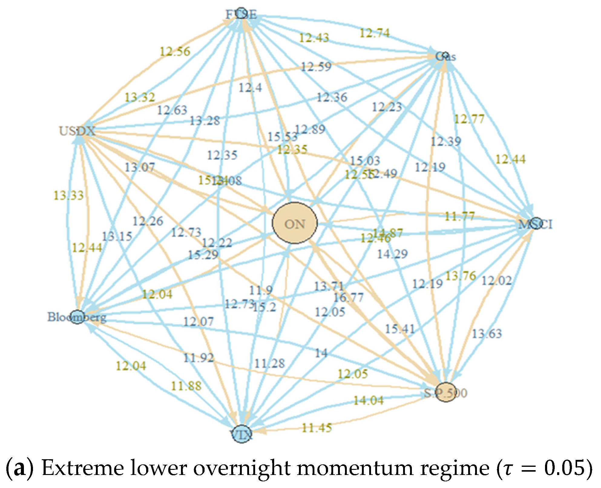
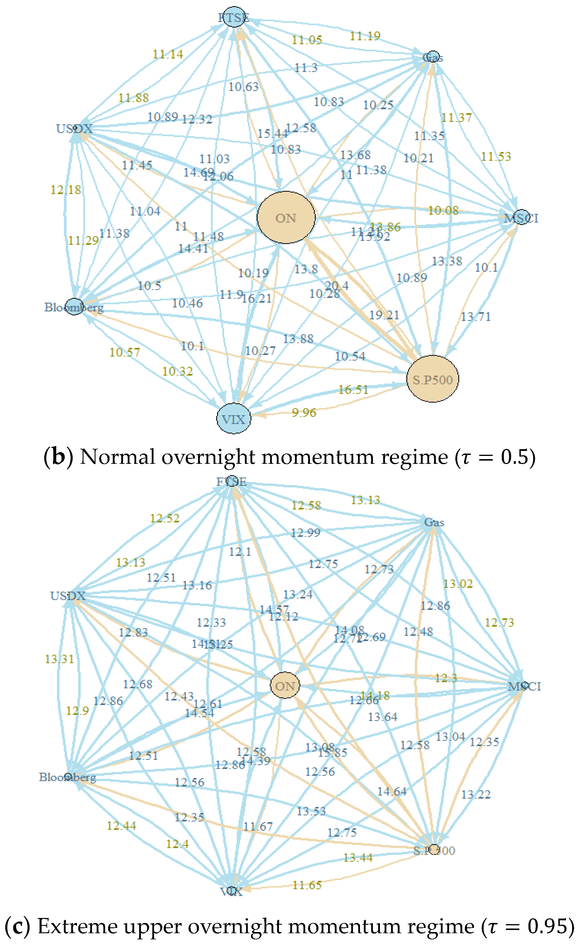
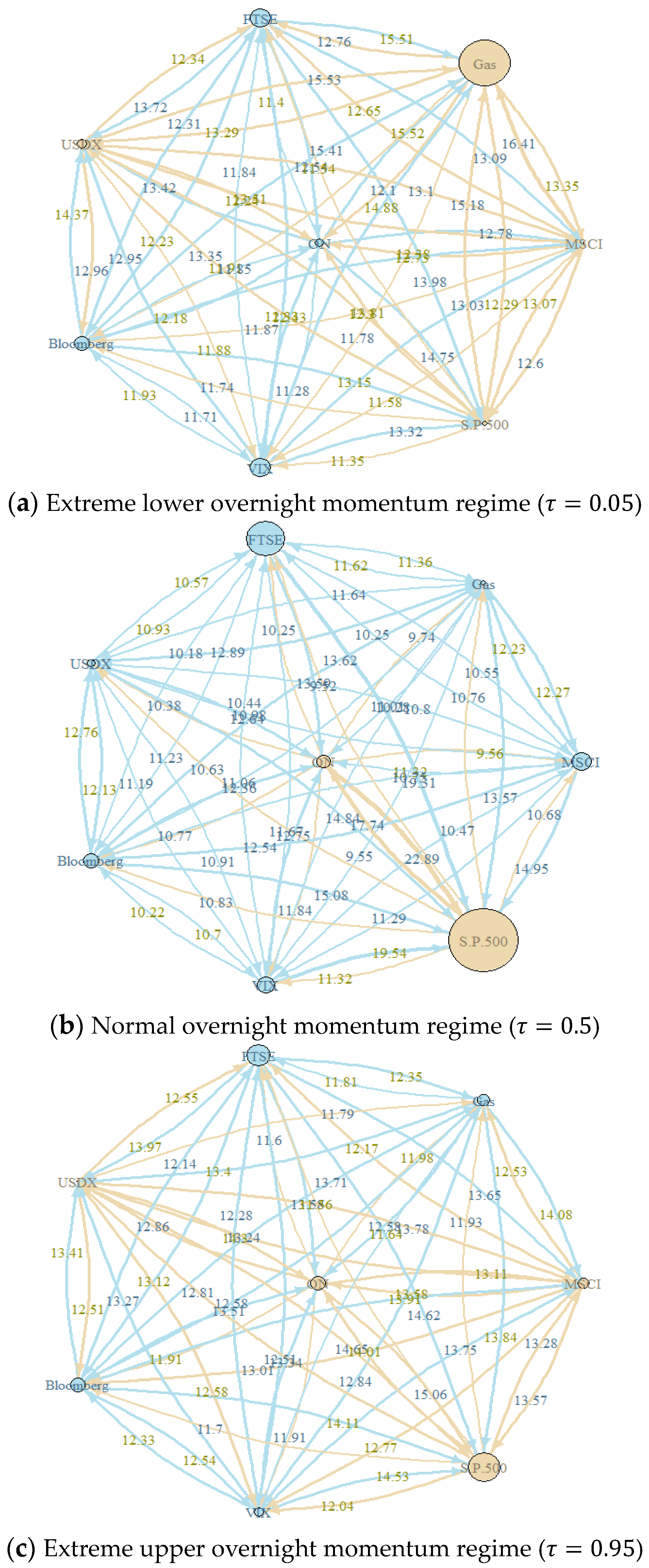
Table 2 shows the overall overnight momentum spillover received and transmitted across financial markets in the network system. This omits the details of the spillover effect on individual markets, making it difficult to identify the market with the most significant impact as a shock transmitter or receiver. The authors analyze the estimated results of the off-diagonal entries of the GFEVD matrix to identify the primary shock transmitters or receivers within the network and determine whether these markets are affected by overnight momentum shocks in the oil markets. The network graphs in Figure 2a–c illustrate the market spillovers throughout the system, where each node indicates the unique traits of its market. Net transmitters are represented by blue nodes, whereas net receivers are represented by khaki nodes. The size of the edges in each picture represents the intensity of the directional spillover, whereas the sizes of the links refer to the amount of spillover sent to or received from all other markets.
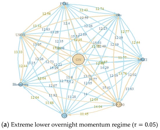
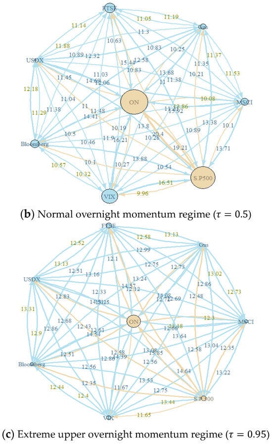
Figure 2.
(a–c) Network connectedness plot (full sample). By using pairwise weighting and utilizing colored borders to indicate connectivity, the directional spillover of the system is shown. Khaki nodes denote major transmitters, whereas blue nodes represent receivers. The accompanying statistics show the risk transmitted or received from other markets, and the edge size shows the level of spillover. The interwoven financial environment and complex web of risk transmission may be better understood with the help of this graphic illustration.
Figure 2b showcases network spillovers during normal times. It appears that all the series are highly interconnected with each other, with ON, followed by SP500, being the largest transmitted shock, while the others act as net receivers. The strongest connection we observe is between ON and SP500, followed by ON and VIX, and then between ON and other markets. Notably, the strong connection between ON and other markets indicates contagion properties. These results emphasize the relevance of the phenomenon of ensuing overnight momentum in the energy market and its impact on the other financial networks, where ON is a significant transmitter of shocks, stressing its systemic relevance because of its interrelated nature. Policymakers must oversee the stability of the energy market (and thus its overnight momentum) to guarantee overall financial stability. The correlation between ON and major indexes such as the S&P 500 and VIX underscores its influence on investor sentiment and market performance. Policymakers may need to adopt legislative measures to reduce the extreme fluctuations and risks that affect the entire system. The contagious nature of ON highlights the need to implement proactive policy measures to strengthen market resilience and reduce the contagion’s impact.
The characteristics of networks at extreme lower quantiles (0.05) are similar to those of the middle networks, except that the USDX plays the role of a net transmitter. Additionally, the linkages between markets seem to be even stronger. Contrarily, the interconnectedness during periods of extreme positive returns is of a relatively different nature, where the transition of positive ON returns to other markets seem to be less intense. This study demonstrates that markets are more linked at extreme quantiles, suggesting a heightened transmission of shocks during times of market stress or volatility. Policymakers should increase monitoring and intervention efforts to reduce systemic risk and stabilize financial markets. The change in the position of the USDX as a net transmitter in the lower quantiles highlights the need to consider the influence of currency market dynamics on exchange rate stability and international trade flows. Understanding the asymmetric dynamics of market connections amid excessively positive returns is crucial for developing effective policy responses and interventions. Another important point to be noted is that market volatility fluctuates between extremely low and high quantiles owing to market dynamics and investor behavior. Investors should be cautious and willing to take risks during times of bad market situations, weak sentiment, and extreme optimism; policymakers should evaluate the effects of these factors on shock propagation and market linkages.
4.3. Do Recent Crises Matter?
Prior to this part, asymmetric market connections are shown by the QVAR-TVP model. During high returns, there are more interconnections, but positive overnight momentum lessens the effect on other markets. During times of market stress and volatility, shocks are transmitted more effectively. This finding aligns with economic theory, which suggests that market volatility fluctuates between the lowest and greatest quantiles because of investor behavior and market dynamics. Thus, governments must increase their monitoring and intervention efforts to reduce systemic risk and stabilize financial markets. To develop successful policies and interventions, understanding the asymmetric dynamics of market relationships during major events is crucial.
Considering this backdrop, a pertinent issue arises: how has connectivity evolved before, during, and after significant political and economic changes during the past few decades? This study explores how the connections between financial markets evolved in response to significant global events. To address this question, we delve further into this study’s spillover network of sample market connectedness during the more recent major crises. For this, we subsample the dataset. We use the sample start date of 3 January 2014, as the beginning of the shale oil revolution, and 11 March 2020, as the beginning of the COVID-19 pandemic, following the World Health Organization bulletin, as well as Naeem et al. (2023a) and Gunay and Kurtulmuş (2021). According to Abakah et al. (2022), the events surrounding the war between Russia and Ukraine began on 24 February 2022, and are still ongoing. Finally, the continuing Israel–Hamas conflict began on 7 October 2023. The subsamples span the following periods: Panel A covers the shale oil revolution (3 January 2014 to 30 December 2016), Panel B covers the COVID-19 pandemic (lockdown time) (11 March 2020 to 10 March 2021), Panel C covers the Russia–Ukraine conflict (24 February 2022 to 17 January 2024), and Panel D covers the ongoing Israel–Hamas conflict (7 October 2023 to 17 January 2024).
First, we examine the static connectedness during these major events. These findings are quantitatively similar to our full sample period results (Table 2), with the ongoing Israel–Hamas war being an exception. In brief, the TCI at the median quantile suggests that the interactions between the series account for 85% of the variance observed in the system during the shale oil revolution and COVID-19 (Table 3), whereas the TCI is relatively lower during the two ongoing conflicts of Russia–Ukraine (approximately 82%) and the Israel–Hamas war (approximately 79%), as shown in Table 3. Similarly, the TCIs at the 95th and 5th percentiles are higher, suggesting a stronger correlation between these series during periods of severe market circumstances. We find that, at the considered quantiles, ON still has the highest own-variance spillover during both the shale oil revolution and the Russia–Ukraine conflict, but not during both the COVID-19 pandemic and the Israel–Hamas war, where gas takes the lead. Moreover, the row NET suggests that ON is the major risk transmitter in almost every subsample, with two exceptions at the lower quantile during both the COVID-19 and the Israel–Hamas war, where its role becomes a net receiver of a shock.

Table 3.
Static connectedness results.
Together, these findings clarify the deep interconnections that are apparent in economic and financial data during significant events, such as the shale oil revolution, the COVID-19 pandemic, and geopolitical conflicts. This study primarily focuses on overnight momentum in oil markets as a crucial signal. The TCI highlights the major influence of ON, explaining a considerable proportion of the observed variability, ranging from 79% to 85%. The interconnectedness between various factors can be attributed to heightened market sentiment and the uncertainty surrounding oil prices, investors seeking refuge in oil assets amid global turmoil, intensified globalization, the integration of oil markets, and policy responses that impact oil market dynamics. Furthermore, the rapid spread of information has a substantial effect on trading activity in oil markets, which occurs throughout the night. These findings highlight the importance of understanding and effectively controlling risks related to overnight changes in oil markets during times of economic and geopolitical instability. This emphasizes the urgent need for strong policy measures to reduce the risks to global financial markets.
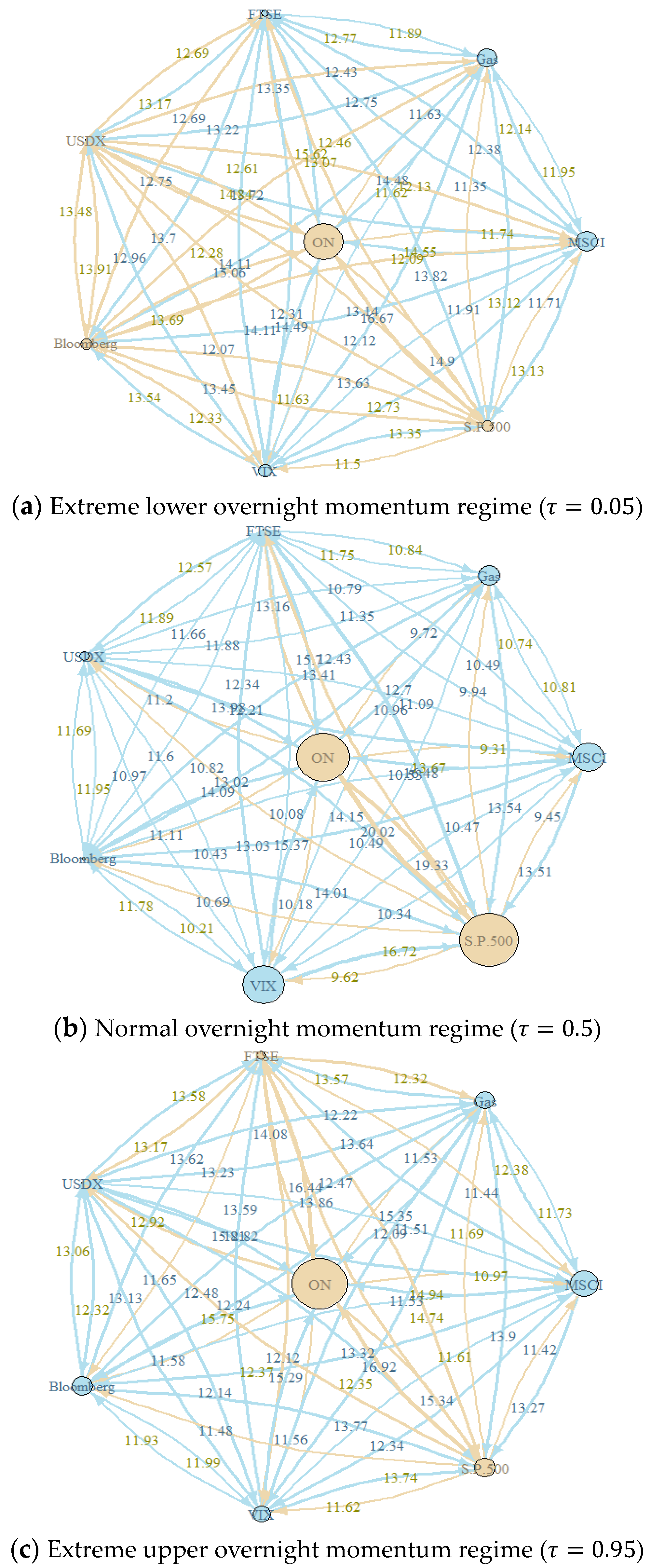
The focus now moves to the off-diagonal elements of the GFEVD matrix to identify important shock transmitters and assess whether these markets are affected by overnight oil market momentum shocks at crucial moments. Figure 3 shows the interconnection of the sample markets during the shale oil boom. The median quantile shows no discernible change in the interconnection of the sample markets between the shale oil revolution period and the overall timeframe, suggesting that overnight momentum does not affect other markets. At the highest quantile of positive momentum, the illustration shows a modest variation, in which both ON and SP500 transmit their shocks to other markets more strongly than observed for the full sample (Figure 2c). Conversely, the intensity of the spillover transition is considerably weaker in the lower quantiles. Additionally, it is intriguing that the USDX and Bloomberg are among the transmitters.
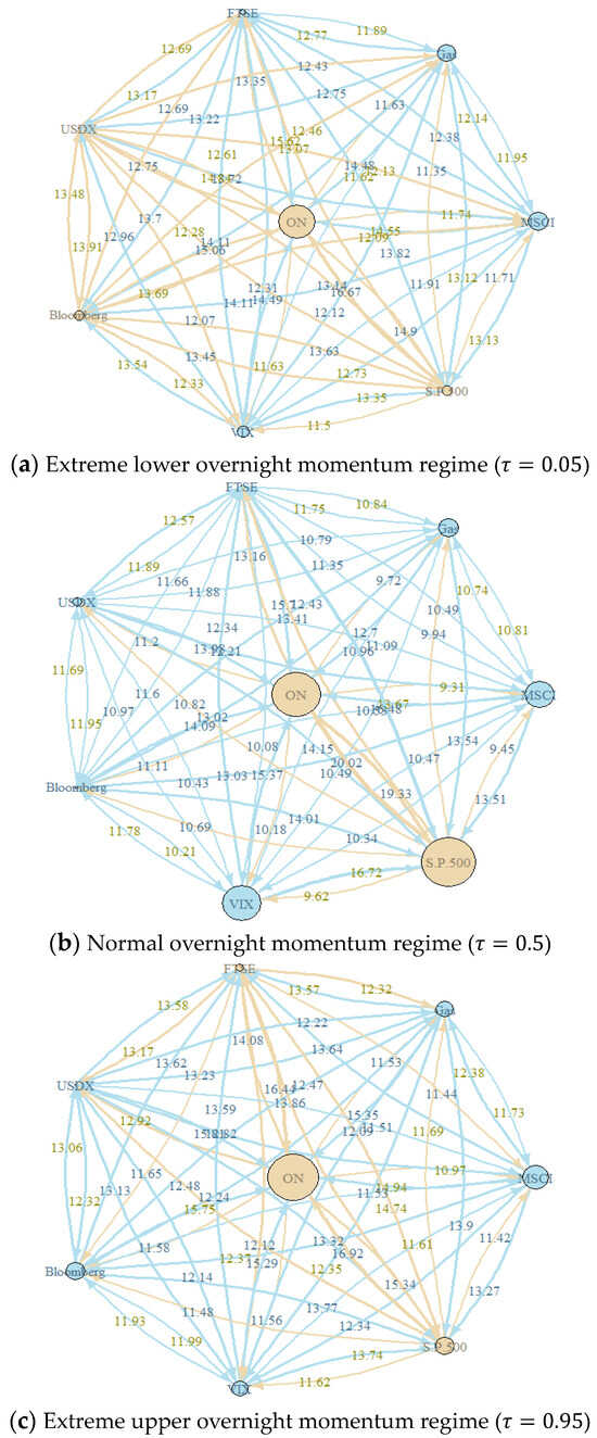
Figure 3.
(a–c) Network connectedness plot (shale oil revaluation period). By using pairwise weighting and utilizing colored borders to indicate connectivity, the directional spillover of the system is shown. Khaki nodes denote major transmitters, whereas blue nodes represent receivers. The accompanying statistics show the risk transmitted or received from other markets, and the edge size shows the level of spillover. The interwoven financial environment and the complex web of risk transmission may be better understood with the help of this graphic illustration.
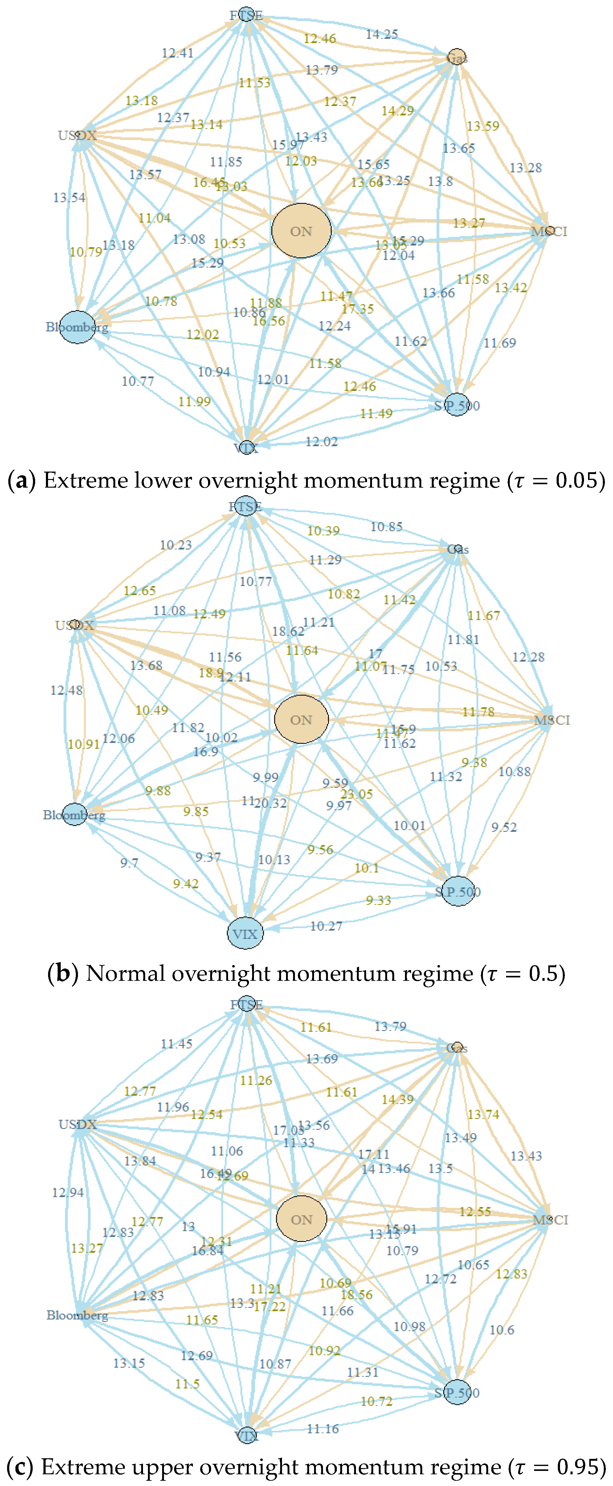
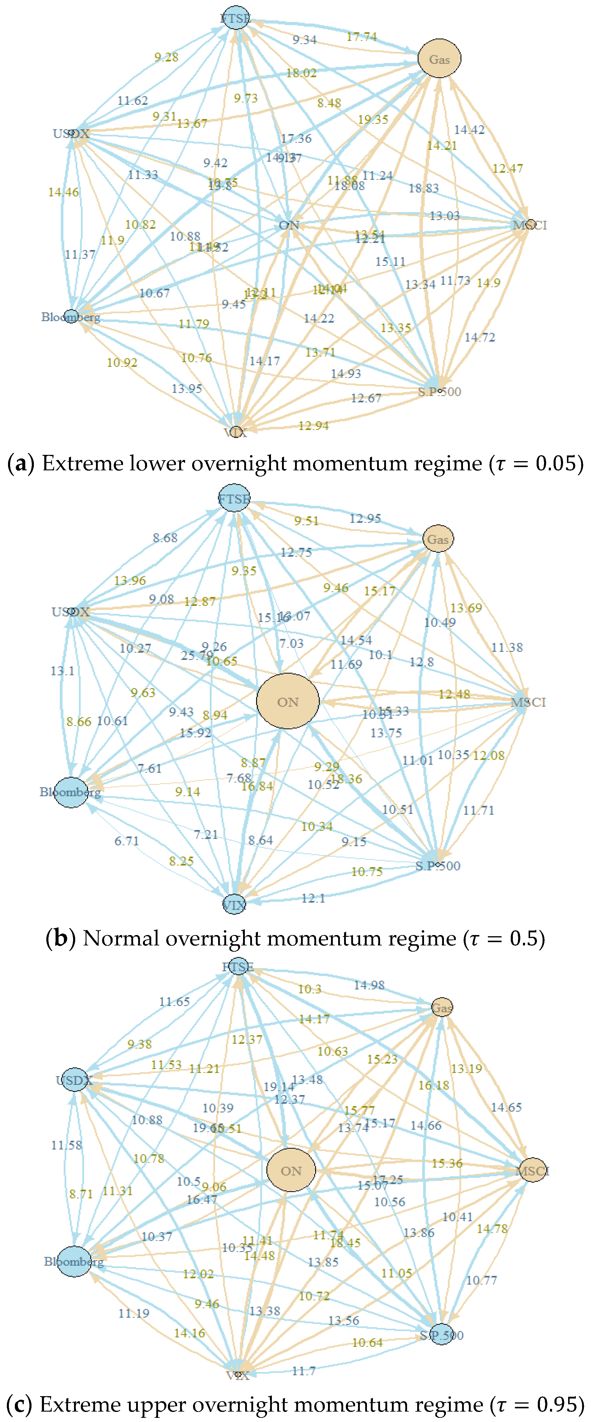
Figure 4 illustrates the interconnectedness between ON and other markets during the COVID-19 outbreak. The interdependence of the sample markets has largely remained unchanged compared to the level depicted in Figure 3. The magnitude of the shock originating from ON appears to be smaller. Figure 5 and Figure 6 illustrate the network of connections during the Russia–Ukraine war and Israel–Hamas conflict, respectively. ON has strong connections with other markets under significant geopolitical stress. Our results align with those of Wei et al. (2022). Yang et al. (2023) found a strong correlation between energy markets and global financial market uncertainty indices.
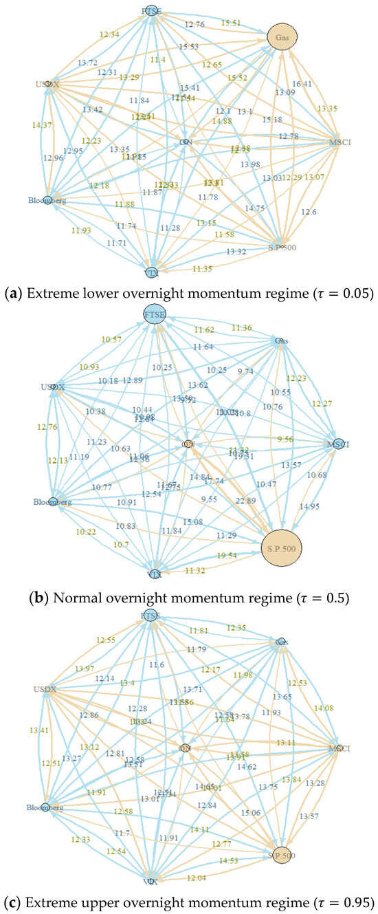
Figure 4.
(a–c) Network connectedness plot (COVID-19). By using pairwise weighting and utilizing colored borders to indicate connectivity, the directional spillover of the system is shown. Khaki nodes denote major transmitters, whereas blue nodes represent receivers. The accompanying statistics show the risk transmitted or received from other markets, and the edge size shows the level of spillover. The interwoven financial environment and the complex web of risk transmission may be better understood with the help of this graphic illustration.
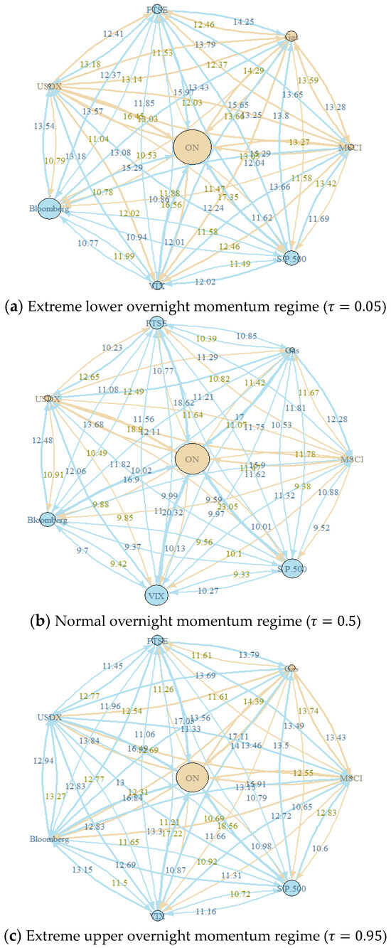
Figure 5.
(a–c) Network connectedness plot (the Russia–Ukraine conflict). By using pairwise weighting and utilizing colored borders to indicate connectivity, the directional spillover of the system is shown. Khaki nodes denote major transmitters, whereas blue nodes represent receivers. The accompanying statistics show the risk transmitted or received from other markets, and the edge size shows the level of spillover. The interwoven financial environment and the complex web of risk transmission may be better understood with the help of this graphic illustration.
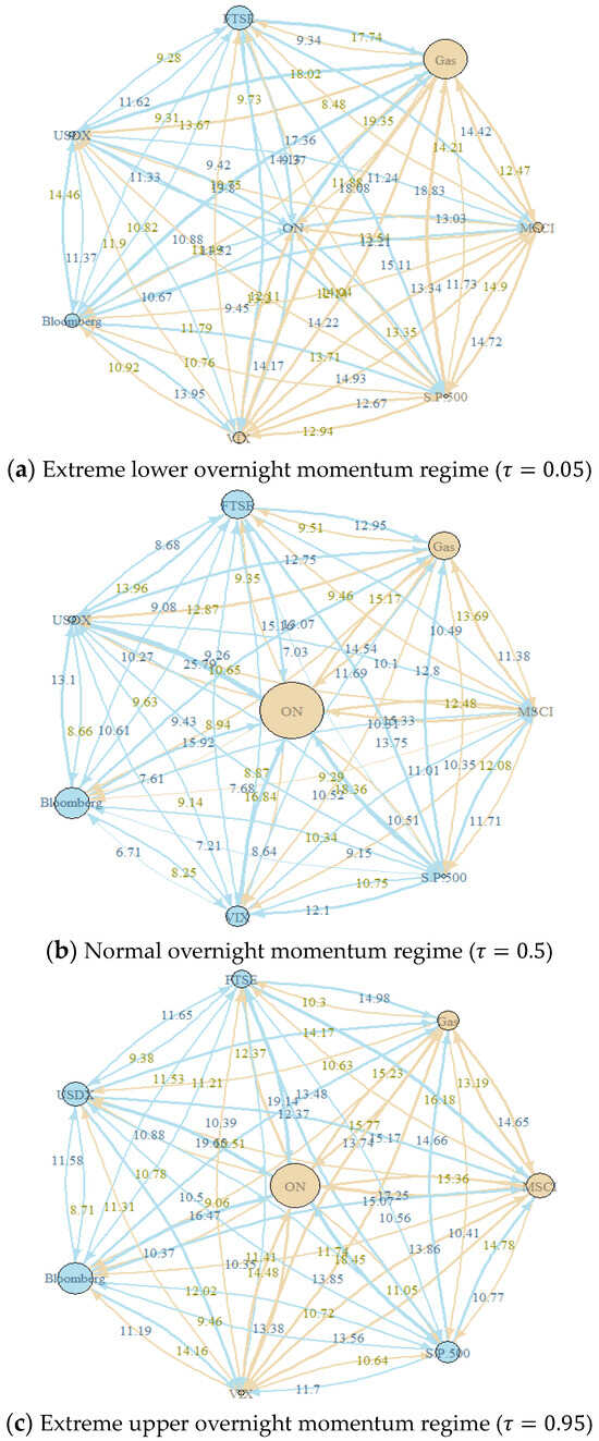
Figure 6.
(a–c) Network connectedness plot (the Israel–Hamas conflict). By using pairwise weighting and utilizing colored borders to indicate connectivity, the directional spillover of the system is shown. Khaki nodes denote major transmitters, whereas blue nodes represent receivers. The accompanying statistics show the risk transmitted or received from other markets, and the edge size shows the level of spillover. The interwoven financial environment and the complex web of risk transmission may be better understood with the help of this graphic illustration.
These findings indicate that investors, politicians, and risk managers might benefit from analyzing overnight momentum in energy markets during crises. Its presence may indicate potential market volatility or the transmission of contagion effects, prompting adjustments in portfolio allocations based on these overnight momentum shifts. To minimize potential losses, one can utilize dynamic hedging techniques or market timing strategies. Authorities may need to adjust their fiscal or monetary policies to maintain financial stability and mitigate systemic risk. Risk forecasts and stress testing scenarios may be enhanced by including overnight momentum in risk assessment models. Changes in overnight momentum may be useful for identifying sector rotation strategies, focusing on businesses with higher resistance to energy market fluctuations during periods of increased volatility.
4.4. The Constancy of Parameters
Two sensitivity studies are conducted to evaluate the sensitivity of the empirical results. In the first practice, we verify this using various rolling-window sizes, specifically 200, 250, and 300 days. The unreported results demonstrate that the spillover pattern remains consistent, regardless of alterations in the rolling window or prediction horizon, indicating that the effects of spillovers between markets are not influenced by these changes. To make sure that the interconnections between the analyzed indices remain constant after making changes to the model and recalculating it, the second technique is to evaluate how extreme quantile selections affect the estimated outcomes. The interconnections between the analyzed indices remain consistent, irrespective of the extreme quantile used.
5. Discussions
This section discusses the results, first highlighting the findings of the static quantile connectedness results for the entire sample and their implications for market conditions. Based on the findings, it is evident that series interactions play a significant role in explaining 85% of the variance in the system. Interestingly, these interactions exhibit an even stronger correlation during periods of market stress. This supports previous research that emphasizes the heightened risk and uncertainty experienced during periods of negative returns. This finding was also reported by Balash and Faizliev (2024), who noted that the primary change in risk distribution may be attributed to the consequences of many unexpected crises on the energy sector. It required a significant amount of time to recover from external shocks (see also Yousaf et al. 2024).
Additionally, the analysis highlights that ON significantly impacts future trading sessions, as it exhibits the highest amount of own-variance spillover. Furthermore, the impact of ON on other network variables is significant, making it a crucial indicator of price fluctuations in interconnected markets. It appears that there are not many options for diversification when faced with challenging market conditions. In addition, the analysis reveals that ON plays a crucial role in transmitting shocks within the system, while VIX is the main entity that receives these shocks. It is evident that the shock transmission of ON reflects the prevailing market sentiment and perception of risk. To fully grasp ON movements, it is crucial to have a thorough comprehension of market microstructure and trading patterns that occur outside of regular trading hours. Liquidity, trade volumes, and market reactions to news must be assessed. The discussion pertains to the reference studies (Hanif et al. 2024; Ustaoglu 2023; Jena et al. 2022) which emphasize the significance of incorporating extreme quantiles and negative return periods to accurately assess the level of interconnection and risk in the market.
Next, utilizing network graphs to visually depict the transmission of shocks and pinpoint the key transmitters and receivers of these shocks within the system, the findings indicate that the overnight momentum in the energy markets has a notable impact on other markets, specifically the S&P 500 and VIX, by transmitting shocks. It is important to recognize the significance of ON in the larger energy market and for policymakers to actively oversee and control it to maintain financial stability. The study also reveals that market connections are more robust during periods of market strain or unpredictability, indicating an increased transmission of disturbances. It is crucial for policymakers to enhance their monitoring and intervention efforts during these periods to mitigate systemic risk. Additionally, the study highlights the significance of considering the dynamics of currency markets and investor behavior when analyzing market connections and formulating appropriate policy responses. Considering the research, it becomes evident that taking proactive policy measures is crucial to enhance market resilience and minimize the effects of contagions.
Finally, we delve into the intricate relationships between financial markets during significant recent crises (the shale oil revolution, COVID-19 pandemic, and ongoing geopolitical conflicts). The results establish that the overnight momentum in oil markets plays a crucial role in shaping the correlation between different factors during these occurrences. These conclusions align with previous studies (e.g., Ziadat et al. 2024; Patel et al. 2024; Umar et al. 2024; Balash and Faizliev 2024). Although these studies do not delve into overnight momentum, they stress the asymmetry spillover between crude oil returns and other stock indices in various market circumstances and show that negative oil returns have a larger influence during bearish periods and a negligible effect during bullish periods. The findings shed new light on the significance of comprehending and efficiently managing risks associated with overnight fluctuations in oil markets amidst periods of economic and geopolitical uncertainty. It is crucial to implement robust policy measures to mitigate risks to global financial markets. This study also indicates that examining the momentum of energy markets overnight during times of crisis can offer valuable insights for investors, politicians, and risk managers in adjusting portfolio allocations and implementing risk management strategies. Additionally, it may be necessary for authorities to adjust fiscal or monetary policies to ensure financial stability and reduce systemic risk.
6. Conclusions and Policy Recommendations
This study explores the transmission mechanism of overnight momentum, a phenomenon triggered by changes in oil prices across various financial markets. It examines the degree of transmission, market conditions, market vulnerability, and fluctuations in connectivity during and after major events. This analysis contributes to a comprehensive understanding of how overnight momentum spreads across the financial sector. Utilizing daily market data from 3 January 2014 to 17 January 2024, we employ the quantile VAR approach to capture nonlinearities, asymmetries, and tail features in financial markets caused by energy shocks.
Our study provides insights into the dynamics of these relationships. We observe that the overnight momentum has the highest level of variance spillover, affecting upcoming trading sessions and triggering price swings in linked markets. Furthermore, this overflow is amplified at extremely high and low quantiles, while a positive overnight momentum reduces the influence. Market stress and volatility facilitate efficient shock transfers during these periods. Understanding these asymmetric dynamics is crucial for developing successful policies and interventions. Thus, the evolution of connectivity during significant political and economic events has been explored, particularly during recent major crises.
This study takes a step further and analyzes how financial markets’ interconnections have changed in response to major global events such as the shale oil revolution, COVID-19 pandemic, Russia–Ukraine war, and Israel–Hamas conflict. Comparable results are revealed, with ON having the largest internal variance spillover among these events.
Additionally, overnight momentum in energy markets plays a crucial role in transmitting shocks to other financial networks such as the S&P 500 and VIX. Systemic importance is essential for maintaining financial stability. The stability of the energy market is a concern that policymakers need to keep an eye on and take steps to protect against. The need for taking proactive measures to enhance market resilience is highlighted by the rapid growth of online trading (ON). Whenever there is market stress or volatility, shocks are transmitted more easily due to the interconnection of the markets. Financial market stability and reduction in systemic risk can be achieved by increased government intervention and monitoring.
Overall, this study strengthens the importance of recognizing and managing the risks associated with overnight changes in the oil market, especially during periods of economic and geopolitical uncertainty. It suggests that strong government actions are needed to address these risks. Additionally, understanding the overnight momentum of the energy market can help stakeholders such as politicians, investors, and risk managers make informed decisions and take preventive measures to mitigate risk during crises. This study also provides policy implications, including the need for policymakers to proactively implement measures to enhance market stability and mitigate systemic risk during periods of market volatility. Monitoring and controlling overnight momentum is crucial for ensuring financial stability, and policymakers should prioritize this during times of market strain or unpredictability. Considering currency markets and investor behavior is important for developing policy responses that enhance market resilience and mitigate contagion effects. Policymakers should also address potential dangers associated with sudden shifts in oil markets, particularly during periods of economic and geopolitical instability. Examining overnight momentum in energy markets during crises can provide valuable insights for investors, politicians, and risk managers, informing decisions on portfolio allocations and risk management strategies. Adjustments to fiscal or monetary policies may be necessary to maintain financial stability and reduce systemic risk.
Funding
This research received no external funding.
Informed Consent Statement
Not applicable.
Data Availability Statement
The data that support the findings of this study are available from the author upon reasonable request.
Conflicts of Interest
The authors declare no conflict of interest.
Abbreviations
| QVAR | quantile-based vector autoregression |
| GFEVD | generalized forecast error variance decomposition |
| TCI | total connectedness index |
| JB | Jarque–Bera |
| BIC | Bayesian information criterion |
| ON | overnight momentum in oil markets |
| MSCI | Morgan Stanley Capital International World Stock Index |
| Gas | S&P GSCI Natural Gas |
| FTSE | Financial Times Stock Exchange Index |
| USDX | US Dollar Index |
| Bloomberg | Bloomberg Commodities Index |
| S&P.500 | S&P 500 Index |
| VIX | Volatility Index |
| JB | Jarque and Bera |
| ERS | Elliott, Rothenberg, and Stock |
References
- Abakah, Emmanuel Joel Aikins, Aviral Kumar Tiwari, Imhotep Paul Alagidede, and Luis Alberiko Gil-Alana. 2022. Re-examination of risk-return dynamics in international equity markets and the role of policy uncertainty, geopolitical risk and VIX: Evidence using Markov-switching copulas. Finance Research Letters 47: 102535. [Google Scholar] [CrossRef]
- Adams, Zeno, Solène Collot, and Maria Kartsakli. 2020. Have commodities become a financial asset? Evidence from ten years of Financialization. Energy Economics 89: 104769. [Google Scholar] [CrossRef]
- Ahmed, Abdullahi D., and Rui Huo. 2020. Volatility transmissions across international oil market, commodity futures and stock markets: Empirical evidence from China. Energy Economics 93: 104741. [Google Scholar] [CrossRef]
- Alola, Andrew Adewale. 2021. Evidence of speculative bubbles and regime switch in real estate market and crude oil price: Insight from Saudi Arabia. International Journal of Finance & Economics 26: 3473–83. [Google Scholar]
- Al-Yahyaee, Khamis Hamed, Walid Mensi, Ahmet Sensoy, and Sang Hoon Kang. 2019. Energy, precious metals, and GCC stock markets: Is there any risk spillover? Pacific-Basin Finance Journal 56: 45–70. [Google Scholar] [CrossRef]
- Ando, Tomohiro, Matthew Greenwood-Nimmo, and Yongcheol Shin. 2022. Quantile connectedness: Modeling tail behavior in the topology of financial networks. Management Science 68: 2401–31. [Google Scholar] [CrossRef]
- Anscombe, Francis J., and William J. Glynn. 1983. Distribution of the kurtosis statistic b 2 for normal samples. Biometrika 70: 227–34. [Google Scholar] [CrossRef]
- Appiah, Michael Karikari, Elikplim Ameko, Theodora Akweley Asiamah, and Rahmat Quaigrane Duker. 2023. Blue economy investment and sustainability of Ghana’s territorial waters: An application of structural equation modelling. International Journal of Sustainable Engineering, 1–15. [Google Scholar] [CrossRef]
- Appiah-Konadu, Paul, Nathaniel Amoah, and Mina Afia Acquah. 2022. Sustainable Investment in Africa: Beyond ESG. In Management and Leadership for a Sustainable Africa, Volume 1: Dimensions, Practices and Footprints. Cham: Springer International Publishing, pp. 273–288. [Google Scholar]
- Balash, Vladimir, and Alexey Faizliev. 2024. Volatility spillovers across Russian oil and gas sector. Evidence of the impact of global markets and extraordinary events. Energy Economics 129: 107202. [Google Scholar] [CrossRef]
- Batten, Jonathan A., Harald Kinateder, Peter G. Szilagyi, and Niklas F. Wagner. 2021. Hedging stocks with oil. Energy Economics 93: 104422. [Google Scholar] [CrossRef]
- Baumöhl, Eduard, and Syed Jawad Hussain Shahzad. 2019. Quantile coherency networks of international stock markets. Finance Research Letters 31: 119–29. [Google Scholar] [CrossRef]
- Bogousslavsky, Vincent. 2021. The cross-section of intraday and overnight returns. Journal of Financial Economics 141: 172–94. [Google Scholar] [CrossRef]
- Cecchetti, Stephen G., and Lianfa Li. 2008. Do capital adequacy requirements matter for monetary policy? Economic Inquiry 46: 643–59. [Google Scholar] [CrossRef]
- Chatziantoniou, Ioannis, Ahmed H. Elsayed, David Gabauer, and Giray Gozgor. 2023. Oil price shocks and exchange rate dynamics: Evidence from decomposed and partial connectedness measures for oil importing and exporting economies. Energy Economics 120: 106627. [Google Scholar] [CrossRef]
- d’Agostino, Ralph B. 1971. An omnibus test of normality for moderate and large size samples. Biometrika 58: 341–48. [Google Scholar] [CrossRef]
- Daskalaki, Charoula, and George Skiadopoulos. 2011. Should investors include commodities in their portfolios after all? New evidence. Journal of Banking & Finance 35: 2606–26. [Google Scholar]
- Demirer, Rıza, Roman Ferrer, and Syed Jawad Hussain Shahzad. 2020. Oil price shocks, global financial markets and their connectedness. Energy Economics 88: 104771. [Google Scholar] [CrossRef]
- Diebold, Francis X., and Kamil Yilmaz. 2012. Better to give than to receive: Predictive directional measurement of volatility spillovers. International Journal of Forecasting 28: 57–66. [Google Scholar] [CrossRef]
- Elliott, Graham, Thomas J. Rothenberg, and James H. Stock. 1996. Efficient Tests for an Autoregressive Unit Root. Econometrica 64: 813–36. [Google Scholar] [CrossRef]
- Ewing, Bradley T., and Farooq Malik. 2016. Volatility spillovers between oil prices and the stock market under structural breaks. Global Finance Journal 29: 12–23. [Google Scholar] [CrossRef]
- Farid, Saqib, Ghulam Mujtaba Kayani, Muhammad Abubakr Naeem, and Syed Jawad Hussain Shahzad. 2021. Intraday volatility transmission among precious metals, energy and stocks during the COVID-19 pandemic. Resources Policy 72: 102101. [Google Scholar] [CrossRef]
- Farid, Saqib, Muhammad Abubakr Naeem, Andrea Paltrinieri, and Rabindra Nepal. 2022. Impact of COVID-19 on the quantile connectedness between energy, metals and agriculture commodities. Energy Economics 109: 105962. [Google Scholar] [CrossRef] [PubMed]
- Fasanya, Ismail O., Oluwasegun B. Adekoya, and Abiodun M. Adetokunbo. 2021. On the connection between oil and global foreign exchange markets: The role of economic policy uncertainty. Resources Policy 72: 102110. [Google Scholar] [CrossRef]
- Fisher, Thomas J., and Colin M. Gallagher. 2012. New weighted portmanteau statistics for time series goodness of fit testing. Journal of the American Statistical Association 107: 777–87. [Google Scholar] [CrossRef]
- Goodell, John W. 2020. COVID-19 and finance: Agendas for future research. Finance Research Letters 35: 101512. [Google Scholar] [CrossRef] [PubMed]
- Griffin, John M., Xiuqing Ji, and J. Spencer Martin. 2003. Momentum investing and business cycle risk: Evidence from pole to pole. The Journal of Finance 58: 2515–47. [Google Scholar] [CrossRef]
- Grinblatt, Mark, Sheridan Titman, and Russ Wermers. 1995. Momentum investment strategies, portfolio performance, and herding: A study of mutual fund behavior. American Economic Review 85: 1088–105. [Google Scholar]
- Guhathakurta, Kousik, Saumya Ranjan Dash, and Debasish Maitra. 2020. Period specific volatility spillover based connectedness between oil and other commodity prices and their portfolio implications. Energy Economics 85: 104566. [Google Scholar] [CrossRef]
- Gunay, Samet, and Bekir Emre Kurtulmuş. 2021. COVID-19 social distancing and the US service sector: What do we learn? Research in International Business and Finance 56: 101361. [Google Scholar] [CrossRef]
- Hanif, Asma, A. I. K. Butt, Shabir Ahmad, Rahim Ud Din, and Mustafa Inc. 2021. A new fuzzy fractional order model of transmission of Covid-19 with quarantine class. The European Physical Journal Plus 136: 1–28. [Google Scholar] [CrossRef]
- Hanif, Waqas, Sinda Hadhri, and Rim El Khoury. 2024. Quantile spillovers and connectedness between oil shocks and stock markets of the largest oil producers and consumers. Journal of Commodity Markets 34: 100404. [Google Scholar] [CrossRef]
- Huang, Alex YiHou, Ming-Che Hu, and Quang Thai Truong. 2021. Asymmetrical impacts from overnight returns on stock returns. Review of Quantitative Finance and Accounting 56: 849–89. [Google Scholar] [CrossRef]
- Hung, Ngo Thai. 2021. Oil prices and agricultural commodity markets: Evidence from pre and during COVID-19 outbreak. Resources Policy 73: 102236. [Google Scholar] [CrossRef]
- Hussain, Muntazir, Gilney Figueira Zebende, Usman Bashir, and Ding Donghong. 2017. Oil price and exchange rate co-movements in Asian countries: Detrended cross-correlation approach. Physica A: Statistical Mechanics and its Applications 465: 338–46. [Google Scholar] [CrossRef]
- Jarque, Carlos M., and Anil K. Bera. 1980. Efficient tests for normality, homoscedasticity and serial independence of regression residuals. Economics Letters 6: 255–59. [Google Scholar] [CrossRef]
- Jebabli, Ikram, Noureddine Kouaissah, and Mohamed Arouri. 2022. Volatility spillovers between stock and energy markets during crises: A comparative assessment between the 2008 global financial crisis and the COVID-19 pandemic crisis. Finance Research Letters 46: 102363. [Google Scholar] [CrossRef]
- Jegadeesh, Narasimhan, and Sheridan Titman. 2002. Cross-sectional and time-series determinants of momentum returns. The Review of Financial Studies 15: 143–57. [Google Scholar] [CrossRef]
- Jena, Sangram Keshari, Aviral Kumar Tiwari, Emmanuel Joel Aikins Abakah, and Shawkat Hammoudeh. 2022. The connectedness in the world petroleum futures markets using a quantile VAR approach. Journal of Commodity Markets 27: 100222. [Google Scholar] [CrossRef]
- Jensen, Gerald R., Robert R. Johnson, and Jeffrey M. Mercer. 2000. Efficient use of commodity futures in diversified portfolios. Journal of Futures Markets: Futures, Options, and Other Derivative Products 20: 489–506. [Google Scholar] [CrossRef]
- Ji, Qiang, Bing-Yue Liu, and Ying Fan. 2019. Risk dependence of CoVaR and structural change between oil prices and exchange rates: A time-varying copula model. Energy Economics 77: 80–92. [Google Scholar] [CrossRef]
- Jiang, Zhuhua, and Seong-Min Yoon. 2020. Dynamic co-movement between oil and stock markets in oil-importing and oil-exporting countries: Two types of wavelet analysis. Energy Economics 90: 104835. [Google Scholar] [CrossRef]
- Karim, Sitara, Muhammad Abubakr Naeem, Min Hu, Dayong Zhang, and Farhad Taghizadeh–Hesary. 2022a. Determining dependence, centrality, and dynamic networks between green bonds and financial markets. Journal of Environmental Management 318: 115618. [Google Scholar] [CrossRef] [PubMed]
- Karim, Sitara, Shabeer Khan, Nawazish Mirza, Suha M. Alawi, and Farhad Taghizadeh-Hesary. 2022b. Climate finance in the wake of COVID-19: Connectedness of clean energy with conventional energy and regional stock markets. Climate Change Economics 13: 2240008. [Google Scholar] [CrossRef]
- Koenker, Roger, and Gilbert Bassett, Jr. 1978. Regression Quantiles. Econometrica: Journal of the Econometric Society, 33–50. [Google Scholar] [CrossRef]
- Koop, Gary, M. Hashem Pesaran, and Simon M. Potter. 1996. Impulse response analysis in nonlinear multivariate models. Journal of Econometrics 74: 119–47. [Google Scholar] [CrossRef]
- Lin, Boqiang, and Tong Su. 2020a. Mapping the oil price-stock market nexus researches: A scientometric review. International Review of Economics & Finance 67: 133–47. [Google Scholar]
- Lin, Boqiang, and Tong Su. 2020b. The linkages between oil market uncertainty and Islamic stock markets: Evidence from quantile-on-quantile approach. Energy Economics 88: 104759. [Google Scholar] [CrossRef]
- Liu, Fang, Muhammad Umair, and Junjun Gao. 2023a. Assessing oil price volatility co-movement with stock market volatility through quantile regression approach. Resources Policy 81: 103375. [Google Scholar] [CrossRef]
- Liu, Zhenya, Shanglin Lu, Bo Li, and Shixuan Wang. 2023b. Time series momentum and reversal: Intraday information from realized semivariance. Journal of Empirical Finance 72: 54–77. [Google Scholar] [CrossRef]
- Lou, Dong, Christopher Polk, and Spyros Skouras. 2019. A tug of war: Overnight versus intraday expected returns. Journal of Financial Economics 134: 192–213. [Google Scholar] [CrossRef]
- Luo, Jiawen, Hardik A. Marfatia, Qiang Ji, and Tony Klein. 2023. Co-volatility and asymmetric transmission of risks between the global oil and China’s futures markets. Energy Economics 117: 106466. [Google Scholar] [CrossRef]
- Mensi, Walid, Makram Beljid, Adel Boubaker, and Shunsuke Managi. 2013. Correlations and volatility spillovers across commodity and stock markets: Linking energies, food, and gold. Economic Modelling 32: 15–22. [Google Scholar] [CrossRef]
- Mensi, Walid, Mobeen Ur Rehman, and Xuan Vinh Vo. 2021. Dynamic frequency relationships and volatility spillovers in natural gas, crude oil, gas oil, gasoline, and heating oil markets: Implications for portfolio management. Resources Policy 73: 102172. [Google Scholar] [CrossRef]
- Mensi, Walid, Juan C. Reboredo, Andrea Ugolini, and Xuan Vinh Vo. 2022. Switching connectedness between real estate investment trusts, oil, and gold markets. Finance Research Letters 49: 103112. [Google Scholar] [CrossRef]
- Ming, Lei, Wuqi Song, and Minyi Dong. 2023. Revisiting time series momentum in China’s commodity futures market: Evidence on sources of momentum profits. Economic Modelling 128: 106522. [Google Scholar] [CrossRef]
- Naeem, Muhammad Abubakr, and Sitara Karim. 2021. Tail dependence between bitcoin and green financial assets. Economics Letters 208: 110068. [Google Scholar] [CrossRef]
- Naeem, Muhammad Abubakr, Raazia Gul, Muhammad Shafiullah, Sitara Karim, and Brian M. Lucey. 2023a. Tail risk spillovers between Shanghai oil and other markets. Energy Economics 130: 107182. [Google Scholar] [CrossRef]
- Naeem, Muhammad Abubakr, Thi Thu Ha Nguyen, Sitara Karim, and Brian M. Lucey. 2023b. Extreme downside risk transmission between green cryptocurrencies and energy markets: The diversification benefits. Finance Research Letters 58: 104263. [Google Scholar] [CrossRef]
- Naeem, Muhammad Abubakr, Raazia Gul, Ahmet Faruk Aysan, and Umar Nawaz Kayani. 2024. Oil shocks and the transmission of higher-moment information in US industry: Evidence from an asymmetric puzzle. Borsa Istanbul Review. [Google Scholar] [CrossRef]
- Nazlioglu, Saban, N. Alper Gormus, and Uğur Soytas. 2016. Oil prices and real estate investment trusts (REITs): Gradual-shift causality and volatility transmission analysis. Energy Economics 60: 168–75. [Google Scholar] [CrossRef]
- Nazlioglu, Saban, Rangan Gupta, Alper Gormus, and Ugur Soytas. 2020. Price and volatility linkages between international REITs and oil markets. Energy Economics 88: 104779. [Google Scholar] [CrossRef]
- Patel, Ritesh, Mariya Gubareva, and Muhammad Zubair Chishti. 2024. Assessing the connectedness between cryptocurrency environment attention index and green cryptos, energy cryptos, and green financial assets. Research in International Business and Finance 70: 102339. [Google Scholar] [CrossRef]
- Pesaran, H. Hashem, and Yongcheol Shin. 1998. Generalized impulse response analysis in linear multivariate models. Economics Letters 58: 17–29. [Google Scholar] [CrossRef]
- Sensoy, Ahmet, Erk Hacihasanoglu, and Duc Khuong Nguyen. 2015. Dynamic convergence of commodity futures: Not all types of commodities are alike. Resources Policy 44: 150–60. [Google Scholar] [CrossRef]
- Silvennoinen, Annastiina, and Susan Thorp. 2013. Financialization, crisis and commodity correlation dynamics. Journal of International Financial Markets, Institutions and Money 24: 42–65. [Google Scholar] [CrossRef]
- Topcu, Mert, and Omer Serkan Gulal. 2020. The impact of COVID-19 on emerging stock markets. Finance Research Letters 36: 101691. [Google Scholar] [CrossRef]
- Umar, Zaghum, Nader Trabelsi, and Adam Zaremba. 2021. Oil shocks and equity markets: The case of GCC and BRICS economies. Energy Economics 96: 105155. [Google Scholar] [CrossRef]
- Umar, Zaghum, Sinda Hadhri, Emmanuel Joel Aikins Abakah, Muhammad Usman, and Muhammad Umar. 2024. Return and volatility spillovers among oil price shocks and international green bond markets. Research in International Business and Finance 69: 102254. [Google Scholar] [CrossRef]
- Ustaoglu, Erkan. 2023. Extreme return connectedness between renewable energy tokens and renewable energy stock markets: Evidence from a quantile-based analysis. Environmental Science and Pollution Research 31: 5086–99. [Google Scholar] [CrossRef]
- Wei, Yu, Yaojie Zhang, and Yudong Wang. 2022. Information connectedness of international crude oil futures: Evidence from SC, WTI, and Brent. International Review of Financial Analysis 81: 102100. [Google Scholar] [CrossRef]
- Wen, Xiaoqian, Yu Wei, and Dengshi Huang. 2012. Measuring contagion between energy market and stock market during financial crisis: A copula approach. Energy Economics 34: 1435–46. [Google Scholar] [CrossRef]
- Wen, Zhuzhu, Xu Gong, Diandian Ma, and Yahua Xu. 2021. Intraday momentum and return predictability: Evidence from the crude oil market. Economic Modelling 95: 374–84. [Google Scholar] [CrossRef]
- Yang, Tianle, Fangxing Zhou, Min Du, Qunyang Du, and Shirong Zhou. 2023. Fluctuation in the global oil market, stock market volatility, and economic policy uncertainty: A study of the US and China. The Quarterly Review of Economics and Finance 87: 377–87. [Google Scholar] [CrossRef]
- Yousaf, Imran, Muhammad Shahzad Ijaz, Muhammad Umar, and Yanshuang Li. 2024. Exploring volatility interconnections between AI tokens, AI stocks, and fossil fuel markets: Evidence from time and frequency-based connectedness analysis. Energy Economics 133: 107490. [Google Scholar] [CrossRef]
- Zhou, Min, and Xiaoqun Liu. 2022. Overnight-intraday mispricing of Chinese energy stocks: A view from financial anomalies. Front. Energy Res. 9: 807881. [Google Scholar] [CrossRef]
- Ziadat, Salem Adel, Walid Mensi, and Sang Hoon Kang. 2024. Frequency spillovers between oil shocks and stock markets of top oil-producing and-consuming economies. Energy 291: 130239. [Google Scholar] [CrossRef]
- Zorgati, Mouna Ben Saad. 2023. Risk Measure between exchange rate and oil price during crises: Evidence from oil-importing and oil-exporting countries. Journal of Risk and Financial Management 16: 250. [Google Scholar] [CrossRef]
Disclaimer/Publisher’s Note: The statements, opinions and data contained in all publications are solely those of the individual author(s) and contributor(s) and not of MDPI and/or the editor(s). MDPI and/or the editor(s) disclaim responsibility for any injury to people or property resulting from any ideas, methods, instructions or products referred to in the content. |
© 2024 by the author. Licensee MDPI, Basel, Switzerland. This article is an open access article distributed under the terms and conditions of the Creative Commons Attribution (CC BY) license (https://creativecommons.org/licenses/by/4.0/).

