Constant Leverage Covering Strategy for Equity Momentum Portfolio with Transaction Costs

Abstract

The Constant Leverage covering strategy for the equity momentum portfolio (CLvg) developed in this project cannot mask its shortcomings by increasing leverage. It has to successfully forecast and avoid more losses than profits to perform better than the momentum portfolio. This approach is different from other covering strategies available in the literature that focus on increasing the right tail of the momentum returns distribution at a faster rate than they increase the left tail. The CLvg strategy only depends on past information and uses the daily volatility of the loser portfolio to determine episodes of high and low volatility. The daily volatility of the loser portfolio has a stronger relationship with large negative momentum returns than the daily volatility of the momentum portfolio. The daily volatility of the loser portfolio also has a weaker relationship with larger positive monthly returns, and it is more predictable because it has a higher volatility persistence. The negative effects of transaction costs on the CLvg strategy are measured using bid and ask prices reported by CRSP from 1992 to 2021. During this period, the stock market presented an average excess return of 9.19% and a Sharpe ratio of 0.61, and 9.74% of its returns were crashes, which is a better performance than the momentum portfolio. The CLvg adjusted by transaction costs presented excess returns of 16.93% and a Sharpe ratio of 0.84, and only 8.31% of its returns were crashes.

1. Introduction

The momentum portfolio is a market anomaly because it outperforms the market using information stored in past monthly returns. Jegadeesh and Titman (1993) show that, if stocks are ranked by their past returns, the worst past performers will also underperform the following month (loser portfolio) and the best past performers will also overperform the following month (winner portfolio). The momentum portfolio is formed by buying the winner portfolio and selling the loser portfolio (WmL).

The literature has developed several covering strategies to minimize the main problem of the momentum portfolio: the existence of crashes (monthly losses larger than −5%), as documented by Barroso and Santa-Clara (2015). The problem of the available covering strategies for the momentum portfolio is that they depend on past information. Grundy and Martin (2001) use forward-looking information. Barroso and Santa-Clara (2015) and Daniel and Moskowitz (2016) minimize the use of forward-looking data, but their covering strategies still depend on the in-sample average volatility of the stock market, which is problematic because practitioners should know this value before they implement the covering strategies.

This project identifies a U-shaped relationship between the volatility of the loser portfolio and momentum returns and uses it to construct a covering strategy for the momentum portfolio that only depends on past information. This strategy also accounts for transaction costs, which makes it implementable by practitioners.

The development of a Constant Leverage (CLvg) covering strategy avoids exploiting the returns distributions of the momentum portfolio in a way that is unpalatable for practitioners: increasing the average return by increasing the right tail of the distribution at a faster rate than increasing the left tail of the distribution. The covering strategy of the CLvg is different from the Constant Volatility (CVol) strategy proposed by Barroso and Santa-Clara (2015). The CVol strategy focuses on increasing future returns when the expected volatility of the momentum portfolio is low. This turns mild positive returns into large positive returns, but it also transforms mild negative returns into large negative returns.

The CLvg strategy has higher expected returns and smaller standard deviations, and it minimizes the presence of crashes when compared against the stock market, the momentum portfolio, and the CVol covering strategy. This project uses the bid and ask prices reported by the CRSP from 1992 to 2021 to compute transaction costs at the individual stock level. During this period, the stock market presented an average excess return of 9.19% and a Sharpe ratio of 0.61, and 9.74% of the stock market’s returns were crashes. The WmL portfolio adjusted by transaction costs presented excess returns of 10.99% and a Sharpe ratio of 0.31, and 18.05% of the momentum portfolio’s returns were crashes. The CLvg covering strategy adjusted by transaction costs presented excess returns of 16.93% and a Sharpe ratio of 0.84, and only 8.31% of its returns were crashes.

Section 5 shows how to use the symmetrical U-shaped relationship between momentum returns volatility and momentum returns to explain the weaknesses of the CVol. The CVol buys multiple momentum portfolios in episodes of low volatility to compensate for cutting extremely positive returns during episodes of high volatility. However, this increase in leverage causes a second problem: It turns mild negative returns associated with low volatility into large negative returns.

The CVol strategy exploits the positive average of the momentum returns distributions to mask its shortcomings (the trough of the U-shaped relationship between momentum returns volatility and momentum returns lies to the right of zero percent, as discussed in Section 5. However, the introduction of transaction costs significantly reduces the positive effects of increasing leverage and reduces the profitability of the CVol.

2. Literature Review: Momentum Everywhere

The momentum literature is mostly a collection of empirical findings. Singh and Walia (2020) explain that there is no unified theoretical framework that explains momentum. Instead, there are two leading theories. Some researchers explain the excess returns of momentum as a compensation for risk: Conrad and Kaul (1998), Moskowitz and Grinblatt (1999), Li (2017), and Ruenzi and Weigert (2018). Other research explains the excess returns of momentum using behavioral finance: Barberis et al. (1998), Vayanos and Woolley (2013), Booth et al. (2016), Chen and Lu (2017), and Hur and Singh (2019).

Momentum returns are not constrained to the American stock market. Rouwenhorst (1998) finds positive momentum returns in international assets. Chan et al. (2000) document profitable momentum strategies on international stock market indices. Jostova et al. (2013) record significant momentum returns for noninvestment-grade corporate bonds. Gorton et al. (2012) find momentum returns in commodity markets. Finally, Okunev and White (2003) note momentum in currency markets.

However, the momentum portfolio has two shortcomings. The first weakness is the negative effects of transaction costs. The momentum portfolio has a lower Sharpe ratio than the stock market after considering transaction costs. Lesmond et al. (2004) estimate transaction costs for the momentum strategy and argue that the momentum portfolio will not be profitable under transaction costs. Korajczyk and Sadka (2004) find similar results.

The second shortcoming is the existence of large and frequent crashes. Investors with standard risk aversion should not be interested in the momentum portfolio, because it presents frequent crashes that offset the appeal of a high Sharpe ratio. Crashes plague the momentum portfolio even if transaction costs are ignored. Between 1927 and 2021, the largest monthly loss of the momentum portfolio was −77.46% in August 1932. Meanwhile, the largest monthly loss of the stock market was −29.21% in September 1939. Crashes represent 10.9% of the stock market returns but 12.6% of the momentum portfolio returns. Investors might not be interested in the momentum portfolio because it takes years to recover from one crash.

Literature Review: Covering Strategies with Forward-Looking Biases and Volatility

Cujean and Hasler (2017) reported that there are narrowly defined points in time when equity returns become predictable: after a major sell-off during a financial crisis, most equities bounce back aggressively as there is a fast adjustment between current depressed prices and more optimistic expectations.

Barroso and Santa-Clara (2015) documented that this predictability of a widespread rebound in asset prices creates large losses from selling the loser portfolio, and it tends to occur after periods of high volatility. Understanding the relationship between volatility and momentum portfolio underperformance rekindled academic interest. The following researchers have identified a strong relationship between the momentum portfolio performance and volatility: Wang and Xu (2015), Fan et al. (2018), Lim et al. (2018), and Demirer and Zhang (2019).

The first generation of covering strategies for the momentum portfolio has a forward-looking bias. Grundy and Martin (2001) develop the first covering strategy for the momentum portfolio. Their insight is that the beta of the momentum portfolio is a useful signal of future crashes because it takes negative values after the momentum portfolio presents crashes. During an upside stock market, the winner portfolio tends to have high beta stocks while the loser portfolio tends to have low beta stocks. However, if the stock market falls during the formation period, the loser portfolio will tend to have the high beta stocks that fall in tandem with the market, while the winner portfolio will have low beta stocks. Therefore, when the market rebounds, the momentum portfolio crashes because it has a net negative beta. Unfortunately, they estimate dynamic betas using the whole sample. They assess the profitability of the beta-hedged portfolio based on in-sample beta estimates. However, practitioners may not reach the same level of profitability with out-of-sample beta estimates.

The second generation of covering strategies identifies a signal that uses only past information to forecast crashes. Barroso and Santa-Clara (2015) document that episodes of high daily returns volatility in the momentum portfolio occur at the same time as large negative monthly returns in the momentum. They document that episodes of high volatility are forecastable because the daily returns volatility of the momentum portfolio has a high volatility persistence. Section 5 shows that this is a successful signal because the daily returns volatility of the momentum portfolio has a symmetrical U-shaped relationship with monthly returns of the momentum portfolio. Using episodes of high volatility to reduce leverage and cut future monthly returns will reduce crashes but will also reduce large positive monthly returns. This negative effect is not discussed by Barroso and Santa-Clara (2015). Furthermore, the negative effects of cutting leverage are masked by the positive effects of increasing leverage.

However, the second generation of covering strategies for the momentum portfolio adjusts the volatility with a forward-looking bias. Barroso and Santa-Clara (2015) input an ad hoc volatility target of 12% after observing the whole sample and without discussing the negative effects of increasing or decreasing this target. Daniel and Moskowitz (2016) use the same signal, but they adjust the volatility to be equal to the in-sample average volatility of the stock market. Also, they do not discuss negative effects of a larger or smaller volatility target. This is problematic because practitioners should know which volatility target to select at the time of implementation.

The negative effects of a forward-looking target are even more concerning when the covering strategy consists of increasing and decreasing leverage. The Constant Volatility covering strategy (CVol) (Barroso and Santa-Clara 2015) and the Dynamic Volatility covering strategy (Daniel and Moskowitz 2016) consist of the same relationship between signal and target: increasing leverage (buy multiple momentum portfolios) when the signal is below the target and decreasing leverage (buy a fraction of the momentum portfolio) when the signal is above the target. The daily returns volatility of the momentum portfolio is highly persistent, but it is not always successful at predicting crashes.

Covering strategies for the momentum portfolio focus on forecasting and avoiding crashes using information stored in past daily returns. This is remarkable because the momentum portfolio already outperforms the stock market by using information stored in monthly returns that had been publicly known for more than twelve months.

3. Contribution: Covering Strategies without Forward-Looking Biases

The main contribution of this project is the development of a covering strategy for the momentum portfolio that is implementable by practitioners because it only depends on past information. The Constant Leverage covering strategy (CLvg) is more profitable than the stock market even after accounting for transaction costs. This project compares the CLvg against the CVol strategy developed by Barroso and Santa-Clara (2015) under transaction costs. The CVol focuses on increasing the average return of the momentum portfolio while increasing negative returns that are related to highly persistent volatility. The CLvg focuses on avoiding extremely high returns and crashes that can be forecasted because they are related to highly persistent volatility.

The CLvg developed in this project lacks a compensation mechanism to mask its shortcomings. The CLvg buys the momentum portfolio when the signal is below the target, and it buys one month of treasury bills when the signal is above the target. Therefore, the CLvg can only have a better performance than the momentum portfolio if it successfully forecasts and avoids more negative monthly returns than positive monthly returns.

The CLvg uses the daily returns volatility of the loser portfolio as a signal because the largest crashes in the momentum portfolio come from selling the loser portfolio and not from buying the winner portfolio. Additionally, the volatility persistence of the loser portfolio is even higher than the volatility of the momentum portfolio, which increases the accuracy of the volatility forecasts. This paper documents a U-shaped relationship between daily loser portfolio returns volatility and monthly momentum returns that leans to the left. High daily volatility in the loser portfolio has a stronger relationship with large negative monthly losses in the momentum portfolio than with large monthly profits.

This project develops a methodology to select the volatility targets using only past information. It constructs an optimization grid that has multiple volatility targets. The volatility target for the next month is equal to the volatility target that maximized the Sharpe ratio over the past ten years. The ten-year window is updated every month.

The CLvg covering strategy does not improve the performance of the momentum portfolio by predicting the future, but by avoiding the empirically regular momentum portfolio crashes that are predictable and related to periods of high volatility in the loser portfolio. The momentum portfolio presents unpredictable, large losses from holding the winner portfolio when a large negative shock hits the whole stock market. However, the stock market tends to process the unpredictable shocks in the same way, making some momentum portfolio crashes predictable, as shown in Section 5. The arrival of the negative shock increases the returns volatility of all stocks, but the increases in volatility are more acute in the stocks that form the loser portfolio. The high-volatility episodes in the loser portfolio start when the large negative shock arrives and end after the large negative shock dissipates. Momentum portfolio crashes that occur when the sell-off ends can be avoided by not holding the momentum portfolio during episodes of high volatility in the loser portfolio (even when no one knows when the high volatility in the loser portfolio will end).

The high retention rates of the winner and loser portfolios mitigate the negative effects of transaction costs. Section 4.1 shows that the momentum portfolio becomes unprofitable under transaction costs if the turnover rate is one hundred percent: the expected excess return falls from 17.99% to −4.38%. However, not all shares enter and leave the winner and loser portfolios each month. About 55% of the shares in the loser and winner portfolios do not pay transaction costs in a given month, because they remain in the same portfolio the following month. About 35% of the shares pay only half of the transaction cost because they enter or leave the portfolio in the same month. Only about 10% of the shares enter and leave the winner and loser portfolios in the same month and pay the full transaction costs. After adjusting transaction costs for actual turnover, momentum portfolios have an average excess return of 10.99%, which is higher than the 9.19% of the stock market.

The CLvg has a higher expected return and Sharpe ratio than the CVol, the momentum portfolio, and the stock market even after considering transaction costs adjusted by turnover. This project uses closing bid and ask prices reported by the Center for Research in Security Prices (CRSP) from 1992 to 2021 to compute transaction costs at the individual stock level. In this period, the stock market presented an average excess return of 9.19% and a Sharpe ratio of 0.61, and 9.74% of its returns were crashes. The momentum portfolio presented excess returns of 10.99% and a Sharpe ratio of 0.31, and 18.05% of its returns were crashes. The CVol presented an average excess return of 16.58% and a Sharpe ratio of 0.55, and 18.65% of its returns were crashes. The CLvg presented excess returns of 16.93% and a Sharpe ratio of 0.84, and only 8.31% of its returns were crashes.

3.1. Methodology: Individual Stock Returns with Transaction Costs

This project reproduces the quoted spread estimate used by Bhardwaj and Brooks (1992) and Lesmond et al. (2004) to measure transaction costs. Returns with transaction costs are equal to the individual stock returns with dividends adjusted by the price spread at the closing price, as shown in Equation (1), where $r_{i,t}^{cost}$ is the individual stock price return plus the dividend return adjusted by transaction costs assuming that the stock is bought and sold in the same period t. $P_{i,t-1}$ is the share price in the previous period. $P_{i,t}$ is the share price in the current period, $f_{i,t}$ is a price adjustment factor that the CRSP uses to correct for splits or new stock issues, and $d_{i,t}$ is the dividend return that the stock receives at time t. $P_{i,t}^{ask}$ and $P_{i,t}^{bid}$ are the last representative ask and bid prices before the market closes at trading day t.

Equation (1). Stock returns including transaction cost for a round trip.

$$r_{i,t}^{cost}=\left(\frac{P_{i,t}\ast f_{i,t}+d_{i,t}}{P_{i,t-1}}-1\right)-\left(\frac{P_{i,t}^{ask}-P_{i,t}^{bid}}{(P_{i,t}^{ask}+P_{i,t}^{bid})/2}\right)$$

(1)

3.2. Methodology: Momentum Portfolio Algorithm

The algorithm used to construct the momentum portfolio has three stages. The first stage is the formation, or ranking, period. Stocks are ranked by their individual returns over the past twelve months and classified into deciles. Each decile will become a portfolio. The second stage is the skipping stage. This stage skips one month after the formation period to avoid short-term price reversals before the holding period. The third stage is the holding stage.

The momentum portfolio is formed by buying the highest decile (winner portfolio) and selling the lowest decile (loser portfolio) for one month. The momentum portfolio is updated every month. The returns of individual stocks are value-weighted to control for small caps. This project follows Daniel and Moskowitz (2016)’s definition of momentum portfolio excess returns, as shown in Equation (2). Individuals invest the proceeds of selling the loser portfolio in American one month treasury bills. Thus, the total returns of holding the momentum portfolio for one month are equal to the returns of the winner portfolio minus the returns of the loser portfolio plus the risk-free rate.

Equation (2). Momentum portfolio excess return.

$$r^{WmL}=r^{winner}-r^{loser}$$

(2)

3.3. Methodology: Covering Strategies

Covering strategies for the momentum portfolio are different from derivatives because they change the composition of the portfolio based on past information to prevent losses instead of compensating the portfolio after a loss. Covering strategies for the momentum portfolio have three components: a weight, a proxy, and a target. The returns of the momentum portfolio after the hedging strategy, $r_{hedge}$, is the product of the uncovered momentum portfolio excess return, $r_{WmL}$, and the weight, W(target, proxy). An implementable covering strategy uses past information to change future returns of the momentum portfolio, as seen in Equation (3).

Equation (3). Implementable covering strategy.

$$r_{hedge,t}=r_{WmL,t}\ast W_{hedge,t}(targe{t}_{t-1},prox{y}_{t-1})$$

(3)

The weight is a function of the target and the proxy. The proxy is a variable that forecasts the crashes in the momentum portfolio that should be avoided. The target is a cutoff value that determines when the proxy is most likely to predict a crash. The selection of the target and the proxy depends on the understanding of the empirical regularities that surround momentum crashes.

3.4. Methodology: Measuring Volatility

This project uses two measures of volatility. The first is the Realized Variance (RVar) (Equation (4)). The RVar is expressed in decimals and is equal to the addition of the second power of daily portfolio returns over a given J-day period1, where $m$ is the last trading day of each month. The RVar allows the comparison of daily returns volatility of different portfolios that have the same J-specification period.

Equation (4). Realized Variance for J-day specification period.

$$RVa{r}_J={\sum }_{j=0}^J{r}_{m-j}^2$$

(4)

The second measure of volatility is the realized volatility (RVol) (Equation (5)). The RVol is expressed in an annualized percentage and allows the comparison of RVar values that have different J-specification periods.

Equation (5). Realized volatility for J-day specification period. The values of the RVol are expressed in annualized percent.

$$RVol=\sqrt[2]{\frac{252}{J}RVa{r}_J}\ast 100$$

(5)

An AR(1) regression is estimated to analyze the volatility persistence of the stock market, the momentum portfolio, the winner portfolio, and the loser portfolio. As seen in

Table 1. Volatility persistence for several portfolios. The volatility persistence analysis uses 21-day nonoverlapping RVar values in decimal form to run the following AR(1) regression: $RVa{r}_t=\alpha +\rho RVa{r}_{t-1}+{\epsilon }_t$. The t-statistic is shown in brackets. The volatility persistence analyzes monthly data from 1927 to 2021.

Portfolio	$\mathit{\alpha }$ [t-Statistic]	$\mathit{\rho }$ [t-Statistic]	R2
Stock Market	0.0011 [7.7]	0.53 [21.05]	0.28
WmL	0.0017 [6.48]	0.64 [28.57]	0.41
Winner	0.0026 [8.90]	0.45 [16.95]	0.20
Loser	0.0021 [6.01]	0.68 [31.39]	0.46

, the AR(1) model regresses the 21-day RVar of the current period against the 21-day RVar of the previous period. The 21-day RVar avoids overestimating volatility persistence because it is a nonoverlapping time series. It counts twenty-one trading days since the last day of each month to avoid including a trading day of the previous month. $\alpha$ represents a constant parameter, $\rho$ represents the volatility persistence parameter, and $\epsilon$ represents a random shock.

The momentum portfolio volatility persistence is increased by the information stored in the loser portfolio but decreases by the information stored in the winner portfolio. As seen in Table 1, the winner portfolio volatility persistence is below the volatility persistence of the momentum portfolio while the loser portfolio volatility is above it. A given month’s volatility persistence explains 68% of following month’s loser portfolio volatility, 64% of the momentum portfolio’s volatility, but only 45% of the winner portfolio’s volatility. Thus, the loser portfolio volatility is a better candidate for the proxy variable because its higher volatility persistence makes it more predictable from current observations than the momentum portfolio volatility.

4. Data

The data come from the CRSP. The estimations use individual stock returns that include dividends for all the common shares listed on NYSE, AMEX, and NASDAQ. The sample period for returns without transaction costs runs from 1 January 1927 to 31 December 2021. The sample period for returns with transaction costs runs from 1 December 1992 to 31 December 2021.

4.1. Data: Momentum Returns without Transaction Costs (1927 to 2021)

The results of

Table 2. Excess returns for several portfolios without transaction costs. This table shows the properties of the excess returns of the following portfolios: ten value-weighted portfolio deciles sorted by past returns, the momentum portfolio, and the stock market for the period between 1927 and 2021. The mean excess return, standard deviation, and Sharpe ratio (SR) are displayed in annualized percentage. The skewness (SK) and excess kurtosis (KT) are estimated from the monthly log return, ln(1+r). The variable “Crashes” shows the percentage of returns that consist of monthly losses larger than 5% or annualized losses larger than −46% in one month.

Return Statistic	Loser	2	3	4	5	6	7	8	9	Winner	WmL	Market
$r-r_f$	−0.81	3.74	4.70	8.02	8.35	8.66	9.70	11.15	12.36	17.06	18.01	8.41
$\sigma$	36.21	29.85	25.28	22.68	20.96	19.96	19.18	18.63	19.85	23.40	29.59	18.53
SR	−0.02	0.13	0.19	0.35	0.40	0.43	0.51	0.60	0.62	0.73	0.61	0.45
SK	0.08	−0.14	−0.19	0.16	−0.30	−0.26	−0.52	−0.53	−0.75	−0.80	−4.92	−0.55
KT	6.26	10.11	9.03	8.92	10.31	9.38	6.24	4.50	4.44	3.11	55.94	6.78
Crashes	24.6	18.0	14.7	12.5	11.1	10.9	11.1	11.1	12.4	15.1	12.6	10.9
Turnover
Stays	57.2	22.1	13.7	10.6	9.4	9.3	10.0	12.8	20.2	55.1
Enters or exits	10.9	31.4	43.3	49.3	52.0	52.5	50.5	45.3	34.1	11.9
Enters and exits	31.9	46.4	43.0	40.1	38.6	38.3	39.4	41.9	45.7	33.0

The variable “Stays” shows the percentage of shares that were in the same portfolio in the previous month and will not leave the portfolio next month. “Enters or exits” shows the percentage of shares that enter the portfolio this month and will remain in the portfolio next month or that were in the same portfolio this month as they were last month but will be in a different portfolio next month. “Enters and exists” shows the percentage of shares that were in a different portfolio last month, enter the portfolio this month, and will be in a different portfolio next month.

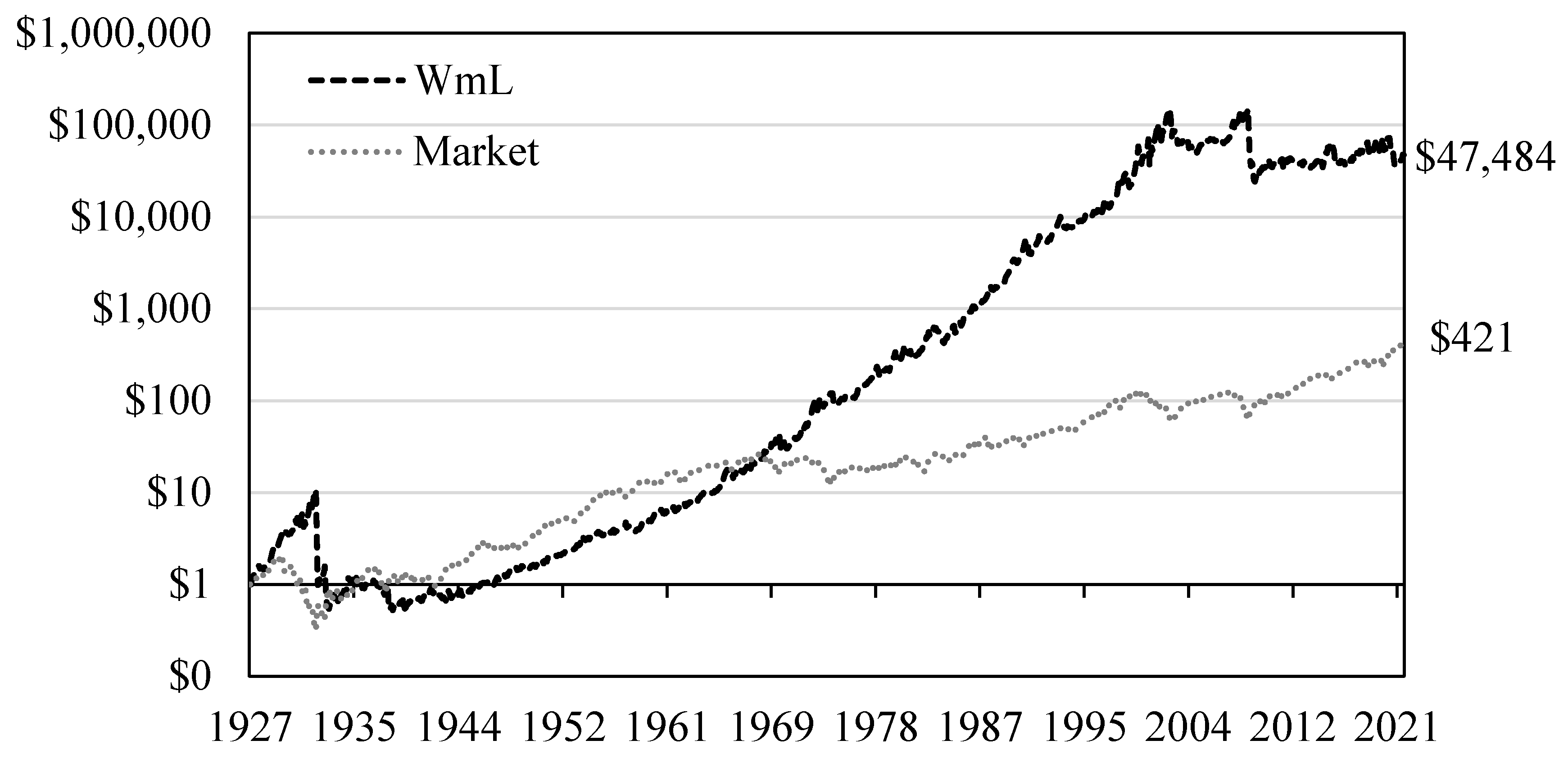
exclude transaction costs and are in line with the findings of Daniel and Moskowitz (2016). This table expands their results by adding turnover ratios, which will be fundamental to limiting the negative effects of the transaction costs. Appendix A shows how investing in the momentum portfolio significantly outperforms the stock market portfolio in the long run if transaction costs are ignored.

The high Sharpe ratio masks the effects of crashes on the momentum portfolio. Researchers who ignore the negative effects of transaction costs have praised the momentum portfolio for exhibiting a Sharpe ratio that is more than 35% greater than that of the stock market, as seen in Table 2. It is important to note that, in the Sharpe ratio, the large number of positive monthly returns decreases the importance of one very large monthly negative return. Nevertheless, it takes decades for the momentum portfolio cumulative return to recover from one crash, as seen in the black line in Appendix A.

The high stock retention rates of the first and tenth decile challenge the predictions of the Efficient Market Hypothesis and explain the existence of momentum returns. If the market prices in all the information available over the past year and all available stocks returns were classified into ten deciles, it would be reasonable to expect that the retention rate of each decile would be 10% because future price returns would depend on the arrival of independently distributed shocks. However, as seen in Table 2, only deciles three to eight have retention rates of around 10%. The retention rates of decile one (loser portfolio) and decile ten (winner portfolio) are around 55%. These high retention rates explain momentum because past overperformers tend to remain in the tenth decile and past underperformers tend to remain in the first decile.

4.2. Data: Momentum Returns with Transaction Costs (1992 to 2021)

Transaction costs should be considered, especially by covering strategies that increase the number of transactions because they are significant. Transaction costs are measured at the individual stock level as described in Equation (1). This allows us to report the price spread that each stock2 would face if it were bought and sold every month.

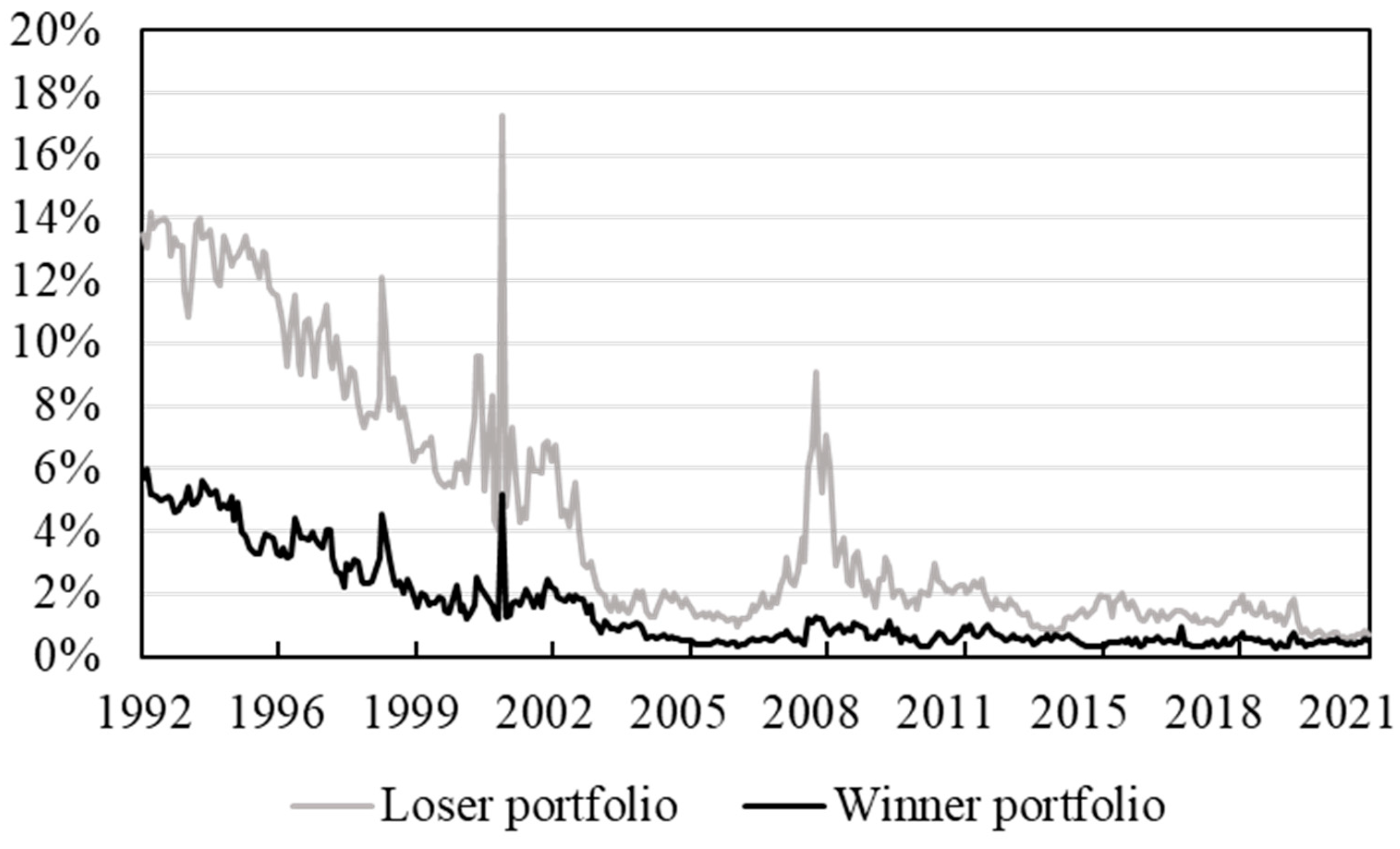
The average price spread changes significantly over time. Figure 1 displays the average round-trip cost for all the stocks in the loser and winner portfolios. The loser portfolio has consistently higher average price spreads than the winner portfolio. Overall, price spreads have decreased significantly since the early-1990s for both portfolios. Nevertheless, both portfolios faced considerable spikes in transaction costs during periods of financial stress.

Nevertheless, the negative effects of transaction cost should not be overestimated. The loser and winner portfolios are updated every month, but that does not mean that all stocks enter and leave the portfolios each month. If a stock is bought and held, or held and sold, from one month to another, the transaction cost is equal to half the price spread reported in Equation (1). Transaction costs are not paid if the stock remains in the same portfolio.

The momentum portfolio has higher expected excess returns but a lower Sharpe ratio than the market after adjusting transaction costs for turnover. As seen in

Table 3. Effect of transaction costs on momentum returns. This table shows the properties of the excess returns of the momentum, loser, winner, and market portfolios between December 1992 and December 2021. It shows the returns without transaction costs, the returns if all stocks are sold and full transaction costs are paid at the end of each month, and the returns if transaction costs are adjusted by turnover. The mean excess return, standard deviation, and Sharpe ratio (SR) are displayed in annualized percentage. The skewness (SK) and excess kurtosis (KT) are estimated from the monthly log return, ln(1+r). The variable “Crashes” shows the percentage of returns that are monthly losses larger than 5% or annualized losses larger than −46% in one month.

Return Statistic	No Transaction Costs				Transaction Costs with 100% Turnover			Returns Adjusted by Turnover
	Market	Loser (Long)	Winner (Long)	WmL	Loser (Short)	Winner (Long)	WmL	Loser (Short)	Winner (Long)	WmL
$\overline{r-r_f}$	9.19	−1.83	17.54	17.99	−16.25	11.46	−4.38	−6.32	15.79	10.99
$\sigma$	15.09	39.80	23.78	35.91	39.59	23.91	35.67	39.68	23.80	35.73
S. R.	0.61	−0.05	0.74	0.50	−0.41	0.48	−0.12	−0.16	0.66	0.31
SK	−0.95	−1.57	−0.47	−1.99	−1.52	−0.51	−2.00	−1.56	−0.48	−2.01
KT	2.43	5.92	2.60	8.39	5.63	2.68	8.50	5.87	2.60	8.58
Crashes	9.7	27.8	15.5	16.9	32.1	16.9	23.2	28.9	16.0	18.1
Turnover
Stays	100	59.40	55.50		0	0		59.40	55.50
Enters or exits	0	31.30	33.20		0	0		31.30	33.20
Enters and exits	0	9.30	11.30		100	100		9.30	11.30

The variable “Stays” shows the percentage of shares that were in the same portfolio this month as last month and will not leave the portfolio next month. “Enters or exits” shows the percentage of shares that enter the portfolio this month and will remain in the same portfolio next month or that were in the same portfolio this month as they were last month but will be in a different portfolio next month. “Enters and exists” shows the percentage of shares that were in a different portfolio last month, enter the portfolio this month, and will be in a different portfolio next month.

, between 1992 and 2021, the stock market presented an expected excess return of 9.19% and a Sharpe ratio of 0.61, and 9.7% of its returns were crashes. During the same period, the momentum portfolio without transaction costs presented an expected excess return of 17.99% and a Sharpe ratio of 0.50, and 16.9% of its returns were crashes. After adjusting by transaction costs and turnover, the momentum portfolio presented an expected excess return of 10.99% and a Sharpe ratio of 0.31, and 18.1% of its returns were crashes.

5. Stylized Facts about Momentum Returns

Covering strategies available in the literature use momentum portfolio volatility as the proxy variable to avoid momentum crashes after considering two stylized facts: First, crashes in the momentum portfolio occur at the end of a sell-off period in the stock market. Second, these periods are related to episodes of high volatility in the momentum portfolio. Appendix B shows the patterns of the fifteen largest crashes of the momentum portfolio: extreme losses arise from shorting the loser portfolio in episodes of high volatility in the loser portfolio.

However, these stylized facts are only a subset of more general properties. First, high volatility in the momentum portfolio is associated with crashes in the momentum portfolio but also with extremely high profits. Episodes of mild volatility in the momentum portfolio are associated with mild positive and mild negative returns in the momentum portfolio. Second, the ability of momentum portfolio volatility to predict extreme momentum returns comes from the information stored in the loser portfolio. Furthermore, the ability of momentum portfolio volatility to predict extreme momentum returns is undermined by the information stored in the winner portfolio.

These stylized facts can be summarized thusly: The U-shaped relationship between loser portfolio volatility and momentum returns is stronger than the U-shaped relationship between momentum portfolio volatility and momentum returns. Therefore, loser portfolio volatility is the best proxy variable to avoid momentum crashes.

5.1. Stylized Facts about Momentum Returns: U-Shaped Relationships between Momentum Returns and Volatility

The covering strategies literature has been built on the understanding that extreme negative returns are associated with episodes of high volatility. However, these stylized facts can be summarized by the U-shaped relationship between momentum returns and volatility described in this section.

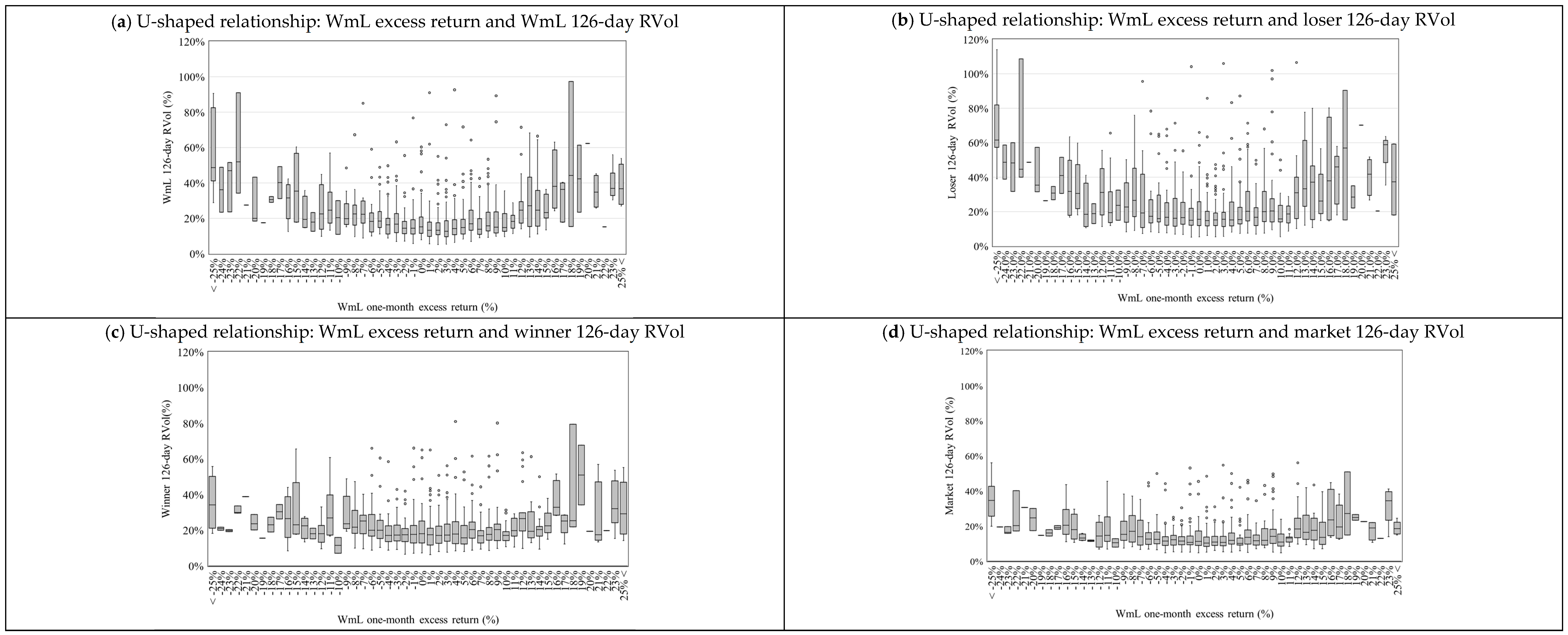
Researchers should understand the relationship between momentum returns and volatility, beyond momentum crashes, to comprehend the strengths and weaknesses of their covering strategies. There are 1134 monthly observations of momentum portfolio excess returns and the 126-day RVol of momentum, winner, loser, and market portfolios between 1927 and 2021. The results are presented after reorganizing the traditional scatter plot using a box-and-whiskers plot, as seen in Figure 2. The box-and-whiskers plot rounds momentum returns to the nearest integer. Thus, the box-and-whiskers plot displays all the variation in volatility that takes place for each 1% change in the excess returns of the momentum portfolio.

There is a U-shaped relationship between momentum returns and the volatility of different portfolios. Figure 2 shows that mild returns and mild losses in the momentum portfolio take place at the same time as low-volatility episodes in the momentum, loser, winner, and market portfolios. Also, crashes and extreme profits in the momentum portfolio tend to take place at the same time as high-volatility episodes in the momentum, loser, winner, and market portfolios.

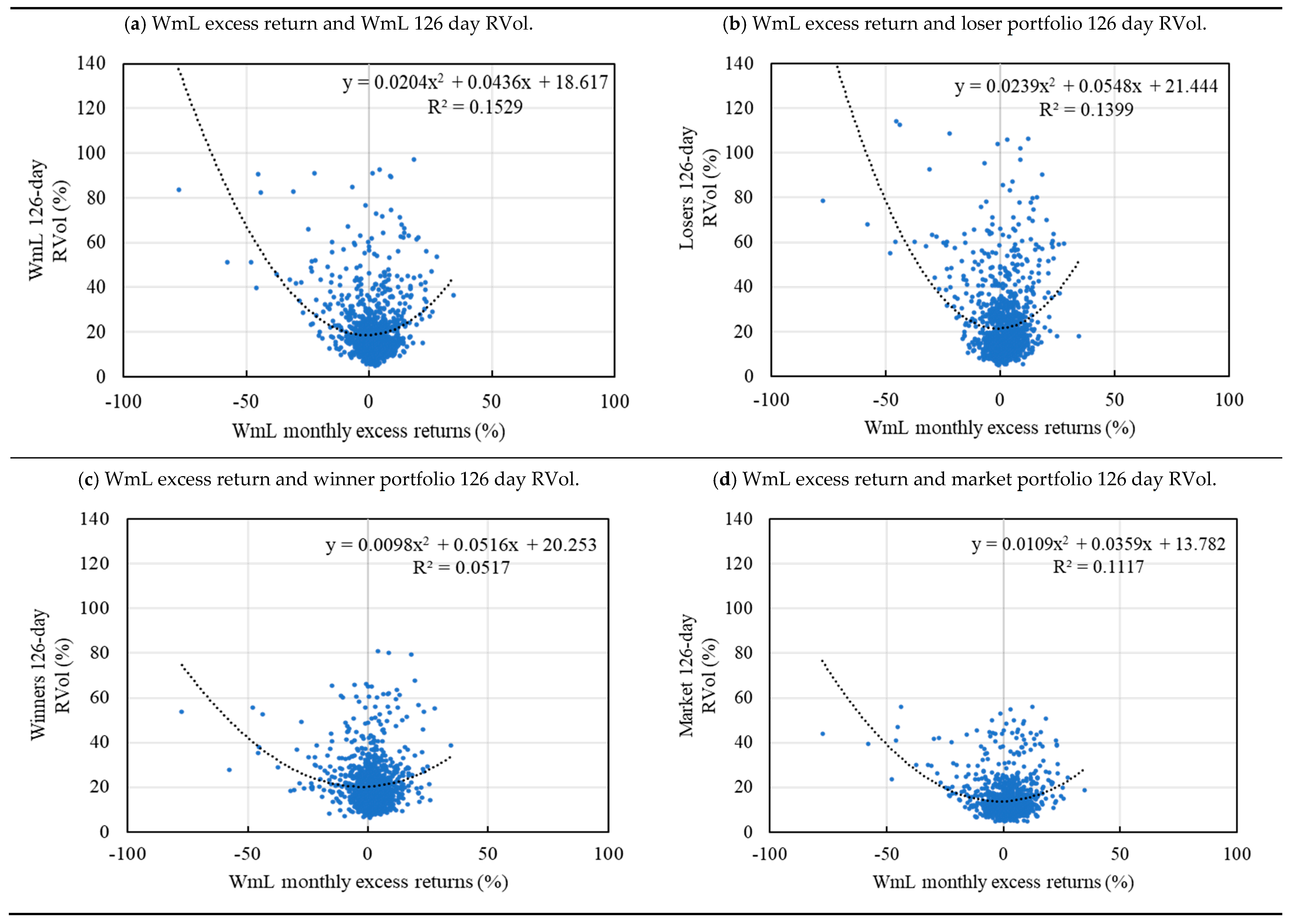
A quadratic regression is used to assess the strength of the U-shaped relationship between momentum returns and the volatility of different portfolios.

Table 4. Quadratic regression between several volatilities and momentum returns. The quadratic regression tests the U-shaped relationship between momentum returns and the realized volatility of different portfolios. The OLS regression $y={\beta }_0+{\beta }_{1}x+{\beta }_2{x}^2$ estimates the quadratic relationship between momentum excess returns, y, and the 126-day realized volatility, x, of the momentum portfolio, the loser portfolio, the winner portfolio, and the stock market. There are 1134 monthly observations between 1927 and 2021.

Model 1: $RVo{l}_{WmL}={\beta }_0+{\beta }_1{r}_{WmL}+{\beta }_2{r}_{WmL}^2$
Regression Statistics		Parameter Statistics
$R^2$	0.153	${\beta }_0$ (t-statistic)	18.62 (46.44)
Standard Error	12.46	${\beta }_1$ (t-statistic)	0.043 (0.91)
F Statistic	102.13	${\beta }_2$ (t-statistic)	0.020 (13.30)
Model 2: $RVo{l}_{Loser}={\beta }_0+{\beta }_1{r}_{WmL}+{\beta }_2{r}_{WmL}^2$
Regression Statistics		Parameter Statistics
$R^2$	0.140	${\beta }_0$ (t-statistic)	21.44 (43.41)
Standard Error	92.09	${\beta }_1$ (t-statistic)	0.054 (0.93)
F Statistic	15.35	${\beta }_2$ (t-statistic)	0.023 (12.65)
Model 3: $RVo{l}_{Winner}={\beta }_0+{\beta }_1{r}_{WmL}+{\beta }_2{r}_{WmL}^2$
Regression Statistics		Parameter Statistics
$R^2$	0.052	${\beta }_0$ (t-statistic)	20.25 (60.03)
Standard Error	30.87	${\beta }_1$ (t-statistic)	0.051 (1.28)
F Statistic	10.49	${\beta }_2$ (t-statistic)	0.009 (7.56)
Model 4: $RVo{l}_{Market}={\beta }_0+{\beta }_1{r}_{WmL}+{\beta }_2{r}_{WmL}^2$
Regression Statistics		Parameter Statistics
$R^2$	0.112	${\beta }_0$ (t-statistic)	13.78 (54.39)
Standard Error	71.16	${\beta }_1$ (t-statistic)	0.035 (1.19)
F Statistic	7.88	${\beta }_2$ (t-statistic)	0.010 (11.25)

shows that the 126-day RVols of the momentum, loser, winner, and market portfolios are used as the dependent variable in four different quadratic regressions. Each of these regressions has three parameters: ${\beta }_0$ is the intercept with the independent axis, ${\beta }_1$ represents the linear effect of the momentum excess return on the volatility, and ${\beta }_2$ represents the quadratic effect of momentum excess return on volatility.

The coefficient ${\beta }_2$ determines the direction and steepness of the curvature of the parabola. ${\beta }_2$ is statistically significant in all four regressions, which means that the excess return of the momentum portfolio has a statistically significant relationship with the volatility of the momentum, loser, winner, and market portfolios. The ${\beta }_2$ parameter is positive on all four regressions, which means that the apexes of the parabolas are at the bottom, and they open upwards.

The quadratic regressions show that the strongest U-shaped relationship is between the momentum portfolio returns and loser portfolio volatility. Figure 3 shows the parabola estimated by the quadratic equation. For example, a −77% excess return in the momentum portfolio is expected to be associated with a six-month realized volatility of 153.6% in the loser portfolio, 133.8% in the momentum portfolio, 70.3% in the market portfolio, and 69.6% in the winner portfolio. Thus, momentum returns have a stronger effect on the volatility of the loser portfolio.

The information stored in the winner portfolio volatility weakens the ability of the momentum portfolio volatility to prevent crashes. As seen in Figure 2 (bottom left), and corroborated by the third regression of Table 4, the U-shaped relationship between momentum returns and winner portfolio volatility is weak. Furthermore, the winner portfolio tends to reach episodes of higher volatility when the momentum portfolio has high returns than when it has crashes. Thus, the ability of the momentum portfolio volatility to forecast crashes in the momentum portfolio comes from the information stored in the loser portfolio volatility.

5.2. Covering Strategies: CVol Covering Strategy

The CVol covering strategy of Barroso and Santa-Clara (2015) uses the momentum portfolio 126-day RVol as a proxy because it is persistent, and it is related to momentum crashes. The weight of the CVol covering strategy is designed to buy less than one momentum portfolio the next month if the volatility of the momentum portfolio is above the target the previous month. Also, the weight buys less than one momentum portfolio the next month if the volatility of the momentum portfolio is below the previous month target, as seen in Equation (6).

Equation (6). Constant Volatility (CVol) covering strategy.

$$\begin{gathered} r_t^{CVol}=r_t^{WmL}\ast W_t^{CVol}(targe{t}_n,prox{y}_{t-1}) \\ {W}_t^{CVol}(targe{t}_n,prox{y}_{t-1})=\frac{targe{t}_n}{prox{y}_{t-1}} \end{gathered}$$

(6)

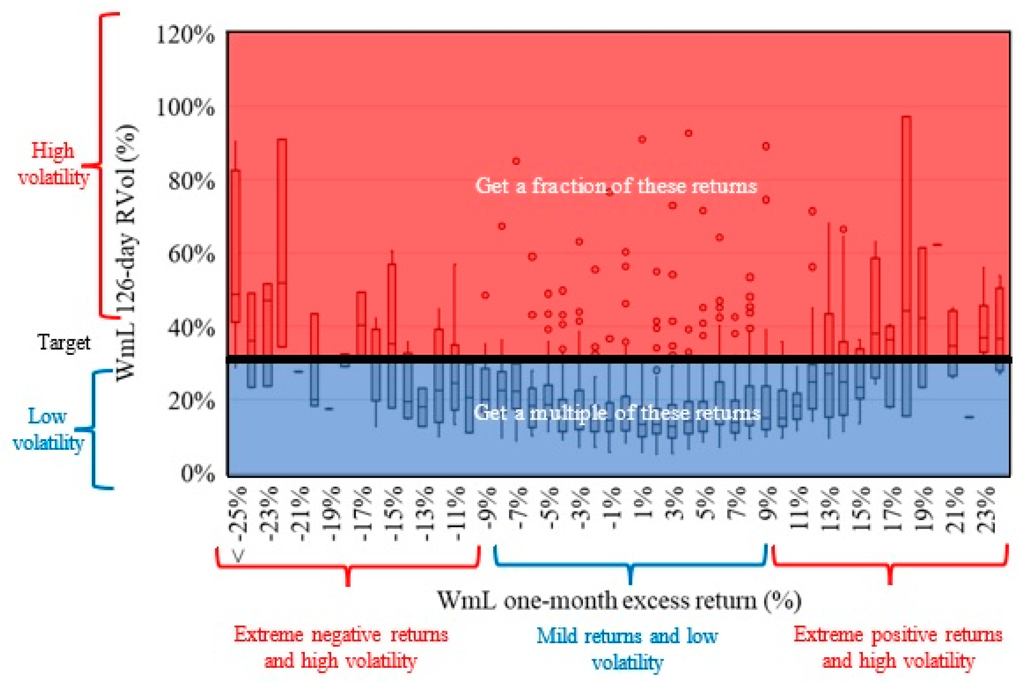
The CVol successfully mitigates the negative effects of crashes. Figure 4 shows how the CVol covering strategy interacts with the U-shaped relationship between momentum returns and momentum volatility. The solid black line shows the cutoff value (target), which differentiates between high and low volatility. The weight will be less than one for the returns that are in the red area and greater than one for returns that are in the blue area. The CVol covering strategy reduces extreme negative returns (top left corner) because it multiplies the momentum returns by a weight smaller than one.

However, the CVol also mistakenly decreases the size of large positive returns and increases the size of mild losses. The top right corner Figure 4 shows large positive returns that are associated with episodes of high volatility. In this case, the weight of the CVol is less than one, which decreases returns. The bottom center left of the same figure shows small negative returns associated with episodes of low volatility. Here, the weight of the CVol is more than one, which increases the size of mild negative returns.

However, the CVol has a compensation mechanism that masks its drawbacks. The small positive returns (Figure 4, center right) will increase because they are associated with episodes of low volatility and will be multiplied by a weight greater than one. This compensation mechanism increases the already-high positive mean of the momentum returns distribution but does not significantly reduce the heavy left tail. The CVol does not eradicate crashes; it only reduces them. Unfortunately, a fraction of the crash is still a significant loss for the portfolio.

The compensation mechanism of the CVol is successful because it ignores transaction costs. The U-shaped relationship between momentum returns and momentum volatility from Figure 4 would shift to the left if transaction costs were considered. All profits would decrease, and all losses would increase. Therefore, the negative consequences of increasing leverage when the momentum portfolio presents losses would significantly impact the performance of the CVol.

5.3. Covering Strategies: CLvg Covering Strategy

The main strength of the CLvg is that it depends only on past information. The CLvg buys the momentum portfolio when the proxy variable is below the target and buys one month of U.S. treasury bills when the proxy variable is above the target (Equation (7)). The CLvg uses the previous month’s value of the 126-day RVol of the loser portfolio as a proxy because of its strong relationship with momentum crashes, as discussed in Section 5. The target is selected using only past information.

Equation (7). Constant Leverage (CLvg) covering strategy.

$$\begin{gathered} r_t^{CLvg}=W_t^{CLvg}\ast r_t^{WmL}+\left(1-W_t^{CLvg}\right)\ast r_t^{Risk Free} \\ {W}_t^{CLvg}(targe{t}_{t-1},prox{y}_{t-1})=\left\{\begin{array}{c}1 if prox{y}_{t-1}\le targe{t}_{t-1}\\ 0 if prox{y}_{t-1}>targe{t}_{t-1}\end{array}\right. \end{gathered}$$

(7)

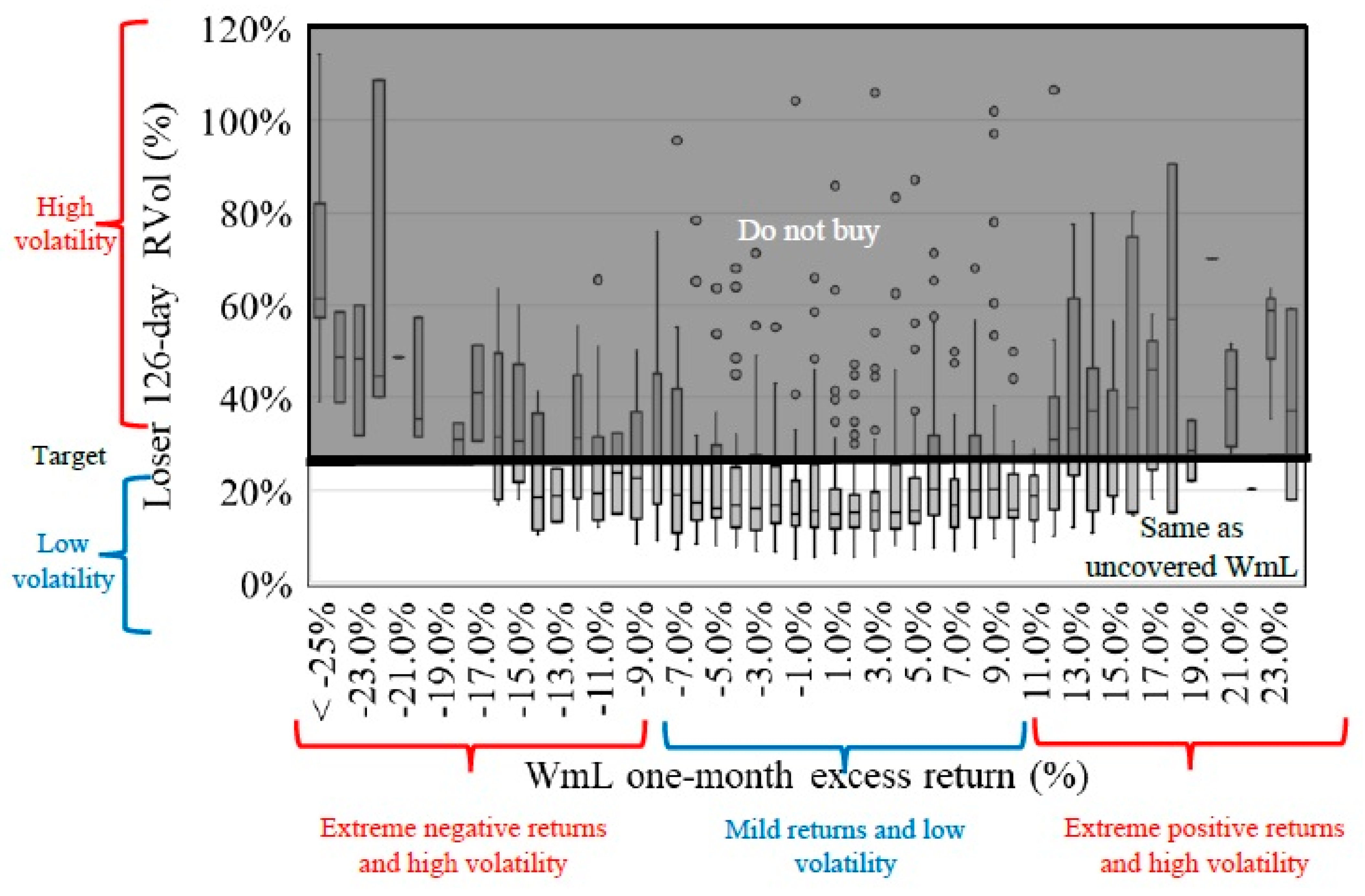
The CLvg can only increase the expected return and Sharpe ratio by forecasting and cutting more losses than profits. As seen in Figure 5, the CLvg aims to cut the tails of the momentum returns distribution (associated with episodes of high volatility) while preserving the center of the momentum returns distribution (associated with episodes of low volatility). However, the CLvg performance will improve only if it cuts the left tail more accurately than it cuts the right tail.

A strong feature of the CLvg is that it is equal to the momentum portfolio if the proxy is never greater than the target. Keeping leverage constant prevents the covering strategy from developing compensation mechanisms to cover up its shortcomings. All covering strategies will make mistakes if they do not have a forward-looking bias. The CLvg mistakenly eliminates extreme profits that are associated with episodes of high volatility. However, CLvg does not deform the center of the momentum returns distribution and does not ignore transaction costs to conceal its weaknesses.

5.4. Covering Strategies: Targets without Forward-Looking Bias

This project develops an algorithm that makes it possible to estimate a target without a forward-looking bias. It constructs an optimization grid in which each point represents a different target. The values on the grid run from zero to the highest value of the proxy. Then, for each target, the Sharpe ratio for the covering strategy over the past ten years is estimated. The target that yields the highest Sharpe ratio is selected and used as the target for the next month. The algorithm requires a rolling optimization window, so the ten-year optimization window and the optimal target for the next month are updated every month.

Under this optimization algorithm, the CLvg selects a target that is an interior solution. The CLvg is constantly facing a trade-off between increasing or decreasing the volatility threshold for the proxy variable. A high target cuts the tails of the distribution more aggressively (and prevents more crashes), but it also cuts more of the center of the distribution (which is associated with frequent mild positive returns). 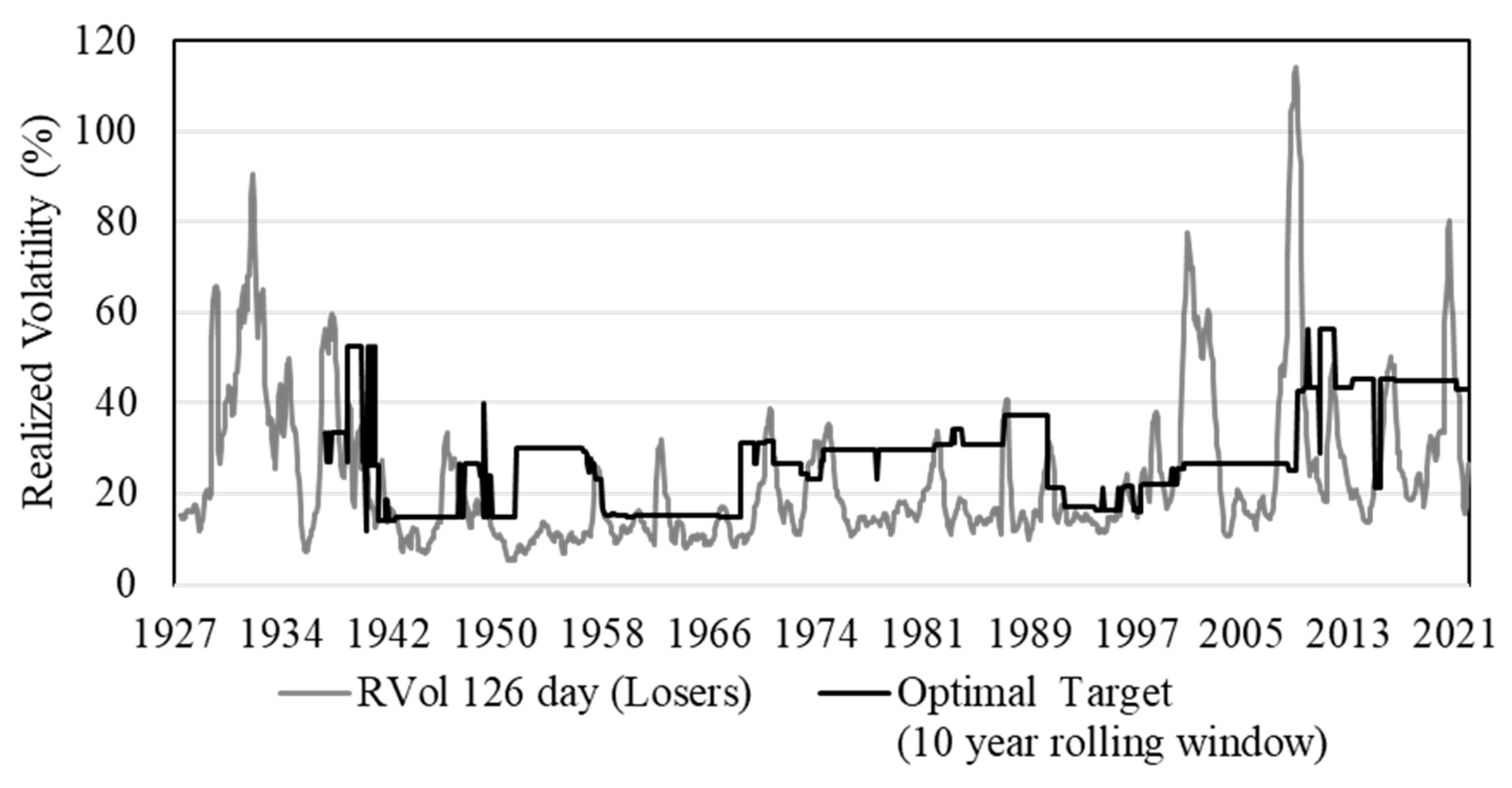Figure 6 shows the evolution of the optimal target for the CLvg while using the loser portfolio 126-day RVol as the proxy. The optimal target makes it possible to clearly distinguish between episodes of high and low volatility without the need for a forward-looking bias.

The optimal target of the CLvg shows that high loser portfolio volatility is not always bad for the momentum portfolio. From the stylized facts discussed in the previous section, only sudden and acute episodes of volatility should be targeted because they represent the culmination of periods of financial turmoil that are regularly associated with momentum crashes. As the financial turmoil ends, the aggressive market rebound will create extreme profits in the loser portfolio.

The CVol always selects a target that is a corner solution under the optimization process without a forward-looking bias. The CVol always selects the largest available target in the grid. This problem reveals the structural flaws in the design of the CVol covering strategy. The CVol can improve the Sharpe ratio without cutting more losses than profits because it does not face a restrictive trade-off. The CVol can increase the Sharpe ratio even if losses are increasing as long as profits increase at a faster rate, given its built-in compensation mechanisms. It is possible to infinitely increase the Sharpe ratio with never-ending increases in leverage, which would be impossible for practitioners to replicate.

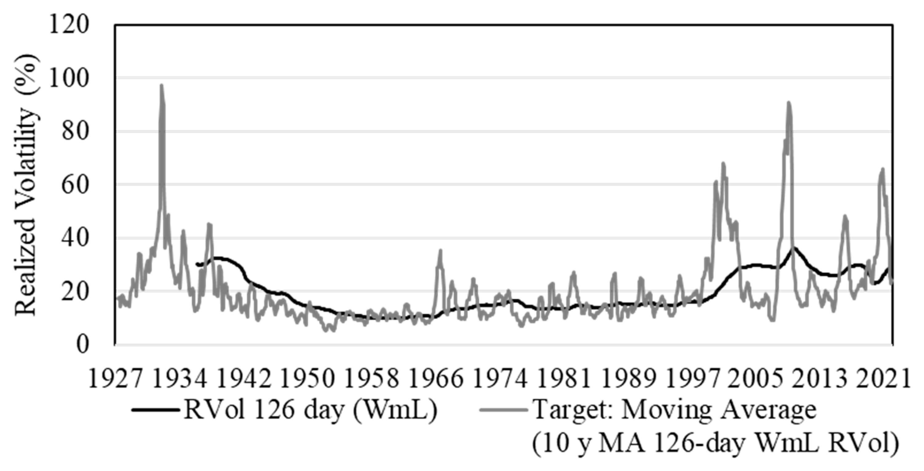
However, it is possible to select a target for the CVol without a forward-looking bias by selecting the proxy variable’s ten-year moving average as target. This is similar to setting a target equal to the sample average, as in Barroso and Santa-Clara (2015), but without a forward-looking bias. Figure 7 shows the evolution of the optimal target for the CVol with respect to the 126-day momentum portfolio RVol, which is the proxy.

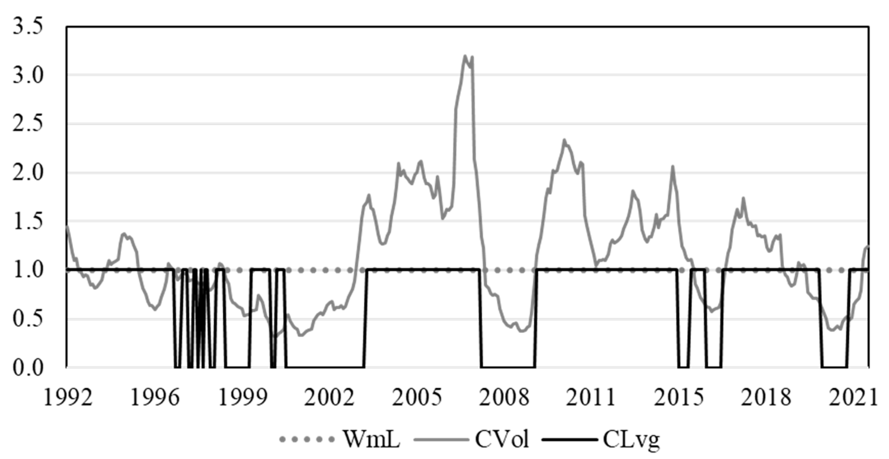
The weight summarizes a covering strategy by generating a number that adjusts the returns of the momentum portfolio after considering the interaction between the proxy and the target. Figure 8 shows the weight of CVol and CLvg. As a reference, the weight of the momentum portfolio (WmL) is always one because the leverage is not changing. The weight of the CVol is the ratio of the last month’s 126-day momentum RVol divided by the last month’s value of the ten-year moving average of the 126-day momentum RVol. The weight of the CLvg is equal to one if the last month’s 126-day loser portfolio RVol is less than the optimal target estimated from the ten-year rolling window and is zero otherwise.

5.5. Results: Implementable CVol and CLvg Strategies under Transaction Costs

The CLvg performs better than the stock market, the momentum portfolio, and the CVol even after adjusting by transaction costs at the individual stock level. The weights without forward-looking bias from Figure 8 are used to estimate portfolio returns. As seen in

Table 5. Returns statistics of several portfolios under transaction costs. This table shows the properties of the excess returns of the following portfolios for the period between December 1992 and December 2021: the stock market (Market), the momentum portfolio (WmL), the Constant Volatility (CVol) covering strategy, and the Constant Leverage (CLvg) covering strategy. The mean excess return, standard deviation, and Sharpe ratio (SR) are displayed in an annualized percentage. The skewness (SK) and excess kurtosis (KT) are estimated from the monthly log return, ln(1+r). The variable “Crashes” shows the percentage of returns that are monthly losses larger than 5% or annualized losses larger than −46% in one month. The weights are displayed in Figure 8.

Return Statistic	Market	WmL	CVol	CLvg
$\overline{r-r_f}$	9.19	10.99	16.58	16.93
$\sigma$	15.09	35.73	30.16	20.33
S. R.	0.61	0.31	0.55	0.83
SK	−0.95	−2.01	−0.71	0.26
KT	2.43	8.58	1.95	4.10
Crashes	9.74	18.05	18.62	8.31
Return USD 1	9.10	2.53	21.11	50.25

, for the period between December 1992 and December 2021, the stock market presented an average excess return of 9.19%; the momentum portfolio, 10.99%; the CVol, 16.58%; and the CLvg, 16.93%.

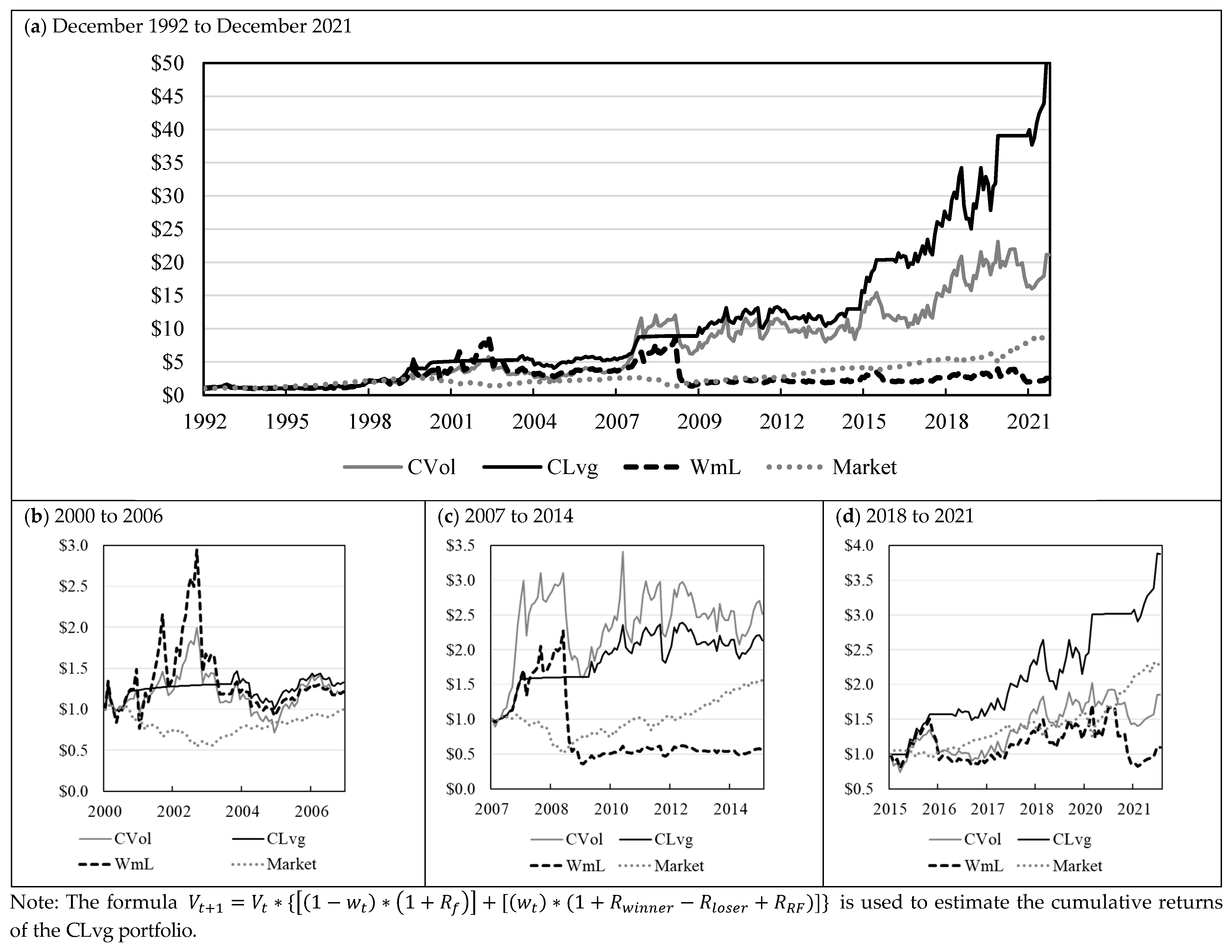
At first glance, the CVol and the CLvg have similar performances. However, the high average excess returns of the CVol disguise the outcome that almost one out of every five returns is a crash. Meanwhile, only one in twelve of the returns of the CLvg is a crash. The negative effect of a high number of crashes is better reflected in the cumulative returns for a USD 1 investment at the beginning of the period. A USD 1 investment in December 1992 would have yielded USD 21.11 on the CVol or USD 50.25 on the CLvg by December 2021.

The CVol presented losses even when it successfully predicted crashes in the momentum portfolio. Figure 9 shows the cumulative return for a USD 1 investment for several hedging strategies. The CVol successfully predicted the momentum crashes that occurred after the dot-com bubble, the Great Recession of 2008, and the COVID-19 crisis. The CVol presented fewer extreme losses than the momentum portfolio (Figure 8) because its weight was smaller than one. The problem is that buying a fraction of a crash still represents a significant loss for the CVol. Recovering from these losses required several years (Figure 9), and unrealistic increases in leverage that are not available to practitioners.

The essence of the CLvg is to avoid the momentum portfolio during the high-volatility periods that are associated with momentum crashes. The momentum portfolio is so profitable that it does not need unrealistic compensation mechanisms, like increasing leverage, if crashes are avoided. The CLvg eliminated its exposure to the momentum portfolio during the highly volatile periods following the dot-com bubble, the start of the Great Recession of 2008, and the start of the COVID-19 crisis. Instead, the CLvg bought one month of treasury bills during these volatile periods (as represented by the flat line in Figure 9). The CLvg hedging strategy does not improve the performance of the momentum portfolio by predicting the future but by avoiding highly empirically regular and forecastable episodes of high volatility in the loser portfolio that are related to momentum portfolio crashes.

5.6. Results: The Effects of Covering Strategies on the Momentum Portfolio Returns Distributions

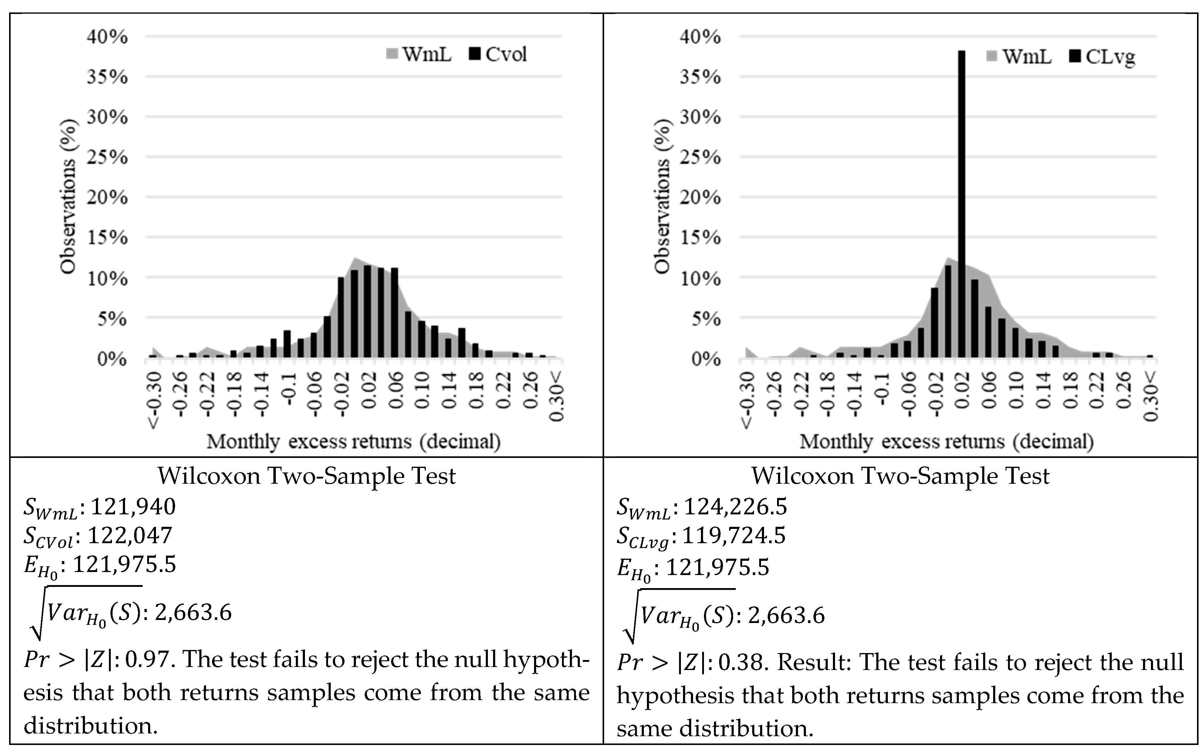
The CLvg strategy and the CVol strategy improve the performance of the momentum portfolio without significantly distorting the returns distribution. The Wilcoxon Rank-Sum Test analyzes if two distributions are statistically different. This is a non-parametric test. It does not assume that the samples have any specific distribution. It does not test if they have the same mean, or the same standard deviation, but if both come from the same distribution, as described in Appendix C. The results of Figure 10 show that the returns distributions of the CLvg strategy and the CVol strategy are statistically equal to the returns distribution of the uncovered momentum portfolio. Figure 10 shows the same results as Table 5 but in monthly returns instead of annualized returns.

The CLvg and the CVol covering strategies have minimal effects on the returns distribution of the momentum portfolio because they are able to successfully target the heavy tails of the distribution. There are not a lot of extreme-volatility episodes, but they are strongly correlated with crashes or extreme positive returns as shown in the U-shaped relationship of Section 5.1. Therefore, the covering strategies are not triggered often enough to change the whole distribution. Just avoiding some of the worst crashes has significant positive effects on the returns of the covering strategies.

Nevertheless, there are significant differences between the CVol and CLvg strategy. The CLvg eradicates the left heavy tail and moves the mass of the probability distribution from both tails to the center of the distribution, as shown in Figure 10. There is an increase in the center of the distribution from the returns that are equal to treasury bills when the CLvg hedging strategy is activated. However, they are not enough to statistically change the average and standard deviation of the distribution, because the CLvg avoids positive and negative returns that are related to extreme but infrequent volatility. Meanwhile, the CVol reduces but does not eliminate the heavy left tail of the returns distribution. This occurs because the CVol strategy buys a fraction of the crash when it predicts high volatility.

6. Conclusions

The most important contribution of the momentum returns literature has been to display the empirical limitations of the Efficient Market Hypothesis. Information stored in past monthly returns can be used to generate portfolios that outperform the stock market while exhibiting higher Sharpe ratios. Furthermore, covering strategies have shown that it is possible to use information stored in past daily returns to further increase the expected returns and Sharpe ratios of momentum portfolios.

However, the credibility of these findings had been questioned because researchers have depended on forward-looking biases to construct covering strategies and have disregarded transaction costs. Furthermore, to compensate for their mistakes, these strategies depend on deforming the momentum portfolio even in periods that do not present crashes. The covering strategies deform the momentum portfolio using unrealistically increasing leverage.

This research project develops a Constant Leverage covering strategy that depends only on past information and that accounts for transaction costs at the individual stock level. One of its most important features is that, if the proxy is smaller than the target, it behaves exactly like the momentum portfolio. These improvements are built on an understanding of momentum returns that goes beyond crashes. Momentum returns present a U-shaped relationship with the volatility of the loser portfolio. Momentum returns also present a weaker U-shaped relationship with the volatility of the momentum portfolio.

The main contribution of this project is a deeper understanding of the empirical regularities that surround momentum crashes. The future is unpredictable, and no one knows when a stock market sell-off will start or end. However, these periods of financial turmoil are marked by high volatility in the loser portfolio. These periods are predictable because the loser portfolio volatility presents high-volatility persistence and volatility clusters. A ten-year rolling window is used to find the volatility threshold at which the loser portfolio volatility is likely to predict the start of a financial crisis that will end when the momentum portfolio presents crashes.

The stylized facts of the momentum crashes documented in this paper could be used to develop new asset pricing models. Researchers have studied the Efficient Market Hypothesis and financial anomalies, but there has been little interest in developing models that merge the findings of both fields. The momentum anomaly states only that the first and tenth deciles do not behave like the EMH, but it does not contradict the Efficient Market Hypothesis in the other deciles. The momentum anomaly might be the bridge to bring the two models together.