Abstract
The aim of this study is to analyse and assess the yields and liquidity of sovereign green bonds in selected countries and to compare the yields between sovereign green bonds and conventional bonds. Sovereign green bonds are issued by governments to finance environmental and social projects and represent a relatively new and growing asset class. This study seeks to analyse the financial performance of sovereign green bonds by examining yields and liquidity metrics, such as bid–ask spreads. The findings of this research suggest that the yield to maturity (YTM) of sovereign green bonds is influenced by conventional bond return, while conventional sovereign bonds are affected by the financial market return. Furthermore, the results confirm that the liquidity of sovereign green bonds can be explained by bond maturity.
1. Introduction
Sustainable development is one of the most urgent issues discussed and analysed by governments, international organisations, and researchers. With growing pressure to transition to a low-carbon economy, the focus has also turned to the role of financial markets in achieving a green economy. The importance of green finance in creating a sustainable future was extensively discussed in the UN Climate Change Conferences in Glasgow in 2021 (COP26) and in Sharm el-Sheikh, Egypt (COP27) in 2022. At COP26, political leaders and businesses agreed on an agenda to encourage green investment and to consider climate change in every financial decision. In turn, at COP27, the significance of transforming the financial system to support investments of USD 4–6 trillion annually towards transitioning into a low-carbon economy was discussed (UN 2022). Green finance plays a crucial role in funding environmentally friendly projects and green bonds serve as important instruments for providing additional financing. The issuance of sovereign green bonds represents a proactive step towards aligning economic activities with environmental objectives, fostering a transition to a low-carbon and climate-resilient economy. By earmarking funds raised through these bonds for projects with clear environmental benefits, such as renewable energy infrastructure, sustainable transportation, or conservation initiatives, countries demonstrate their dedication to mitigating climate change and promoting environmental stewardship. Moreover, the issuance of sovereign green bonds reinforces the principles of business ethics within the government’s financial activities. By adopting transparent reporting and rigorous standards for project selection and impact assessment, countries uphold accountability and integrity in their green financing endeavours. This adherence to ethical practices not only enhances the credibility of the government in the eyes of investors and stakeholders but also sets a precedent for responsible financial management in alignment with environmental goals.
The issuance of sovereign green bonds is seen as a value-enhancing and risk-reducing behaviour by investors, providing a strong signal of a country’s commitment to a low-carbon economy (Dell’Atti et al. 2022). Green bonds can act as a mitigation mechanism for a country’s risk, attracting investors and potentially lowering the costs of financing green projects (Oche 2019). The first green bonds were created in 2007 by the World Bank and the European Investment Bank, followed by private sector in 2013–2014. The Polish government issued the first sovereign green bonds in 2016 (Jones et al. 2020).
Sovereign green bonds are a growing market in sustainable finance (Lupo-Pasini 2022) and the sovereign green bond market is expected to further expand, as more governments are adopting plans to finance sustainable growth. Since its launch, the green bond market has developed dynamically, (Mosionek-Schweda and Szmelter 2019), it is estimated that the global green bond market reached a total volume of USD 487.1 billion in 2022, with France producing the largest volume of green bonds of USD 85.4 billion. The total size of market for sovereign green bonds in 2022 was estimated to be USD 262.3 billion, with Germany being named as the largest sovereign green issuer (CBI 2022). Sovereign green bonds are typically used to fund projects that have a positive impact on the environment and contribute to the mitigation of climate change, while also generating financial returns for investors (World Bank 2022).
The aim of this paper is to analyse and evaluate the factors driving yields and liquidity in sovereign green bond markets and to compare the determinants affecting the yields of sovereign green bonds and conventional bonds. The sample includes 13 countries selected from around the world based on data availability. To the best of author’s knowledge, this is the first comprehensive study of the main factors influencing the yields and liquidity of sovereign green bonds.
Studying the liquidity and yield spread of sovereign green bonds is important because it helps to understand the overall market dynamics of a relatively new financial instrument. Additionally, understanding how green bonds perform relative to traditional bonds helps assess the impact of environmental, social, and governance (ESG) considerations on financial markets. Research on liquidity and yield spread contributes to the development of the sovereign green bond market. By identifying trends and challenges, policymakers and market participants can work towards improving market infrastructure and creating conditions for a more robust green bond market.
This study contributes to the literature in two ways. First, it examines the financial market return, conventional bond return, and yield spread as drivers of sovereign green bond yields. Second, it compares the yields between sovereign green bonds and conventional bonds. Addressing these issues enhances understanding of sustainable finance dynamics, informs investment decisions, and supports the development of policies promoting green investments.
2. Literature Review
Green bonds are fixed-income financial instruments issued to raise funds for environmentally friendly projects. Their purpose is to internalise any environmental externalities and encourage investments in green projects to achieve sustainable development (Ehlers and Packer 2017).
Sovereign green bonds are a relatively new financial instrument designed to raise capital for essential government infrastructure projects that align with the sustainable agenda. These bonds can also lower the cost of capital for environmentally friendly projects. However, the issuance of green bonds tends to be more expensive than conventional bonds due to additional administrative, legal, and marketing costs (Doronzo et al. 2021). Moreover, if the funds are not appropriately allocated, it may result in reputational damage (Climate Bonds Initiative 2018). Additionally, there is evidence that green bonds have a lower yield than conventional bonds upon issuance, known as “greenium” (Liaw 2020). Research on greenium specifically in the sovereign green bond market is limited, but Grzegorczyk and Wolff (2022) indicated the presence of a small and negative greenium in the EU sovereign bonds market. A negative greenium means that investors are willing to accept a lower return on sovereign green bonds compared to conventional bonds. One of the reasons for this is that green bonds provide an opportunity for investors to invest in green and sustainable projects. Furthermore, greenium tends to increase with AAA ratings and the issuer’s sector (Hinsche 2021). The sovereign green bond market is relatively small; it is estimated to constitute 0.2 percent of all government securities in Organisation for Economic Co-operation and Development (OECD) countries and sovereign green bonds issuance accounts for 12 percent of all green bond issuances in emerging economies (Sakai et al. 2022). However, the sovereign green bond market is growing, driven by the increasing demand for environmentally sustainable economics.
The literature on sovereign green bonds, although limited, is expanding and can be categorised into the following segments: the impact of green bond issuance on different stakeholders, the influence of green bond issuance on the cost of capital, greenwashing through the issuance of green bonds, the theoretical foundation of green bonds, and factors affecting the green bond market (Cortellini and Panetta 2021). This paper aims to contribute to the analysis of the determinants of green bonds’ liquidity and yields, which falls within the broader strand of the literature on green bonds.
One of the main factors that can influence the green bond market are macroeconomic indicators. For example, a study by Tolliver et al. (2019) demonstrated that these factors can exert a greater influence on the green bond market compared to institutional influences. Similarly, Broadstock and Cheng (2019) provided evidence of the significance of macroeconomics indicators for the growth of the green bond market.
The financial market can also influence the green bond market. Reboredo et al. (2020) studied the relationship between the volatility of green bonds and other financial instruments and found evidence of the co-movement of green bond price with high-yield bonds and energy stocks. On the other hand, Dell’Atti et al. (2022) analysed the relationship between the issuance of sovereign green bonds and the country stock and CDS (credit default swap) market in EU countries. Both the stock market and CDS market responded positively to the announcement of issuance of sovereign green bonds, sending a strong signal to environmentally friendly investors.
Doronzo et al. (2021) focused on conventional bonds and sovereign green bonds and concluded that there is no price difference between the two assets. However, several studies, including Ehlers and Packer (2017); Hachenberg and Schiereck (2018); Zerbib (2019); Gianfrate and Peri (2019); and Nanayakkara and Colombage (2019) have reported that green bonds trade at a lower yield (higher price) than conventional bonds.
Mosionek-Schweda and Szmelter (2019) conducted a comparative analysis of the sovereign green bonds issued in different countries and discovered significant differences in the yields of sovereign green bonds between countries. However, their study does not explain the causes of these differences.
This paper aims to fill the gap in research and examine the main factors affecting yields and liquidity among the 13 countries involved in the issuance of sovereign green bonds. It represents the first study to provide a comprehensive analysis of sovereign green bond yields and liquidity, as well as to compare the yields between sovereign green bonds and conventional bonds.
The financial markets are generally efficient (Fama 1970), meaning that security prices reflect all available information. This means that asset prices, including security prices, quickly adjust to reflect all available information and it is difficult or impossible for investors to consistently achieve returns above the average market returns. Under the efficient market hypothesis, bond yields would swiftly incorporate market developments and economic indicators. These include changes in interest rates, inflation expectations, and overall economic conditions. Essentially, any new information regarding the economic outlook or market conditions would be rapidly reflected in bond yields. This implies that sovereign green bond and conventional bond yields are both subject to the swift integration of market developments and economic indicators. As a result, the efficient market hypothesis suggests that sovereign green bond yields would respond to market developments and economic indicators in a similar manner to conventional bonds. Hence, two hypotheses have been formulated.
Hypothesis 1.
The yields of sovereign green bonds are influenced by market developments and the economic outlook. A positive economic outlook increases the YTM of green sovereign bonds.
Hypothesis 2.
Both sovereign green bonds and conventional bonds will be influenced by market development and the economic outlook in a similar manner.
Additionally, the market microstructure theory, according to which the liquidity of a specific asset, such as sovereign green bonds, is influenced by factors such as trading volume, bid–ask spreads, and market depth. Furthermore, the maturity of sovereign green bonds can also influence their liquidity. Shorter-maturity bonds may be more liquid than longer-term bonds due to lower price volatility and higher trading activity in the short end of the yield curve. Also, as the overall performance of the financial markets, as reflected in market indices such as stock market returns or bond market indices, can impact investor sentiment and risk appetite, thereby affecting the liquidity of sovereign green bonds. This is the basis for Hypothesis 3.
Hypothesis 3.
The main drivers of sovereign green bonds’ liquidity are the liquidity of benchmark bonds, yield spread, green bond maturity, and financial market return.
3. Data and Methodology
The empirical analysis in this study will include the green bonds issued by 13 governments, namely Belgium, Chile, Egypt, France, Germany, Italy, Lithuania, Netherlands, Nigeria, Poland, Serbia, Spain, and the UK. Data were collected daily from 17 September 2021 until 29 April 2022 (Appendix A, Table A1) from the Thomson Reuters database. The time period of September 2021 to April 2022 encompasses a significant duration of eight months, especially considering that the data are collected daily. This period captured various market developments, policy changes, and environmental events that may affect the performance and perception of sovereign green bonds. Selecting a relatively recent time period ensures that the research findings reflect the most up-to-date information and market conditions that can potentially affect green bond yields and liquidity. Another rationale for selecting this period was the availability of the data to ensure that the widest sample of countries is included.
The panel regression model will be estimated to analyse the drivers of profitability and liquidity of sovereign green bonds. Panel regression models offer a comprehensive framework for analysing data with both cross-sectional and time-series dimensions, providing insights into individual-specific effects, trends over time, and dynamic relationships among variables. In this model, the dependent variable is the yield to maturity of conventional bonds in selected countries.
The fixed-effects estimation method will be employed to estimate panel data models. The fixed-effects model was selected based on the Hausman test presented in Table A3 in Appendix A. The null hypothesis of the Hausman test states that random effect is a preferred model, and as the p-value is below the critical value, the fixed-effect model was selected.
In the literature, the main indicators used to measure the financial performance of green bond yields are the current yield (CY), yield to maturity (YTM), or bond prices (Mosionek-Schweda and Szmelter 2019; Russo et al. 2020). In this study, YTM will be used as the dependent variable because it is an important measure in financial analysis for evaluating investments. YTM represents the compound return rate that investors will receive if they hold the bond until maturity (Gebhardt et al. 2005; Muhammad and Masron 2009).
There are significant differences in the level of the yield to maturity (YTM) among countries in the sample. Egypt had the highest YTM in the selected period. Nigeria ranked second, followed by Egypt, Italy, Chile, UK, Spain, Poland, France, Lithuania, Belgium, and the Netherlands (Table 1). On the other hand, securities issued by Germany exhibited relatively low yield indicators (Table 1).

Table 1.
Descriptive statistics for bid yield of green bonds.
Table 1 presents the descriptive statistics for bid yield for all the countries in the sample from 17 September 2021 until 29 April 2022. Data were obtained from the Thomson Reuters database. Additionally, Table 2 presents Pearson correlation matrix to confirm that there is no problem with multicollinearity.
Table 2.
Pearson correlation matrix.
Additionally, the majority of countries in the sample exhibit relatively stable yield to maturity (YTM) for their green bonds, with the exception of Egypt, Nigeria, and Serbia, which have a relatively variable YTM for their green bonds (Figure 1).
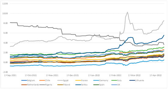
Figure 1.
Yield to maturity over time across all countries.
In order to test for the presence of a unit root in the bid yields of green bonds, the Levin et al. (2002) test (LLC) test was applied. The LLC proposes the test in which the homogeneity of the rho is assumed:
The results of the LLC test presented in Table A2 in Appendix A indicates that the green bond bid yield variable is stationary. To further contribute to the diagnostic process of regression errors, Durbin–Watson tests were conducted. The results of the Durbin–Watson tests, presented in Appendix A, Table A5, indicate that there is no autocorrelation in the residuals, as the results of the tests are around values of 2.
In addition, we conducted the Breusch–Pagan test to examine heteroscedasticity. The results from Appendix A, Table A6, indicate the presence of heteroscedasticity. Consequently, robust errors will be utilised in all regressions to address this.
Figure 1 presents the yield to maturity for all the countries in the sample in the period between 17 September 2021 until 29 April 2022. Data are obtained from the Thomson Reuters database.
To examine the potential impact of macroeconomic factors on green bond bid yields, the regression model will include the yield spread, calculated as the difference between long-term sovereign bonds and short-term sovereign bonds. The yield spread is widely recognised in the literature as an indicator of real economic activity (Kanagasabapathy and Goyal 2002; Estrella and Mishkin 1996). A flat or negative slope for the yield curve is considered a signal of a future economic recession since it reflects the effects of monetary policy. Monetary contraction can result in an increase in nominal short-term interest rates, leading to a flat or negative yield spread. Additionally, high real interest rates can adversely affect investment, potentially contributing to a future recession.
Furthermore, we aim to examine the relationships between financial market return, conventional bond market return, and green bond yields. The financial market return is based on the Refinitiv Price Return Index for each country in sample.
To further examine whether financial market variables, yield spread, and bond return may have lagged effects on the sovereign green bond’s yields, these variables will be included with a first lag. By including lagged variables in the regression, delayed responses can be captured. Lagged variables can help capture the evolving nature of these relationships over time, allowing for a more nuanced analysis of how changes in financial market conditions affect the dependent variable.
where:
y: green bond yield to maturity
: calculated as a difference between long-term sovereign bonds and short-term sovereign bond
: financial market price return
: the market return is calculated as the mid-price return of the individual sovereign bonds (conventional) in a country
: error terms
To assess whether the selected variables can similarly affect the returns of sovereign green bonds and conventional sovereign bonds, an additional panel regression model has been included.
where:
y: conventional bond yield to maturity
: calculated as a difference between long-term sovereign bonds and short-term sovereign bonds
: financial market price return
: the bond return is calculated as the mid-price return of the individual sovereign bonds (conventional) in a country
: error terms
To analyse factors affecting sovereign green bond liquidity, we will use the bid–ask spread as the dependent variable (Table 3), as it is a commonly used proxy for bond liquidity in the literature (Richter 2022; Langedijk et al. 2018; Febi et al. 2018). To investigate the key drivers of sovereign green bond liquidity, we included bond characteristics variables such as maturity, as this has an important influence on liquidity. For instance, Dick-Nielsen et al. (2012) found evidence that liquidity increases with maturity for corporate bonds. Similarly, Su and Tokmakcioglu (2021) found that short maturity narrows the bid–ask spread.
Table 3.
Green bond bid yield descriptive statistics.
Table 3 reports descriptive statistics on green bonds’ yield spread for all the countries in the sample in the period between 17 September 2021 and 29 April 2022. Data are obtained from the Thomson Reuters database.
Furthermore, we include yield spread as an indicator of the economic outlook, as well as financial market variables, namely financial market return and conventional sovereign bond return.
Lastly, we test whether the liquidity of conventional sovereign bonds can affect green bond liquidity. To further examine whether financial market variables, yield spread, and bond return may have lagged effects on the liquidity of sovereign green bonds, these variables will be included with a first lag.
y: bid–ask spread calculated as the difference between bid and ask yield
: the liquidity of the sovereign bond (conventional) market
: calculated as a difference between long-term sovereign bonds and short-term sovereign bond
: the market return is calculated as the equally weighted average of the continuous mid-price return of the individual sovereign bonds (conventional) in a country
: financial market price return
: days to maturity of sovereign green bonds
: error terms
4. Results and Discussion
The results presented in Table 4 reveal a negative correlation between conventional sovereign bond return and bond return in the first lag and the yield to maturity (YTM) of green bonds. A negative relationship between conventional sovereign bond returns and the YTM of green bonds suggests that green bonds tend to offer higher yields or become relatively more attractive compared to conventional bonds during periods of declining conventional bond returns. For example, Abakah et al. (2022) study showed a strong connectedness between green bonds and conventional sovereign bonds, particularly during economic downturns. The connection between conventional and green bonds is multifaceted and influenced by various factors such as the bond rating and issuing currency (González-Fernández and González-Velasco 2018).
Table 4.
Green bonds bid yields regression results. Fixed-effect model.
The results presented in Table 5 reveal a negative correlation between financial market returns and the yield to maturity (YTM) of green bonds. The existing literature offers differing views and evidence regarding the relationship between stock and bond returns. Some studies suggesting a positive correlation between the financial market and bond market have emphasised that both markets are exposed to the same macroeconomic factors, which in turn affect both markets in a similar manner. Empirical studies by Keim and Stambaugh (1986), Campbell and Ammer (1993), Kwan (1996), and d’Addona and Kind (2006) have provided supportive evidence in this regard.
There are also studies that suggest that a negative correlation between two assets can be observed during times of high volatility or fall in the financial market (Gulko 2002; Connolly et al. 2005; Andersson et al. 2008; Baur and Lucey 2009). This can be explained by the ‘flight to quality’ phenomenon, where investors prefer to invest in safer assets in the event of a decline in the financial market and ‘flight-from-quality’ phenomena, where investors become less risk averse and invest in the financial market rather than in bonds during a rise in financial market.
The regression analysis presented in this paper also controls for one-period lagged financial market variables. The results suggest that the lagged variables have a similar effect on the YTM of green bonds as the non-lagged variables.
Table 5.
Conventional bond bid yields regression results. Fixed-effect model.
Table 5.
Conventional bond bid yields regression results. Fixed-effect model.
| (1) | (2) | (3) | (4) | |
|---|---|---|---|---|
| Yield spread | 0.1547 (0.1196) | 0.1125 (0.0795) | ||
| Financial market | −0.0082 *** (0.0012) | −0.0085 *** (0.0013) | −0.0054 *** (0.0009) | |
| Yield spread lag | 0.1521 (0.1182) | 0.1516 (0.1180) | 0.0412 (0.0569) | |
| Financial market lag | −0.0083 *** (0.0013) | −0.0030 *** (0.0007) | ||
| Bond return | −2.0834 * | −1.9275 | −1.8841 | |
| (1.0385) | (1.2671) | (1.0649) | ||
| Bond return lag | −1.8994 | −1.2730 | ||
| (1.0111) | (0.8655) | |||
| R-squared | 0.2874 | 0.2889 | 0.2866 | 0.2935 |
| Observations | 2009 | 1996 | 1997 | 1940 |
Table 5 presents the regression results for conventional bond bid yields. The unbalanced pooled data were observed daily for a panel of 13 countries over the period between 17 September 2021 and 29 April 2022. Yield spread lag is one-day-lagged yield spread. Financial market lag is one-day-lagged financial market return, and bond return lag is one-day-lagged bond return. The asterisks ***, and * denote statistical significance at the 0.1%, and 5% levels, respectively. Standard errors are shown in parentheses beneath the regression coefficients.
The results presented in Table 6 suggest that green bond liquidity can be explained solely by green bond maturity, as the other variables are not statistically significant. The maturity coefficients are positive but small, indicating that liquidity increases with the maturity of green bonds. The results indicate that the inclusion of lagged variables in addition to non-lagged variables does not have a significant impact on green bond liquidity. However, when only lagged variables are included, the influence on green bond liquidity is very similar to the regression results with only non-lagged variables.
Overall, the shorter-term bonds generally exhibit higher liquidity compared to longer-term bonds, but the relationship between bond liquidity and maturity is nuanced and can be influenced by a variety of factors, including investor preference, market conditions, yield curve dynamics, and issuer credit risk. Furthermore, research confirms a positive relationship between maturity and green bond liquidity. For example, the study by Boutabba and Rannou (2020) indicated that that for European green bonds, liquidity premiums increase with bond maturity, with long-term investors being compensated for higher illiquidity risks.
Table 6.
Green bond liquidity regression results. Fixed-effect model.
Table 6.
Green bond liquidity regression results. Fixed-effect model.
| (1) | (2) | (3) | |
|---|---|---|---|
| Yield spread | 0.0110 (0.0097) | 0.0179 (0.0172) | |
| Financial market | −0.0009 (0.0011) | −0.0008 (0.0011) | |
| Bond return | −0.0585 (0.0982) | −0.0193 (0.0655) | |
| Liquidity | 0.7298 (0.6651) | 0.7125 (0.6406) | 0.7607 (0.6811) |
| Maturity | 0.0003 ** (0.0001) | 0.0003 ** (0.0001) | 0.0003 ** (0.0001) |
| Yield spread lag | −0.0073 (0.0089) | 0.0104 (0.0087) | |
| Financial market lag | −0.0009 (0.0012) | ||
| Bond return lag | −0.0922 (0.1122) | ||
| R-squared | 0.1034 | 0.1092 | 0.10983 |
| Observations | 2003 | 1934 | 1991 |
Table 6 presents the regression results for green bond liquidity. The data were observed daily for a panel of 13 countries over the period between 17 September 2021 and 29 April 2022. Yield spread lag is one-day-lagged yield spread. Financial market lag is one-day-lagged financial market return, and bond return lag is one-day-lagged bond return. The asterisks ** denote statistical significance at the 1%, and 5% levels, respectively. Standard errors are shown in parentheses beneath the regression coefficients.
Robustness
To ensure the robustness of the results, we conducted a series of additional tests. Specifically, we employed green bond mid-yield as the dependent variable to assess green bond yields and conventional bond bid yield as the independent variable to analyse conventional bond return. These variables were included in a fixed-effects panel regression to estimate the relationships.
The results of the robustness test, as shown in Table 7, confirm of the main regression results. In order to assess the robustness of the liquidity regression results, a different measure of green bond liquidity was employed. Green bond liquidity was calculated by dividing the bid–ask spread by the mid-price, following the methodology used by Langedijk et al. (2018).
Table 7.
Robustness checks on the green bond yield regression results.
The robustness test results presented in Table 8 confirm the findings of the original regression results, as the maturity remained statistically significant. However, the correlation coefficients from the robustness test indicated a relatively weaker effect compared to the original regression estimation. Additionally, the alternative liquidity measure is statistically significant, indicating a positive relationship between conventional bond liquidity and green bond liquidity.
Random-effect regression was also included to assess if there was an endogeneity problem. The coefficients from both the fixed-effect and random-effect regressions, presented in Table 4 and Table 9 for the green bond bid yields regression, Table 5 and Table 11 for conventional bond bid yields regression, and Table 6 and Table 13 for green bond liquidity regression, are similar in significance and magnitude. This similarity indicates that there is no problem with the correlation of the explanatory variables with the error terms.
Table 8.
Robustness checks for the green bond liquidity regression results.
Table 8.
Robustness checks for the green bond liquidity regression results.
| (1) | (2) | (3) | |
|---|---|---|---|
| Liquidity different measure | 0.3549 *** (0.0994) | 0.3474 *** (0.0974) | 0.3521 *** (0.0990) |
| Yield spread | 0.0001 (0.0001) | 0.0002 (0.0002) | |
| Bond return | 0.0007 (0.0015) | 0.0011 (0.0015) | |
| Financial market | 0.0000 (0.0000) | 0.0000 (0.0000) | |
| Yield spread lag | −0.0001 (0.0001) | 0.0001 (0.0001) | |
| Financial lag | 0.0000 (0.0000) | 0.0000 (0.0000) | |
| Maturity | 0.0000 * (0.0000) | 0.0000 * (0.0000) | 0.0000 * (0.0000) |
| Bond return lag | 0.0007 (0.0024) | −0.0003 (0.0020) | |
| R squared | 0.2248 | 0.2288 | 0.2334 |
| Observations | 2009 | 1940 | 1997 |
Table 8 presents a robustness check on the regression results for green bond liquidity. The data were observed daily for a panel of 13 countries over the period between 17 September 2021 and 29 April 2022. Yield spread lag is one-day-lagged yield spread, and financial market lag is one-day-lagged financial market return. The asterisks ***, and * denote statistical significance at the 0.1% and 5%, levels, respectively. Standard errors are shown in parentheses beneath the regression coefficients.
Additionally, to check the robustness of the results to the regression model, random-effect and pooled regression models were used; the results are presented in Table 9, Table 10, Table 11, Table 12, Table 13 and Table 14. The random-effect model confirmed the fixed-effect results, while the pooled-effect model did not confirm the fixed-effect results. One potential explanation for the inconsistency between the fixed- and pooled-effect results is that the pooled regression treats all observations equally and does not account for potential heterogeneity across individuals or groups.
Table 10.
Green bond bid yield regression results. Pooled regression.
Table 11.
Conventional bond bid yield regression results. Random-effect model.
Table 12.
Conventional bond bid yield regression results. Pooled regression.
Table 13.
Green bond liquidity regression results. Random-effect model.
Table 14.
Green bond liquidity regression results. Pooled regression.
Table 9.
Green bond bid yield regression results. Random-effect model.
Table 9.
Green bond bid yield regression results. Random-effect model.
| (1) | (2) | (3) | (4) | |
|---|---|---|---|---|
| Yield spread | −0.0232 (0.1740) | 0.0344 (0.2036) | ||
| Financial market | −0.0097 (0.0007) | −0.0033 (0.0027) | −0.0097 (0.0051) | |
| Bond return | −3.8151 * (1.6864) | −4.0383 (2.5563) | −3.6075 (1.9752) | |
| Yield spread lag | −0.0297 (0.1709) | −0.036 (0.2154) | −0.0259 (0.1729) | |
| Financial market lag | −0.0096 (0.0051) | −0.0014 (0.0009) | ||
| Bond return lag | −3.6339 ** (1.4064) | −3.3345 (2.0609) | ||
| R-squared | 0.0848 | 0.0826 | 0.05387 | 0.08435 |
| Observations | 2009 | 1997 | 1940 | 1996 |
Table 9 presents the regression results for green bond bid yields. The unbalanced pooled data were observed daily for a panel of 13 countries over the period between 17 September 2021 and 29 April 2022. For Nigeria, mid-yield was used. Yield spread lag is one-day-lagged yield spread. Financial market lag is one-day-lagged financial market return, and bond return lag is one-day-lagged bond return. The asterisks **, and * denote statistical significance at the 1%, and 5% levels, respectively. Standard errors are shown in parentheses beneath the regression coefficients.
5. Conclusions
This study is one of the first to comprehensively analyse the return and liquidity of sovereign green bonds. The analysis in this paper presents evidence that the YTM of green bonds is influenced by conventional bond return, whereas sovereign conventional bonds are affected by financial market return.
Additionally, the presented results show that the liquidity of green bonds can be explained by green bond maturity. Furthermore, the robustness tests conducted for both the green bond yields and liquidity confirmed the main findings. This strengthens the validity and reliability of the results and provides more confidence in the implications drawn from the study.
Overall, the study’s findings contribute to a deeper understanding of the return and liquidity aspects of sovereign green bonds. This has implications for investors, policymakers, and financial markets participants.
For investors, the study provides important insights into the behaviour of sovereign green bonds compared to that of conventional bonds. A negative relationship indicates that green bonds tend to offer higher yields compared to conventional sovereign bonds when conventional bond returns decrease. Investors may perceive green bonds as offering better returns or risk-adjusted returns during periods of market downturns or declining interest rates.
Participants in the financial markets, including bond issuers and underwriters, can use the study’s insights to make informed decisions. Understanding the factors that influence green bond yields and liquidity can guide bond structuring and issuance strategies.
While this study provides valuable insights into the return, risk, and liquidity aspects of sovereign green bonds, there is a scope for future research. A larger and more diverse sample could provide a more comprehensive understanding of the sovereign green bond market. Additionally, extending the time frame can capture longer-term trends or structural changes in the sovereign green bond market. Moreover, metrics related to the environmental impacts of the projects funded by green bonds could be also considered.
Funding
This research received no external funding.
Informed Consent Statement
Not applicable.
Data Availability Statement
The raw data supporting the conclusions of this article will be made available by the authors on request.
Conflicts of Interest
The author declares no conflict of interest.
Appendix A
Table A1.
Data sources.
Table A1.
Data sources.
| Variable | Definition | Source |
|---|---|---|
| Green bond bid and ask yield | Calculated as the difference between bid and ask yield | Thomson Reuters database |
| Yield spread | Calculated as a difference between long-term sovereign bonds and short-term sovereign bonds | Thomson Reuters database |
| Financial market return | Financial market price return | Financial market price return index Thomson Reuters database |
| Green bond YTM | Green bond yield to maturity | Thomson Reuters database |
| Conventional bond return | Calculated as the equally weighted average of the continuous mid-price return of the individual sovereign bonds (conventional) in a country | Thomson Reuters database |
| Conventional bond YTM | Conventional bond yield to maturity | Thomson Reuters database |
| Maturity | Days to maturity of sovereign green bonds | Thomson Reuters database |
| Liquidity | Calculated as the difference between bid and ask yield of conventional bonds | Thomson Reuters database |
Table A2.
LLC test results for green bond bid yield.
Table A2.
LLC test results for green bond bid yield.
| z value | −6.502 |
| p value | 3.963 × 10⁻¹¹ |
Table A3.
Hausman test.
Table A3.
Hausman test.
| Regression | Green Bonds Bid Yields Regression | Conventional Bond Bid Yields Regression | Green Bond Liquidity Regression |
|---|---|---|---|
| Chi-squared | 129.19 | 181.36 | 518.2 |
| p-value | 2.2 × 10⁻¹⁶ | 2.2 × 10⁻¹⁶ | 2.2 × 10⁻¹⁶ |
| Degree of freedom | 6 | 4 | 4 |
Table A4.
Sovereign green bond issuance.
Table A4.
Sovereign green bond issuance.
| Country | Green Bond Issuance Date | Green Bond Maturity Date |
|---|---|---|
| Belgium | 27 February 2018 | 22 April 2033 |
| Chile | 26 January 2019 | 2 July 2031 |
| Egypt | 30 September 2020 | 6 October 2025 |
| France | 1 January 2018 | 25 June 2039 |
| Germany | 4 November 2020 | 10 October 2025 |
| Italy | 4 March 2021 | 30 April 2045 |
| Lithuania | 18 May 2018 | 3 May 2028 |
| Netherlands | 22 May 2019 | 15 January 2040 |
| Nigeria | 11 April 2018 | 22 December 2022 |
| Poland | 1 February 2018 | 7 August 2026 |
| Serbia | 17 September 2021 | 23 September 2028 |
| Spain | 8 September 2021 | 30 July 2042 |
| UK | 15 September 2021 | 31 July 2033 |
Table A5.
Durbin–Watson test for autocorrelation.
Table A5.
Durbin–Watson test for autocorrelation.
| Green Bond Bid Yields Regression | Conventional Bond Bid Yields Regression | Green Bond Liquidity Regression | |
|---|---|---|---|
| specification 1 | 2.517 | 2.5579 | 2.1093 |
| specification 2 | 2.5149 | 2.5562 | 2.1222 |
| specification 3 | 2.4948 | 2.5607 | 2.1221 |
| specification 4 | 2.5154 | 2.5675 | 2.1067 |
Table A5 presents the Durbin–Watson test results.
Table A6.
Breusch–Pagan test for heteroscedasticity.
Table A6.
Breusch–Pagan test for heteroscedasticity.
| Green Bond Bid Yield Regression | Conventional Bond Bid Yields Regression | Green Bond Liquidity Regression | |
|---|---|---|---|
| specification 1 | 41.796 *** | 52.961 *** | 228.89 *** |
| specification 2 | 42.451 *** | 52.676 *** | 248.65 *** |
| specification 3 | 40.197 *** | 52.713 *** | 249.01 *** |
| specification 4 | 42.26 *** | 52.092 *** | 256.24 *** |
Table A6 presents the results of the Breusch–Pagan test for heteroscedasticity. The asterisks ***, denote statistical significance at the 0.1%, levels, respectively.
References
- Abakah, Emmanuel Joel, Aviral Kumar Tiwari, Aarzo Sharma, and Dorika Jeremiah Mwamtambulo. 2022. Extreme Connectedness between Green Bonds, Government Bonds, Corporate Bonds and Other Asset Classes: Insights for Portfolio Investors. Journal of Risk and Financial Management 15: 477. [Google Scholar] [CrossRef]
- Andersson, Magnus, Elizaveta Krylova, and Sami Vähämaa. 2008. Why does the correlation between stock and bond returns vary over time? Applied Financial Economics 18: 139–51. [Google Scholar] [CrossRef]
- Baur, Dirk G., and Brian M. Lucey. 2009. Flight and contagion—An empirical analysis of stock–bond correlations. Journal of Financial Stability 5: 339–52. [Google Scholar] [CrossRef]
- Boutabba, Mohamed Amine, and Yves Rannou. 2020. Investor strategies and Liquidity Premia in the European Green Bond market. Paper presented at the 6th International Symposium in Computational Economics and Finance, Paris, France, October 29–30. [Google Scholar]
- Broadstock, David C., and Louis T. W. Cheng. 2019. Time-varying relation between black and green bond price benchmarks: Macroeconomic determinants for the first decade. Finance Research Letters 29: 17–22. [Google Scholar] [CrossRef]
- Campbell, John Y, and John Ammer. 1993. What moves the stock and bond markets? A variance decomposition for long-term asset returns. Journal of Finance 48: 3–37. [Google Scholar]
- CBI. 2022. Sustainable Debt Global State of the Market 2022. Retrieved from Climate Bonds Initiative–Market. Available online: https://www.climatebonds.net/files/reports/cbi_sotm_2022_03d.pdf (accessed on 5 January 2023).
- Climate Bonds Initiative. 2018. Green Infrastructure Investment Opportunities Indonesia. London. Available online: https://www.climatebonds.net/files/reports/cbi_indonesia_giio_en.pdf (accessed on 9 February 2023).
- Connolly, Robert, Chris Stivers, and Licheng Sun. 2005. Stock market uncertainty and the stock–bond return relation. Journal of Financial and Quantitative Analysis 40: 161–94. [Google Scholar] [CrossRef]
- Cortellini, Giuseppe, and Ida Claudia Panetta. 2021. Green Bond: A Systematic Literature Review for Future Research Agendas. Risk and Financial Management 14: 589. [Google Scholar] [CrossRef]
- d’Addona, Stefano, and Axel H. Kind. 2006. International stock–bond correlations in a simple affine asset pricing model. Journal of Banking and Finance 30: 2747–65. [Google Scholar] [CrossRef]
- Dell’Atti, Stefano, Caterina Di Tommaso, and Vincenzo Pacelli. 2022. Sovereign green bond and country value andrisk: Evidence from European Union countries. Journal of International Financial Management & Accounting 33: 505–21. [Google Scholar]
- Dick-Nielsen, Jens, Peter Feldhütter, and David Lando. 2012. Corporate bond liquidity before and after the onset of the subprime crisis. Journal of Financial Economics 103: 471–92. [Google Scholar] [CrossRef]
- Doronzo, Raffaele, Vittorio Siracusa, and Stefano Antonelli. 2021. Green Bonds: The Sovereign Issuers’ Perspective. Bank of Italy Markets, Infrastructures, Payment Systems Working Paper. Available online: https://papers.ssrn.com/sol3/papers.cfm?abstract_id=3854966 (accessed on 6 March 2023).
- Ehlers, Torsten, and Frank Packer. 2017. Green bond finance and certification. BIS Quarterly Review, September 17, pp. 89–104. [Google Scholar]
- Estrella, Arturo, and Frederic S. Mishkin. 1996. The Yield Curve as a Predictor of U.S. Recessions. Current issues in Economics and Finance. vol. 2. Available online: https://www.google.com/url?sa=t&source=web&rct=j&opi=89978449&url=https://www.newyorkfed.org/medialibrary/media/research/current_issues/ci2-7.pdf&ved=2ahUKEwivmYCan-mFAxUAZPUHHcMFAaMQFnoECBUQAQ&usg=AOvVaw05lqb6mUIkV4GnZ3YCYOGx (accessed on 8 March 2023).
- Fama, Eugene F. 1970. Efficient Capital Markets: A Review of Theory and Empirical Work. The Journal of Finance 25: 383–417. [Google Scholar] [CrossRef]
- Febi, Wulandari, Dorothea Schäfer, Andreas Stephan, and Chen Sun. 2018. The impact of liquidity risk on the yield spread of green bonds. Finance Research Letters 27: 53–59. [Google Scholar] [CrossRef]
- Gebhardt, William R., Soeren Hvidkjaer, and Bhaskaran Swaminathan. 2005. The cross-section of expected corporate bond returns: Betas or characteristics? Journal of Financial Economics 75: 85–114. [Google Scholar] [CrossRef]
- Gianfrate, Gianfranco, and Mattia Peri. 2019. The green advantage: Exploring the convenience of issuing green bonds. Journal of Cleaner Production 219: 127–36. [Google Scholar] [CrossRef]
- González-Fernández, Marcos, and Carmen González-Velasco. 2018. Bond Yields, Sovereign Risk and Maturity Structure. Journal of Risk Management 6: 109. [Google Scholar] [CrossRef]
- Grzegorczyk, Monika, and Guntram B. Wolff. 2022. Greeniums in Sovereign Bond Markets. Working Paper 17/2022. Bruegel. Available online: https://www.bruegel.org/sites/default/files/2022-09/WP%2017.pdf (accessed on 6 March 2023).
- Gulko, Les. 2002. Decoupling. Journal of Portfolio Management 28: 59–66. [Google Scholar] [CrossRef]
- Hachenberg, Britta, and Dirk Schiereck. 2018. Are green bonds priced differently from conventional bonds? Journal of Asset Management 19: 371–83. [Google Scholar] [CrossRef]
- Hinsche, Isabelle Cathérine. 2021. A Greenium for the Next Generation EU Green Bonds Analysis of a Potential Green Bond Premium and Its Drivers. The CFS Working Paper Series no 663. Available online: https://www.econstor.eu/bitstream/10419/246875/1/1778031730.pdf (accessed on 7 March 2023).
- Jones, Ryan, Tom Baker, Katherine Huet, Laurence Murphy, and Nick Lewis. 2020. Treating ecological deficit with debt: The practical and political concerns with green bonds. Geoforum 114: 49–58. [Google Scholar] [CrossRef] [PubMed]
- Kanagasabapathy, K., and Rajan Goyal. 2002. Yield Spread as a Leading Indicator of Real Economic Activity: An Empirical Exercise on the Indian Economy. IMF Working Paper/02/91. Economic and Political Weekly 37: 3670–76. Available online: http://www.jstor.org/stable/4412554 (accessed on 8 March 2023).
- Keim, Donald B., and Robert F. Stambaugh. 1986. Predicting Returns in the Stock and Bond Markets. Journal of Financial Economics 17: 357–90. [Google Scholar] [CrossRef]
- Kwan, Simon H. 1996. Firm-specific information and the correlation between individual stocks and bonds. Journal of Financial Economics 40: 63–80. [Google Scholar] [CrossRef]
- Langedijk, Sven, George Monokroussos, and Evangelia Papanagiotou. 2018. Benchmarking liquidity proxies: The case of EU sovereign bonds. International Review of Economics and Finance 56: 321–29. [Google Scholar] [CrossRef]
- Levin, Andrew, Chien-Fu Lin, and Chia-Shang James Chu. 2002. Unit root tests in panel data: Asymptotic and finite-sample properties. Journal of Econometrics 108: 1–24. [Google Scholar] [CrossRef]
- Liaw, K. Thomas. 2020. Survey of Green Bond Pricing and Investment Performance. Journal of Risk and Financial Management 13: 193. [Google Scholar] [CrossRef]
- Lupo-Pasini, Federico. 2022. Sustainable Finance and Sovereign Debt: The Illusion to Govern by Contract. Journal of International Economic Law 25: 680–98. [Google Scholar] [CrossRef]
- Mosionek-Schweda, Magdalena, and Monika Szmelter. 2019. Sovereign Green Bond Market—A Comparative Analysis. In European Financial Law in Times of Crisis of the European Union. Edited by Gábor Hulkó and Roman Vybíral. Budapest: Dialog Campus, pp. 435–45. [Google Scholar]
- Muhammad, Ahmad, and Tajul Masron. 2009. Factors Influencing Yield Spreads of the Malaysian Bonds. Asian Academy of Management Journal 14: 95–114. [Google Scholar]
- Nanayakkara, Madurika, and Sisira Colombage. 2019. Do investors in Green Bond market pay a premium? Global evidence. Applied Economics 51: 4425–37. [Google Scholar] [CrossRef]
- Oche, Alex, Jr. 2019. Comparative Analysis of the Legal Regime for Green Bonds in Nigeria, Philippines and China. Social Science Research Network. Available online: https://papers.ssrn.com/sol3/papers.cfm?abstract_id=3467312 (accessed on 7 March 2023).
- Reboredo, Juan C., Andrea Ugolini, and Fernando Antonio Lucena Aiube. 2020. Network connectedness of green bonds and asset classes. Energy Economics 86: 104629. [Google Scholar] [CrossRef]
- Richter, Thomas Julian. 2022. Liquidity commonality in sovereign bond markets. International Review of Economics & Finance 78: 501–18. [Google Scholar]
- Russo, Angeloantonio, Massimo Mariani, and Alessandra Caragnano. 2020. Exploring the determinants of green bond issuance: Going beyond the long-lasting debate on performance consequences. Business Strategy and the Environment 30: 38–59. [Google Scholar] [CrossRef]
- Sakai, Ando, Mr Francisco Roch, Ursula Wiriadinata, and Mr Chenxu Fu. 2022. Sovereign Climate Debt Instruments: An Overview of the Green and Catastrophe Bond Markets. IMF. Available online: https://www.elibrary.imf.org/view/journals/066/2022/004/066.2022.issue-004-en.xml (accessed on 3 February 2023).
- Su, Emre, and Kaya Tokmakcioglu. 2021. A comparison of bid-ask spread proxies and determinants of bond bid-ask spread. Borsa Istanbul Review 21: 227–38. [Google Scholar] [CrossRef]
- Tolliver, Clarence, Alexander Ryota Keeley, and Shunsuke Managi. 2019. Green bonds for the Paris agreement and sustainable development goals. Environmental Research Letters 14: 064009. [Google Scholar] [CrossRef]
- UN. 2022. United Nations Climate Change. Retrieved from COP27 Reaches Breakthrough Agreement on New “Loss and Damage” Fund for Vulnerable Countries. Available online: https://unfccc.int/news/cop27-reaches-breakthrough-agreement-on-new-loss-and-damage-fund-for-vulnerable-countries (accessed on 3 February 2023).
- World Bank. 2022. Spotlight 5.1: Greening Capital Markets: Sovereign Sustainable Bonds. Washington, DC: World Bank. [Google Scholar]
- Zerbib, Olivier David. 2019. The effect of pro-environmental preferences on bond prices: Evidence from green bonds. Journal of Banking and Finance 98: 39–60. [Google Scholar] [CrossRef]
Disclaimer/Publisher’s Note: The statements, opinions and data contained in all publications are solely those of the individual author(s) and contributor(s) and not of MDPI and/or the editor(s). MDPI and/or the editor(s) disclaim responsibility for any injury to people or property resulting from any ideas, methods, instructions or products referred to in the content. |
© 2024 by the author. Licensee MDPI, Basel, Switzerland. This article is an open access article distributed under the terms and conditions of the Creative Commons Attribution (CC BY) license (https://creativecommons.org/licenses/by/4.0/).