Using Deep Reinforcement Learning with Hierarchical Risk Parity for Portfolio Optimization

Abstract

We devise a hierarchical decision-making architecture for portfolio optimization on multiple markets. At the highest level a Deep Reinforcement Learning (DRL) agent selects among a number of discrete actions, representing low-level agents. For the low-level agents, we use a set of Hierarchical Risk Parity (HRP) and Hierarchical Equal Risk Contribution (HERC) models with different hyperparameters, which all run in parallel, off-market (in a simulation). The information on which the DRL agent decides which of the low-level agents should act next is constituted by the stacking of the recent performances of all agents. Thus, the modelling resembles a statefull, non-stationary, multi-arm bandit, where the performance of the individual arms changes with time and is assumed to be dependent on the recent history. We perform experiments on the cryptocurrency market (117 assets), on the stock market (46 assets) and on the foreign exchange market (28 pairs) showing the excellent robustness and performance of the overall system. Moreover, we eliminate the need for retraining and are able to deal with large testing sets successfully.

1. Introduction

Since Modern Portfolio Theory Markowitz (1952), there have been numerous approaches to portfolio optimization. For an overview see Kolm et al. (2014).

The general problem can be stated simply as follows: at each time point t, we have a set of N assets which increase or decrease in value in the next period $t+\tau$, where $\tau$ is generally referred to as the holding period or rebalancing period and is the number of steps in which no trades are made. The value is measured in some risk-free asset, such as cash (or in the case of cryptocurrencies, some stablecoin such as USDT). The goal is to find a partitioning of the whole set of resources available at each step, such that the overall portfolio value (its equivalent in cash/USDT) increases over time.

The sampling frequency of the overall time-series, i.e., the selection of the time-step, if it represents an hour, a day or a minute, is generally chosen depending on the market type, available resources and intuition of the researcher. We use 1 h, i.e., one hour, for all the market types we use in our experiments (cryptocurrencies, stocks, foreign exchange) as this seems to be a good compromise between information content and computational resources needed to learn from such a series. Data at higher granularity (less than 1 h) is harder to obtain (usually behind a paywall) as well, and the volatility is lower at higher granularity, which means that generally, the overall profits will be lower for the same number of points.

In this work we combine two sets of machine learning techniques for portfolio optimization:

• The first, from the financial community, has received great praise and has been used successfully in recent years: Hierarchical Risk Parity (HRP) De Prado (2016) and a variation of it, Hierarchical Equal Risk Contribution (HERC) Raffinot (2018). We use the acronym HC hereon to refer to both of these hierarchical approaches.
• The second one is one of the most advanced machine learning techniques available today: Deep Reinforcement Learning Mnih et al. (2015). It has been used successfully in many domains, from video games to robotics, and has been shown able to learn complex tasks from scratch, without any prior knowledge of the environment. For more details on DRL and its general applications see Li (2017), for DRL in finance see Millea (2021); Mosavi et al. (2020).

DRL provides flexibility and adaptability at the expense of extended computation time and large variance whereas the HC approaches provide some reliability, smaller variance and require less computation time.

One of the major disadvantages of the DRL approach when dealing with the portfolio optimization problem is the continuous multi-dimensional action space needed to model the portfolio allocation weights, which is notoriously hard to explore. Since many iterations are needed for a DRL algorithm to converge, with the duration of each iteration being directly dependent on the state space dimensionality, it is important that the historical time window and the number of assets fed in be reasonably small, as this would increase the state space’s dimensionality.

The HC approach on the other hand is very fast but quite limited and strongly influenced by the covariance estimation period. Some HC models can produce very different results depending on this period.

In our work we harness the best of each approach in the following sense: (i) we use a DRL agent for high level decision-making, with a discrete action space, thus overcoming the continuous multi-dimensional action space exploration issue and (ii) avoid the large variance by using as low-level agents HC models with different covariance estimation periods which interact with the environment. Thus, the high-level DRL agent selects among a set of low-level agents which in turn are fast HC models which give a reasonable performance. We could say we are combining weak learners (HC models) with DRL to obtain a strong learner (the overall system).

By combining these two techniques in this way, the agent is able to adapt to changing market regimes, being able to deal well with bear but also bull sessions, thus enabling a much larger testing period without any retraining. It actually removes the need for retraining altogether.

Our contributions are fourfold:

• We combine DRL with HRP and HERC Raffinot (2018) (together referred to as HC—hierarchical clustering) models, to manage the risk and combine the capabilities of different models adaptively based on the current market conditions.
• We use HRP and HERC models with much lower covariance estimation periods than used on other markets or than initially designed for Burggraf (2021); De Prado (2016). We use periods as low as 30 and up to 700 h for covariance estimation. These numbers are usually days or even months in the related literature.
• The whole system enables much larger periods for testing, without any retraining. In the literature they usually employ retraining after short periods of testing. In our case the testing periods (or out-of-sample as they are called in the financial community) are as long as the training period or even longer.
• The network architecture and engineering is minimal, as we use a simple feed-forward network with two hidden layers. This makes the whole system very easy to understand and holds the promise for significant enhancements.

This works as a switching system, which allows the HC models to be switched between each (high-level) time-step. This is useful especially for cryptocurrency markets, where conditions are continuously changing, which HC models are not always able to capture.

Moreover, we are able to break the testing-after-training requirement, and need for retraining, which is present throughout the financial community using DRL (Hirsa et al. 2021; Jiang and Liang 2017; Yang et al. 2020) and use much larger testing periods than generally seen in the literature.

We show in Figure 1a what the cumulative rate of change is for all used crypto. We first compute the normalized return $\frac{p_t}{p_{t-1}}-1$ (where $p_t$ is the price at time t) at time t and then add these all up for each asset, to get a cumulative indication of growth. We then sort by the last value for cleaner visualisation.

In Figure 1b we show the overall architecture of our system. The integers to the bottom left of the central rectangles denote the number of different models of each type available as actions. Thus we have six HRP models, six HERC models and an additional action for holding. This means that no model is selected and no trade is made.

Having multiple decision-making levels opens up a new class of trading algorithms, flexibly combining specialised agents (this specificity can come from multiple sources, e.g., can be risk focused or dataset driven) which work best in their representative scenarios, based on other criteria, to maximise the overall profits. Numerous applications are possible. In principle any asset allocation problem can be modelled in this way, assuming the existence of good-enough low-level agents (weak learners).

This demonstrates a means of avoiding the cumbersome high-dimensional continuous action space problem. Moreover, it scales well when adding other asset classes (assuming each new class will need at least a few different base-models), adding only one discrete action to the DRL agent for each new model added. In short, we can scale our system to a very large number of assets (assuming we can partition them pertinently into different asset classes) with minimum overhead for the DRL agent.

2. Related Work

An asset allocation problem tries to optimize some relation between returns and risk. The original efficient frontier, devised by Markowitz is found by maximizing returns and minimizing risk (the risk is generally considered to be the volatility of the portfolio). This is given by the standard deviation of the random variable $w^{T}X$ where w is the vector of asset weights and X is the matrix of asset returns. Thus the volatility is given by: $\sigma \left(w\right)=\sqrt{w^T\mathsf{\Sigma }w}$, with $\mathsf{\Sigma }$ the covariance of the asset returns. There are many related measures, among which we mention the ubiquitous ones:

• minimum variance portfolio Bodnar et al. (2017); Clarke et al. (2011) aims at minimizing the variance by finding the minimum weight vector w to minimize $w^T\mathsf{\Sigma }w$
• maximum diversificationChoueifaty and Coignard (2008) defines a diversification ratio $D=\frac{w^T\sigma }{\sqrt{w^T\mathsf{\Sigma }w}}$
• the risk parity solution Maillard et al. (2010) aims at solving a fixed point problem: $w_i=\frac{\sigma {\left(w\right)}^2}{{\left(\mathsf{\Sigma }w\right)}_{i}N}$ with N the number of assets. An alternative formulation is to find w which minimizes

  $$\sum _{i=1}^N{\left[w_i-\frac{\sigma {\left(w\right)}^2}{{\left(\mathsf{\Sigma }w\right)}_{i}N}\right]}^2.$$
• hierarchical clustering approaches in a series of relatively recent papers. Several works have leveraged the idea of hierarchical clustering which we describe in more detail below.

The initial Critical Line Algorithm (CLA) devised by Markowitz is a quadratic optimization problem with inequality constraints. The CLA guarantees finding the solution in a specific number of iterations. It also bypasses the Karush–Kuhn–Tucker conditions admirably. Even though it is a remarkable algorithm is has some downsides:

• (i) if the return predictions deviate by even a small amount from the actual returns then the allocation changes drastically Michaud and Michaud (2007);
• (ii) it requires the inversion of the covariance-matrix, which can be ill-conditioned and thus the inversion is susceptible to numerical errors;
• (iii) correlated investments indicate the need for diversification but this correlation is exactly what makes the solutions unstable (this is known as the Markowitz curse).

For more details, we refer the curious reader to De Prado (2016). Some solutions were developed to deal with the above issues. In one solution, the prediction of the returns was dropped altogether, which leads to risk parity approaches Jurczenko (2015). Numerical stability of the matrix inversion procedure has also been improved through other techniques such as shrinking Ledoit and Wolf (2003). For more details about the instabilities mentioned above see Kolm et al. (2014). Other approaches have been explored in the literature, such as incorporating prior beliefs Black and Litterman (1992) and even online reinforcement learning was used Moody and Saffell (1998).

More recently, a new set of simple and elegant techniques was introduced De Prado (2016), where clustering is employed, unveiling a hierarchical structure in the correlations and allowing resources to be allocated depending on this hierarchy. In this case, there is no need for a matrix inversion, thus avoiding the instabilities associated with it. Following this initial algorithm, other techniques making use of hierarchical clustering have been developed (HERC Raffinot (2018), HCAA Raffinot (2017)).

2.1. Hierarchical Risk Parity

Next, we will describe in some detail the initial algorithm given in De Prado (2016) and will show at each step the visualisation corresponding to our own data on the cryptocurrency market. Given a set of N assets, each of length T, we have a $N\times T$ matrix of assets. There are three main steps:

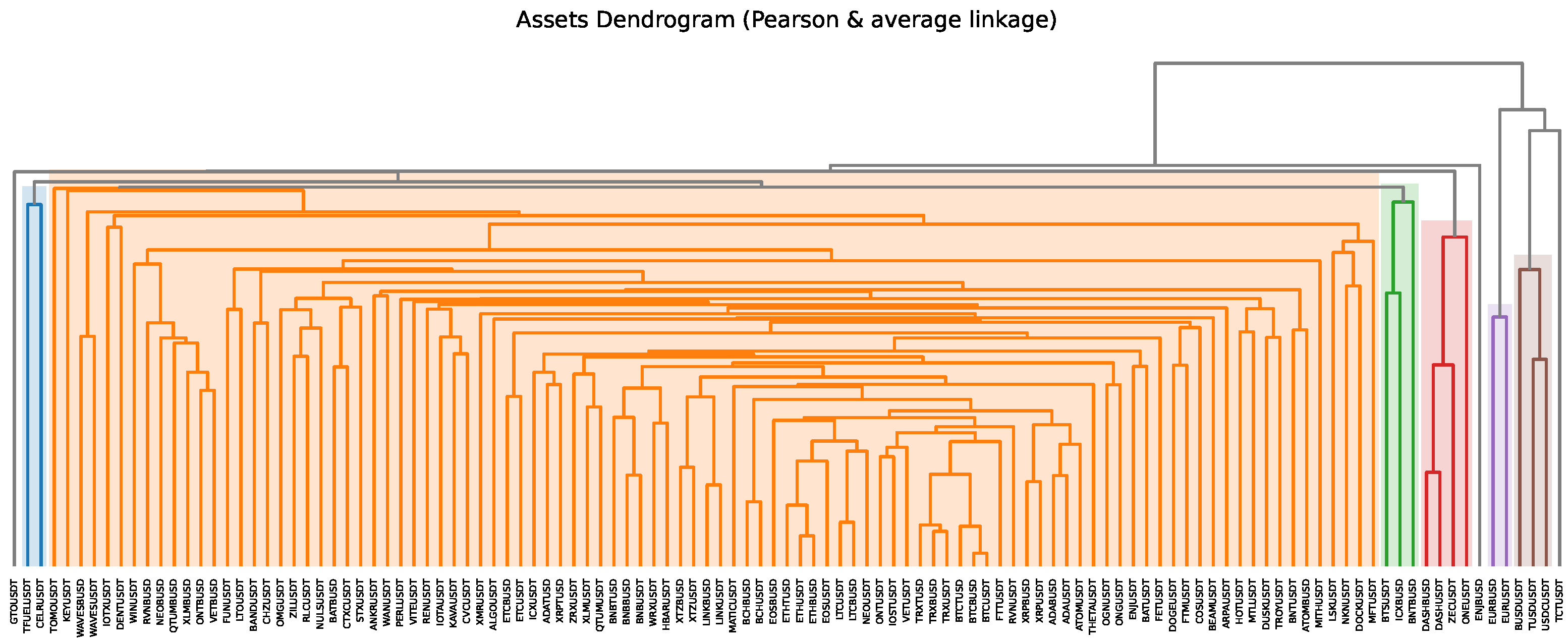
• 1. Computing the dendrogram using hierarchical tree clustering algorithm by using a distance matrix of the asset correlations.

  −

  First we compute the correlation among assets, which produces an $N\times N$ matrix we call $\rho$.

  −

  Then, we convert this to a distance matrix through

  $$D(i,j)=\sqrt{0.5\times (1-\rho (i,j\left)\right)}.$$

  −

  We next devise a new distance matrix $\widehat{D}$ which is actually a similarity matrix. It is computed as follows:

  $$\widehat{D}(i,j)=\sqrt{\sum _{k=1}^N{(D(k,i)-D(k,j))}^2}.$$

  −

  We then start to form clusters as follows:

  $$U=argmi{n}_{i,j}\widehat{D}(i,j).$$

  This gives us two indices $r_1$ and $c_1$, which are the row and column indices in $\widehat{D}$. We combine the assets given by the respective indices to obtain the first cluster $U\left[1\right]$. For more details on the procedure please see the original paper De Prado (2016).

  −

  We now delete the newly formed cluster assets row and column from the matrix ($r_1$ and $c_1$) and replace them with a single one. Computing distances between this new cluster and the remaining assets can be performed by multiple different criteria, as is the general case with clustering, either single-linkage, average-linkage, etc.

  −

  We repeat the last two steps until we have only one cluster. So we can see this is an agglomerative clustering algorithm. We show its dendrogram (graphical depiction of the hierarchical clustering) on our crypto data in Figure 2.

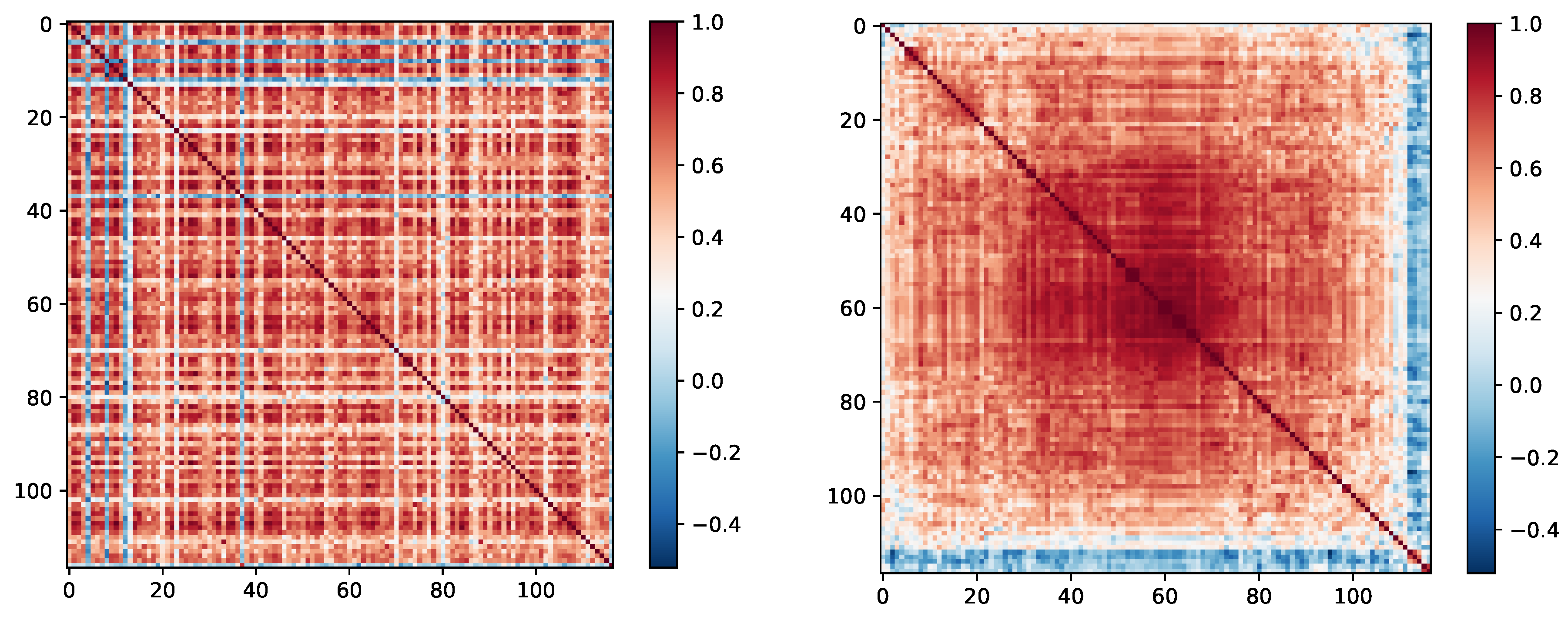
• 2. Doing matrix seriation. This procedure rearranges data in such a way that larger covariances are closer to the diagonal and that similar values are near. This results in a quasi-diagonal covariance matrix. We show this process on our own crypto dataset Figure 3.
• 3. Recursive bisection. This is the final step which actually assigns weights to the assets using the previous clustering. Looking at the hierarchical tree structure:

  −

  We first set all weights to 1.

  −

  Next, starting from the root, for each cluster we use the following weights to compute the volatilities:

  $$w_i=\frac{diag{\left(V_i\right)}^{-1}}{trace\left(diag{\left(V_i\right)}^{-1}\right)}.$$

  This uses the fact that for a diagonal covariance matrix, the inverse-variance allocations are optimal.

  −

  Then for the two branches of each node (a node corresponds to a cluster) we compute the variance: ${\sigma }_1=w_1^T{V}_1{w}_1$ and ${\sigma }_2=w_2^T{V}_2{w}_2$.

  −

  Finally, we rescale the weights as $w_i={\alpha }_i{w}_i$ with ${\alpha }_1=1-\frac{{\sigma }_1}{{\sigma }_1+{\sigma }_2}$ and ${\alpha }_2=1-{\alpha }_1$

Most HC models evaluated in the literature look at much larger time periods, and are often used for the analysis of the long-term asset behavior. We show that shorter periods can be used successfully and the overall system performance can be enhanced by adaptively selecting among them.

2.2. Deep Reinforcement Learning

In a different line of work, DRL has been applied with some degree of success in many markets Betancourt and Chen (2021); Jiang and Liang (2017); Zejnullahu et al. (2022); Zhang et al. (2020). One of the major differences between the two approaches, is the period at which they are evaluated on, with HRP and related approaches tackling much larger out-of-sample sets. Most DRL algorithms used in trading are generally trained for a long time and then their performance is evaluated for a short test time. This evaluation period needs to come immediately after the training period. The latter is thought to be required due to the nature of the market and the limitations of the agent which cannot generalize to many different dynamics. Another shortcoming of the DRL approach is that it generally requires a continuous action space, which is notoriously hard to explore.

The new DRL techniques applied on the portfolio management problem seemed to be reinventing the wheel, with some approaches even incorporating covariance estimation. Most of them used some of the existing theory but none of the existing practical models. The models coming from the financial community and DRL seemed to be mutually exclusive, despite tackling the same issue. You could either use one or the other. This is where we try to bridge the gap, by employing these more traditional HC models from the financial community, as a starting point and adding the DRL flexibility on top of them, we avoid its large computational requirements, large variance and instability. Our DRL works on a small number of state dimensions, the recent performance of all models. As for actions it selects among available models, 12 + 1 (hold) possible discrete actions.

In our work we overcome these limitations, leveraging a fast (much faster than DRL) and well-received algorithm (HRP) to be able to use a single agent without need for retraining and we use a discrete action space where each action corresponds to selecting one of the HRP and HERC models’ weights assignments.

2.3. Model-Based RL

Model-based RL assumes the existence of some abstract simulation of the world, either devised by the engineer, or learned by a machine learning algorithm. This simulation is then used to generate rewards and/or observations for the agent, which allows it to learn from experiences (which are now embedded in the simulation) without interacting with the real environment. Some advantages and constraints of having a model-based RL agent are:

• The interaction with the real environment might be risky, inducing large costs sometimes. Thus having a zero-cost alternative is desirable.
• Having an accurate enough model of the world is necessary for the agent to learn and behave well in the real environment.
• The model is not necessarily a perfect representation of the real world, but it is close enough to be useful.

There are not many published articles using model-based DRL on trading, but there are some: Wei et al. (2019); Yu et al. (2019). However, all of them deal with prediction of the future, and not with the actual trading. We incorporate in our system, a different type of model, a decision-making model, in which we already have a dozen working trading models which we then select from using our DRL agent. Moreover, since the market state is the same independent of the actions taken by the agent, we can compute the performance of many decision-making models in parallel.

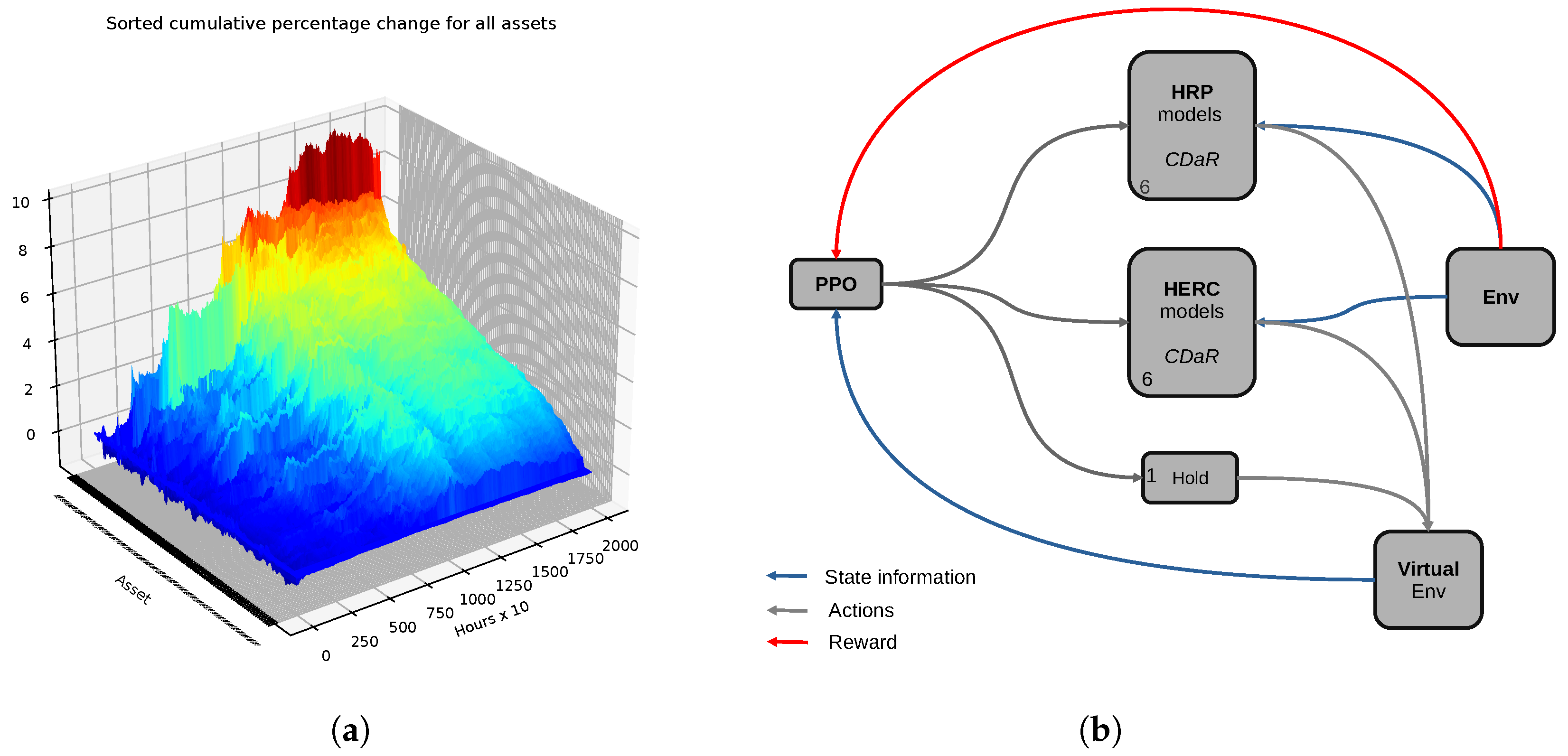
3. System Architecture

We use a high-level DRL agent (Proximal Policy Optimization Schulman et al. (2017)—PPO) which selects the next model to act on the market, based on its recent performance.

PPO is a policy optimization DRL algorithm which uses an approximation to a more analytical trust-region policy optimization Schulman et al. (2015). In general it has good properties throughout a range of tasks and reaches some solution in a reasonable amount of time. It is better behaved, in our experience, more stable than other DRL algorithms1.

We wanted to combine the flexibility of DRL with the efficiency and robustness of HC approaches. The motivation behind this is to harness the strengths of DRL, while overcoming its drawbacks: high-dimensional continuous action space, large state space and large variance in performance. The whole system is designed to adaptively deal with switching market regimes while avoiding the need for retraining, and it does so successfully as seen in the next section.

We first run the low-level models, the 12 HC models on the market to obtain their performance on the full dataset (Figure 4). We see that the performance is worse than the buy-and-hold strategy for most HC models. We save these models’ performances to a file (to avoid computing it every time they are requested by the DRL agent in the training phase) and load them up in each RL experiment. These performances of all models will function as state information for the DRL agent, indexed by the step we are at in the dataset. We also tried adding the returns of all assets, or using only the returns as a state but that produced a worse performance than just using the recent performance of all models.

By having multiple HRP and HERC models with different hyperparameters (see the whole set of hyperparameters in

Table 1. Hyperparameters for the HRP and HERC models.

Hyperparameter—Model	HRP	HERC
Risk measure	CDaR	CDaR
Codependence	Pearson	Pearson
Linkage	average	average
Max clusters	-	10
Optimal leaf order	True	True

, we vary the covariance estimation period, as it is significantly influencing performance), we ensure that our pool of decision making models is diverse. Thus, we account for different market regimes, and we remove the need for having the testing period right after the training period. This dependency on the recent past is now incorporated in the recent performance of the individual HC models (which is fed as a state to the PPO agent), thus allowing for much larger testing periods. We show good performance on the crypto market for as much as 13 months without any retraining (with training on 13 months as well). For details of the datasets used and train-test splits see

Table 2. Training and testing splits.

Market	Training Set	Testing Set
Crypto	22 March 2020 04:00–13 May 2021 14:00	13 May 2021 15:00–1 June 2022 03:00
Stocks	17 September 2019 15:30–16 December 2020 12:30	16 December 2020 13:30–4 February 2022 15:30
Forex	11 December 2020 01:00–30 September 2021 23:00	10 January 2021 00:00–28 September 2022 06:00

.

The data we chose were the most recent free data we found available at the time of the respective experiments. We tried to split the data similarly even if they had different sizes for each market, trying to keep a large testing set for each, to avoid cherry-picking, which can happen for small testing sets. We considered the fact that we ended up with different periods and different sizes for each market as beneficial for the overall robustness of sampling and evaluation of our system. The crypto data were taken from https://binance.com/ (accessed on 2 June 2022) through the python API, the forex data were taken from https://data.forexsb.com/ (accessed on 29 September 2022), while the stocks data were taken from https://www.alphavantage.co/ (accessed on 5 February 2022). The individual assets were selected based on how much valid data were available for each asset. We chose the assets with the fewest missing points. See the full list of assets in

Table 3. List of assets used on each market.

Cryptocurrencies		Stocks	Forex
ADABUSD	LINKBUSD	AAPL	AUDCAD
ADATUSD	LINKUSDT	ABT	AUDCHF
ADAUSDT	LSKUSDT	ACN	AUDJPY
ALGOUSDT	LTCBUSD	ADBE	AUDNZD
ANKRUSDT	LTCUSDT	AMD	AUDUSD
ARPAUSDT	LTOUSDT	AMZN	CADCHF
ATOMBUSD	MATICUSDT	ASML	CADJPY
ATOMUSDT	MFTUSDT	AVGO	CHFJPY
BANDUSDT	MITHUSDT	BABA	EURAUD
BATBUSD	MTLUSDT	BAC	EURCAD
BATUSDT	NEOBUSD	BHP	EURCHF
BCHBUSD	NEOUSDT	COST	EURGBP
BCHUSDT	NKNUSDT	CRM	EURJPY
BEAMUSDT	NULSUSDT	CSCO	EURNZD
BNBBUSD	OGNUSDT	CVX	EURUSD
BNBTUSD	OMGUSDT	DIS	GBPAUD
BNBUSDT	ONEUSDT	GOOG	GBPCAD
BNTBUSD	ONGUSDT	HD	GBPCHF
BNTUSDT	ONTBUSD	INTC	GBPJPY
BTCBUSD	ONTUSDT	JNJ	GBPNZD
BTCTUSD	PERLUSDT	JPM	GBPUSD
BTCUSDT	QTUMBUSD	KO	NZDCAD
BTSUSDT	QTUMUSDT	MA	NZDCHF
BUSDUSDT	RENUSDT	MCD	NZDJPY
CELRUSDT	RLCUSDT	MS	NZDUSD
CHZUSDT	RVNBUSD	MSFT	USDCAD
COSUSDT	RVNUSDT	NFLX	USDCHF
CTXCUSDT	STXUSDT	NKE	USDJPY
CVCUSDT	TCTUSDT	NVDA
DASHBUSD	TFUELUSDT	NVS
DASHUSDT	THETAUSDT	ORCL
DENTUSDT	TOMOUSDT	PEP
DOCKUSDT	TROYUSDT	PFE
DOGEUSDT	TRXBUSD	PG
DUSKUSDT	TRXTUSD	PM
ENJBUSD	TRXUSDT	QCOM
ENJUSDT	TUSDUSDT	TM
EOSBUSD	USDCUSDT	TMO
EOSUSDT	VETBUSD	TSLA
ETCBUSD	VETUSDT	TSM
ETCUSDT	VITEUSDT	UNH
ETHBUSD	WANUSDT	UPS
ETHTUSD	WAVESBUSD	V
ETHUSDT	WAVESUSDT	VZ
EURBUSD	WINUSDT	WMT
EURUSDT	WRXUSDT	XOM
FETUSDT	XLMBUSD
FTMUSDT	XLMUSDT
FTTUSDT	XMRUSDT
FUNUSDT	XRPBUSD
GTOUSDT	XRPTUSD
HBARUSDT	XRPUSDT
HOTUSDT	XTZBUSD
ICXBUSD	XTZUSDT
ICXUSDT	ZECUSDT
IOSTUSDT	ZILUSDT
IOTAUSDT	ZRXUSDT
IOTXUSDT	KEYUSDT
KAVAUSDT

.

Both the train and test periods start with an offset of 700 h, the maximum covariance estimation period among the HC decision making models. This means that no training or testing takes place in this interval.

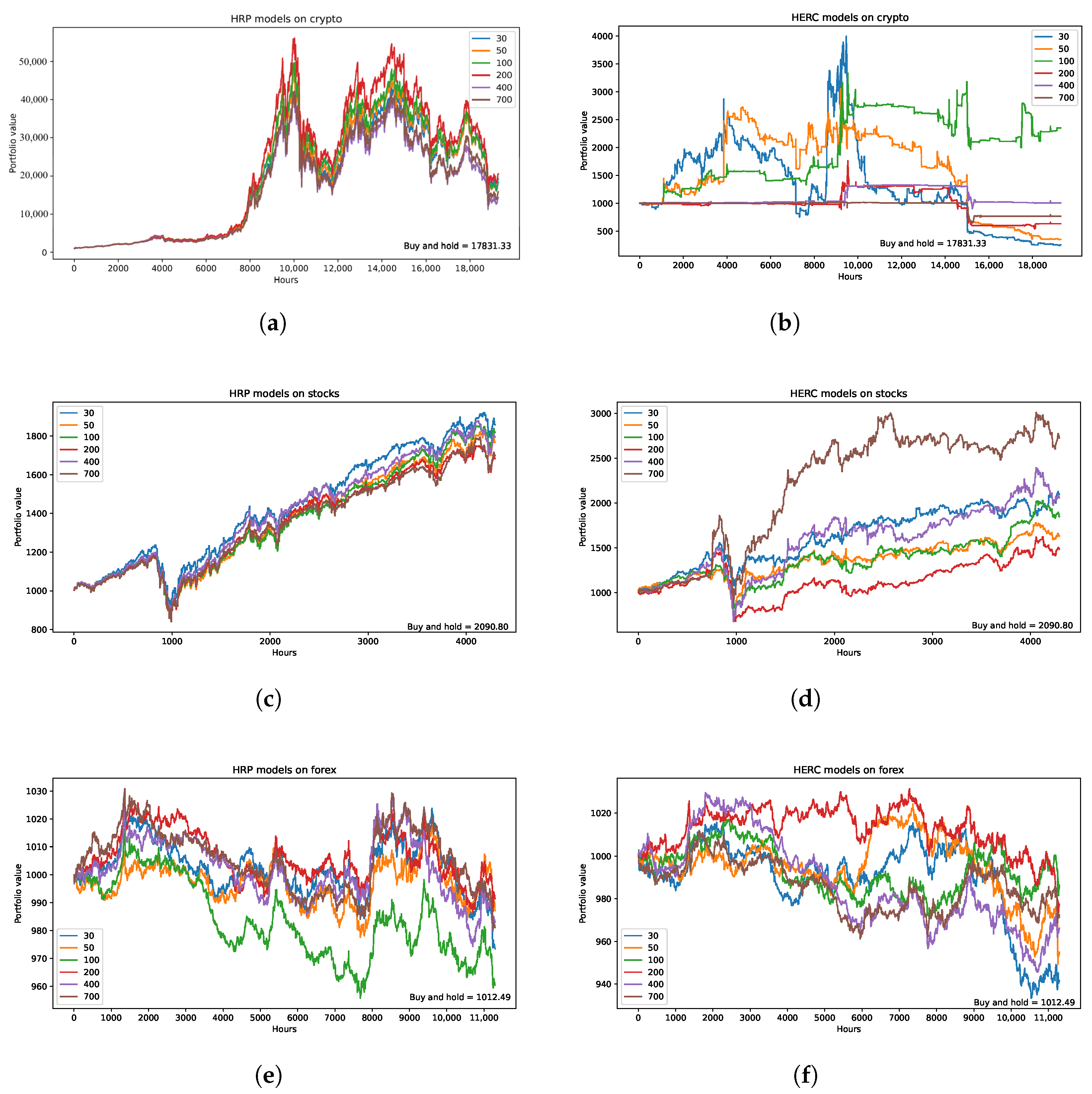
3.1. Performance of Individual HRP Models

We run multiple HRP models with different parameters in parallel since the problem setup allows this without any issues. See the results on the full datasets in Figure 4.

After we receive the prices for all assets for the current timestep, compute each model’s respective profits if allowed to trade on the real market. We assume there is some sort of smoothness in model performance, which recent history being indicative of the immediate future, so we are feeding the recent T steps of the model performance (actually its rate $\frac{P_t}{P_{t-1}}$, to make it independent of the value magnitude).

We use the riskfolio library2 to acquire the HRP and HERC solution, with the Conditional Drawdown at Risk (CDaR) as the risk measure to optimize the portfolio. CDaR is a measure similar to Conditional Variance at Risk (CVar, Uryasev (2000)), but which uses the drawdown instead of the variance of the assets. For more details on this measure see Goldberg and Mahmoud (2017).

In Figure 4 we show the performance of the individual HC models on all three markets. We vary the covariance estimation period, the parameter which influences significantly the portfolio selection at each step. HERC models are less correlated with other HERC models, with HRP models being highly correlated with other HRP models, however the HRP and HERC models are not correlated. The idea is to have more heterogeneous models such that the DRL agent can choose a better performing model when the performance of the current selection goes down.

In Figure 5 we can see the mean performance of the discrete DRL agent on each market (blue) with the black bars representing the sample standard deviation from 30 samples. We report the result of the best configuration of the hyperparameters. See

Table 4. Hyperparameters for the PPO model.

Hyperparameter—Model	PPO
Learning rate	grid_search([0.0001, 0.001, 0.01])
Value function clip	grid_search([1, 10, 100])
Gradient clip	grid_search([0.1, 1, 10])
Network	[1024, 512]
Activation function	ReLU
KL coeff	0.2
Clip parameter	0.3
Uses generalized advantage estimation	True

for the full list of hyperparameters used for PPO. The orange bars represent the performance of the continuous DRL agent, when we have 12 continuous actions, one value for each low-level agent. This should enable arbitrary policy learning, combining the best of each agent at each step, while still reducing the dimensionality of the action-space significantly. However, even if this showed better than random mean performance and much lower standard deviation (a much desired trait for a DRL agent), the performance was quite poor compared to the discrete agent. The green bars represent the performance of a random high-level policy, where only the DRL agent is replaced with a random policy, while the low-level agents remain the same. This is to directly compare the performance of a DRL policy with a random policy. The red bars represent a base policy which considers investing at the beginning of the evaluation period the same amount of cash (or USDT) in each of the available assets and holding them until the end of the evaluation period.

3.2. Rewards

For RL we used the RLlib library3. Aside from the classical reward given to a portfolio optimization agent, we add a hold reward, to incentivize the agent to hold when all the assets are going down. The reward at time t is given by:

$${\mathrm{reward}}_t=\sum _{i=1}^m{q}_t^i{p}_t^i-\sum _{i=1}^m{q}_{t-\tau }^i{p}_{t-\tau }^i$$

(1)

where $\tau$ is the number of low-level steps corresponding to a high-level step (we take this as 5), $q_t^i$ is the quantity of asset i at time t, $p_t^i$ is the price of asset i at time t, and $q_{t-1}^i$ is the quantity of asset i at time $t-1$. The quantity of asset i is always positive and is related to the weights $w_i^t$ of the portfolio at time t through the overall previous portfolio value, and is given by:

$$q_t^i=w_t^i·\frac{{\sum }_{j=1}^m{q}_{t-\tau }^j{p}_{t-\tau }^j}{p_{t-\tau }^i}$$

(2)

The reward for holding is given to the agent only when all assets have gone down and the recent action was hold. This is given by:

$${\mathrm{reward}}_{hold}=\sum _{i=1}^m\left(1-\frac{p_{t-\tau }^i}{p_t^i}\right)$$

(3)

3.3. Combining the Models

We can also combine the models weighted by some real value (so M continuous outputs, with M the number of models) which is the output of the DRL agent. The previous case is just a simplified version of this, where one of the outputs is 1 and the rest are all 0.

In this manner we can construct arbitrary policies, driven by the DRL agent. We can vary the discretization factor, allowing just a few discrete values for each model. This can be defined as d = how many values can the weight take between 0 and 1. If the answer is 2, we are in the previous case, where only one model acts at any point. However, if $d>2$ then we can have multiple models acting at the same time, with different weights. If d is ∞ then each weight is continuous. We test this version of the system as well, with a continuous-output DDPG Lillicrap et al. (2015) agent in place of the previous discrete-output PPO agent.

Despite training the DDPG agent for 10,000 iterations, it has not learned enough to produce any meaningful results. We omit the results, but we give the formulation here. The poor performance might be because of an insufficient hyperparameter search (see

Table 5. Hyperparameters for the DDPG model.

Hyperparameter—Model	DDPG
Actor learning rate	grid_search([1 $\times {10}^{-3}$, 1 $\times {10}^{-4}$, 1 $\times {10}^{-5}$])
Critic learning rate	grid_search([1 $\times {10}^{-3}$, 1 $\times {10}^{-4}$, 1 $\times {10}^{-5}$])
Network for actor and critic	[1024, 512]
Activation function	ReLU
Target network update frequency	grid_search([10, 100, 1000])

for hyperparameters used, and check the RLlib source for the full default set4).

We also tried a continuous version of the PPO agent, which shows marginally improved performance. Originally PPO was designed as a discrete action space algorithm, but in RLlib it can be used with continuous action spaces as well, by using a Gaussian distribution as the action distribution. We use the same hyperparameters as in the discrete case. Each model is given a weight $a_i$ (with i from 1 to M, in our case $M=12$) and the portfolio is constructed as follows. First we weigh the asset weights of the respective model by the model weight, which is one element of the output vector, or action, from the DDPG/PPO agent:

$$\overline{{\mathbf{w}}_i}=a_i·{\mathbf{w}}_i$$

(4)

Then we sum up to weights for each asset, for all models:

$${\overline{w}}^j=\sum _{i=1}^M{\overline{w}}_i^j\mathrm{for}j=1,\dots ,N\mathrm{where}N\mathrm{is}\mathrm{the}\mathrm{number}\mathrm{of}\mathrm{assets}$$

(5)

Finally, we normalize the weights to sum up to 1:

$${\widehat{w}}^j=\frac{{\overline{w}}^j}{{\sum }_{j=1}^N{\overline{w}}^j}$$

(6)

Normally, if the action components $a_i$ sum up to one then there is no need for the last normalization, however in RLlib they do have strange bounds sometimes.

4. Results

We show good performance on the crypto market for over a year without any retraining and in an extremely bear market. We start with an initial portfolio of USDT/USD 1000 and thus ending for example with USDT 2000 means we have gained $100\%$.

Since our base models are quite good already, it would be unfair to compare the results of our system (PPO + HC models) with a purely random policy. Thus we replace the PPO agent selecting among the HC models, with a random policy. We use this as a base-model comparison to our PPO agent.

We see in Figure 5 that the variances of both the PPO and random policies are similar for the crypto market (30 samples for each), and that the PPO agent clearly performs better than the random policy on all three markets.

We can attribute the large performance variance due to the fact that we are making decisions at a higher level, among models, and for multiple timesteps. The second baseline in Figure 5 is the buy-and-hold strategy for all assets. The strategy assumes an equal weight attribution for all assets. We see that a random policy at the high-level performs much better than the equal buy-and-hold strategy, at least for the crypto market.

We also see the different magnitudes of gains on different markets, with forex being the least profitable and having the smallest standard deviation. That is due to the nature of the time-series which has very low volatility compared to the crypto and stock market.

The performance is also clearly better than the individual HC models, which shows that our PPO agent managed to learn when to switch between models.

We chose such a large testing set to include both types of market conditions, bull and bear. However, to make sure we deal with widely different market conditions, we switch the training and testing sets. By doing so, we clearly brake the testing-after-training condition usually seen in the community. We show in Figure 6 the results on the stock and crypto markets for our system when the testing set is chronologically before the training set. In this case the crypto market has a very strong bull trend, but our system manages to obtain a significantly higher mean performance (30× vs. 50×). The y axis is on a logarithmic scale for better visualisation. In the stock market our system performs significantly better, even though the market trend is not strongly bullish.

5. Discussion

From evaluating our system without any retraining on large testing sets, which go through different regimes of the market, we can reliably say that our system works in more market conditions. Even seminal works such as Deng et al. (2016); Jiang et al. (2017) use a few very small isolated testing sets (50 days) with retraining in between. Some do use larger testing sets of 1–2 years, but with larger training sets (3 and up to 9 times) as well Li et al. (2019); Théate and Ernst (2021). Only in Zhang et al. (2020) we see truly large testing sets with a similar size as the training set, but on a different set of assets (a mix of futures), and they still use retraining. We also used different markets and different dataset sizes, adding to the robustness of the evaluation.

We thus add to the body of evidence that the market switches between different dynamics/regimes and having an explicit adaptive mechanism which deals with this switching is highly fruitful. A system with more decision-making layers can include additional useful information at selected layers, thus enabling structured processing of news data or macroeconomic indicators in a more meaningful way. The Ukraine–Russia conflict and the pandemic are such examples of macro-events which would clearly benefit a trading system if incorporated soundly.

6. Conclusions

We combined two of the newest and most performant ML techniques in a hierarchical decision-making system, with a DRL agent working as a high-level agent and selecting between a set of heterogeneous low-level HC agents to effectively act on the trading environment, i.e., assign weights to a portfolio of assets.

We showed that the DRL agent is able to learn when to switch between the low-level models, and that the performance is better than the individual models. We also showed that the performance is better than a random policy, which is a good baseline for the performance of the high level of decision making since the low levels supposedly have reasonable performance, thus a random high-level agent will surely perform better than a purely random agent.

Moreover, we were able to avoid retraining altogether, and increase the size of the testing set significantly, making it as large as the training set. All our results were obtained by using a default neural network with just two layers.

We also attempted to use a continuous action space for the DRL agent and combined ideal weights from each HC model, but this did not work well, or we were not able to find a good hyperparameter configuration for the DDPG agent.

Future work should try to find better hyperparameters, including the architecture of the network. One natural way to extend the current system is to add another level of decision-making and data aggregation, to deal with multiple markets in the same time. More data sources should also be useful, such as social media sentiments, and could be incorporated easily into the system, at selected levels.

The downside of an increasingly hierarchical system is the number of hyperparameters one has to choose from. The more individual agents, the more parameters we have, in addition to the ones used for their interaction. Joint training is prohibitive with a large number of levels, thus a mechanism for pretraining at each level is essential.

However, a hierarchical architecture shows the promise of having specialized and heterogeneous agents which can be selected alternatively to improve the overall system performance. Thus, a more thorough search for base models should be useful, with maybe some constraint which produces complementary models. Different decompositions of the strategy space should be also informative of the underlying market dynamics.

We devised a new architecture leveraging the flexibility of DRL and the reliability and efficiency of HC models. We avoided the notoriously hard to explore multi-dimensional action space generally used in the DRL trading literature, by having HC models which do the asset allocation and the DRL agent selects which seems to be the best one (based on recent performance) to act in the real environment. The applications are numerous, with the system being quite flexible and open to further research. One could use various different base models or use different reward functions (or combination thereof) for the DRL. One could even include a human in the loop as an additional low-level agent. Moreover, adding or removing assets does not require DRL retraining since the HC models deal with the actual asset allocation.

References

1. Betancourt, Carlos, and Wen-Hui Chen. 2021. Deep reinforcement learning for portfolio management of markets with a dynamic number of assets. Expert Systems with Applications 164: 114002. [Google Scholar] [CrossRef]
2. Black, Fischer, and Robert Litterman. 1992. Global portfolio optimization. Financial Analysts Journal 48: 28–43. [Google Scholar] [CrossRef]
3. Bodnar, Taras, Stepan Mazur, and Yarema Okhrin. 2017. Bayesian estimation of the global minimum variance portfolio. European Journal of Operational Research 256: 292–307. [Google Scholar] [CrossRef] [Green Version]
4. Burggraf, Tobias. 2021. Beyond risk parity—A machine learning-based hierarchical risk parity approach on cryptocurrencies. Finance Research Letters 38: 101523. [Google Scholar] [CrossRef]
5. Choueifaty, Yves, and Yves Coignard. 2008. Toward maximum diversification. The Journal of Portfolio Management 35: 40–51. [Google Scholar] [CrossRef] [Green Version]
6. Clarke, Roger, Harindra De Silva, and Steven Thorley. 2011. Minimum-variance portfolio composition. The Journal of Portfolio Management 37: 31–45. [Google Scholar] [CrossRef]
7. De Prado, Marcos Lopez. 2016. Building diversified portfolios that outperform out of sample. The Journal of Portfolio Management 42: 59–69. [Google Scholar] [CrossRef]
8. Deng, Yue, Feng Bao, Youyong Kong, Zhiquan Ren, and Qionghai Dai. 2016. Deep direct reinforcement learning for financial signal representation and trading. IEEE Transactions on Neural Networks and Learning Systems 28: 653–64. [Google Scholar] [CrossRef]
9. Goldberg, Lisa R., and Ola Mahmoud. 2017. Drawdown: From practice to theory and back again. Mathematics and Financial Economics 11: 275–97. [Google Scholar] [CrossRef] [Green Version]
10. Hirsa, Ali, Joerg Osterrieder, Branka Hadji-Misheva, and Jan-Alexander Posth. 2021. Deep reinforcement learning on a multi-asset environment for trading. arXiv arXiv:2106.08437. [Google Scholar] [CrossRef]
11. Jiang, Zhengyao, and Jinjun Liang. 2017. Cryptocurrency portfolio management with deep reinforcement learning. Paper presented at the 2017 Intelligent Systems Conference (IntelliSys), London, UK, September 7–8; pp. 905–13. [Google Scholar]
12. Jiang, Zhengyao, Dixing Xu, and Jinjun Liang. 2017. A deep reinforcement learning framework for the financial portfolio management problem. arXiv arXiv:1706.10059. [Google Scholar]
13. Jurczenko, Emmanuel. 2015. Risk-Based and Factor Investing. Amsterdam: Elsevier. [Google Scholar]
14. Kolm, Petter N., Reha Tütüncü, and Frank J. Fabozzi. 2014. 60 years of portfolio optimization: Practical challenges and current trends. European Journal of Operational Research 234: 356–71. [Google Scholar] [CrossRef]
15. Ledoit, Olivier, and Michael Wolf. 2003. Improved estimation of the covariance matrix of stock returns with an application to portfolio selection. Journal of Empirical Finance 10: 603–21. [Google Scholar] [CrossRef] [Green Version]
16. Li, Yang, Wanshan Zheng, and Zibin Zheng. 2019. Deep robust reinforcement learning for practical algorithmic trading. IEEE Access 7: 108014–22. [Google Scholar] [CrossRef]
17. Li, Yuxi. 2017. Deep reinforcement learning: An overview. arXiv arXiv:1701.07274. [Google Scholar]
18. Lillicrap, Timothy P., Jonathan J. Hunt, Alexander Pritzel, Nicolas Heess, Tom Erez, Yuval Tassa, David Silver, and Daan Wierstra. 2015. Continuous control with deep reinforcement learning. arXiv arXiv:1509.02971. [Google Scholar]
19. Maillard, Sébastien, Thierry Roncalli, and Jérôme Teïletche. 2010. The properties of equally weighted risk contribution portfolios. The Journal of Portfolio Management 36: 60–70. [Google Scholar] [CrossRef]
20. Markowitz, Harry M. 1952. Portfolio Selection. The Journal of Finance 7: 77–91. [Google Scholar]
21. Michaud, Richard O., and Robert Michaud. 2007. Estimation Error and Portfolio Optimization: A Resampling Solution. Available online: https://ssrn.com/abstract=2658657 (accessed on 20 September 2022).
22. Millea, Adrian. 2021. Deep reinforcement learning for trading—A critical survey. Data 6: 119. [Google Scholar] [CrossRef]
23. Mnih, Volodymyr, Koray Kavukcuoglu, David Silver, Andrei A. Rusu, Joel Veness, Marc G. Bellemare, Alex Graves, Martin Riedmiller, Andreas K. Fidjeland, Georg Ostrovski, and et al. 2015. Human-level control through deep reinforcement learning. Nature 518: 529–33. [Google Scholar] [CrossRef]
24. Moody, John, and Matthew Saffell. 1998. Reinforcement learning for trading. In Advances in Neural Information Processing Systems. Cambridge, MA: MIT Press, vol. 11. [Google Scholar]
25. Mosavi, Amirhosein, Yaser Faghan, Pedram Ghamisi, Puhong Duan, Sina Faizollahzadeh Ardabili, Ely Salwana, and Shahab S. Band. 2020. Comprehensive review of deep reinforcement learning methods and applications in economics. Mathematics 8: 1640. [Google Scholar] [CrossRef]
26. Raffinot, Thomas. 2017. Hierarchical clustering-based asset allocation. The Journal of Portfolio Management 44: 89–99. [Google Scholar] [CrossRef]
27. Raffinot, Thomas. 2018. The Hierarchical Equal Risk Contribution Portfolio. Available online: https://ssrn.com/abstract=3237540 (accessed on 20 September 2022).
28. Schulman, John, Filip Wolski, Prafulla Dhariwal, Alec Radford, and Oleg Klimov. 2017. Proximal policy optimization algorithms. arXiv arXiv:1707.06347. [Google Scholar]
29. Schulman, John, Sergey Levine, Pieter Abbeel, Michael Jordan, and Philipp Moritz. 2015. Trust region policy optimization. Paper presented at the International Conference on Machine Learning, Lille, France, July 6–11; pp. 1889–97. [Google Scholar]
30. Théate, Thibaut, and Damien Ernst. 2021. An application of deep reinforcement learning to algorithmic trading. Expert Systems with Applications 173: 114632. [Google Scholar]
31. Uryasev, Stanislav. 2000. Conditional value-at-risk: Optimization algorithms and applications. Paper presented at the IEEE/IAFE/INFORMS 2000 Conference on Computational Intelligence for Financial Engineering (CIFEr) (Cat. No. 00TH8520), New York, NY, USA, March 28; pp. 49–57. [Google Scholar]
32. Wei, Haoran, Yuanbo Wang, Lidia Mangu, and Keith Decker. 2019. Model-based reinforcement learning for predictions and control for limit order books. arXiv arXiv:1910.03743. [Google Scholar]
33. Yang, Hongyang, Xiao-Yang Liu, Shan Zhong, and Anwar Walid. 2020. Deep reinforcement learning for automated stock trading: An ensemble strategy. Paper presented at the First ACM International Conference on AI in Finance, New York, NY, USA, October 15–16; pp. 1–8. [Google Scholar]
34. Yu, Pengqian, Joon Sern Lee, Ilya Kulyatin, Zekun Shi, and Sakyasingha Dasgupta. 2019. Model-based deep reinforcement learning for dynamic portfolio optimization. arXiv arXiv:1901.08740. [Google Scholar]
35. Zejnullahu, Frensi, Maurice Moser, and Joerg Osterrieder. 2022. Applications of reinforcement learning in finance–trading with a double deep q-network. arXiv arXiv:2206.14267. [Google Scholar]
36. Zhang, Zihao, Stefan Zohren, and Stephen Roberts. 2020. Deep reinforcement learning for trading. The Journal of Financial Data Science 2: 25–40. [Google Scholar] [CrossRef]
Figure 1. Overview of the data (left) and system architecture (right). (a) Cumulative rate of change of all assets in the portfolio; (b) Overview of the system architecture.
Ijfs 11 00010 g001
Figure 2. Dendrogram of the hierarchical clustering of the crypto assets.
Ijfs 11 00010 g002
Figure 3. Original correlation distance matrix (left) and after matrix seriation or quasi-diagonalization (right).
Ijfs 11 00010 g003
Figure 4. Performance of individual HRP and HERC models. (a) HRP on crypto market (117 coins); (b) HERC on crypto market (117 coins); (c) HRP on stock market (46 stocks); (d) HERC on stock market (46 stocks); (e) HRP on forex (28 pairs); (f) HERC on forex (28 pairs).
Ijfs 11 00010 g004
Figure 5. Portfolio value by market.
Ijfs 11 00010 g005
Figure 6. Portfolio value by market.
Ijfs 11 00010 g006