Abstract
It has been argued in forensic science that the empirical validation of a forensic inference system or methodology should be performed by replicating the conditions of the case under investigation and using data relevant to the case. This study demonstrates that the above requirement for validation is also critical in forensic text comparison (FTC); otherwise, the trier-of-fact may be misled for their final decision. Two sets of simulated experiments are performed: one fulfilling the above validation requirement and the other overlooking it, using mismatch in topics as a case study. Likelihood ratios (LRs) are calculated via a Dirichlet-multinomial model, followed by logistic-regression calibration. The derived LRs are assessed by means of the log-likelihood-ratio cost, and they are visualized using Tippett plots. Following the experimental results, this paper also attempts to describe some of the essential research required in FTC by highlighting some central issues and challenges unique to textual evidence. Any deliberations on these issues and challenges will contribute to making a scientifically defensible and demonstrably reliable FTC available.
1. Introduction
1.1. Background and Aims
There is increasing agreement that a scientific approach to the analysis and interpretation of forensic evidence should consist of the following key elements (Meuwly et al. 2017; Morrison 2014, 2022):
- The use of quantitative measurements
- The use of statistical models
- The use of the likelihood-ratio (LR) framework
- Empirical validation of the method/system
These elements, it is argued, contribute towards the development of approaches that are transparent, reproducible, and intrinsically resistant to cognitive bias.
Forensic linguistic analysis (Coulthard and Johnson 2010; Coulthard et al. 2017) has been employed for analyzing documents as forensic evidence1 to infer the source of a questioned document (Grant 2007, 2010; McMenamin 2001, 2002). Indeed, this has been crucial in solving several cases; see e.g., Coulthard et al. (2017). However, analyses based on an expert linguist’s opinion have been criticized for lacking validation (Juola 2021). Even where textual evidence is measured quantitatively and analyzed statistically, the interpretation of the analysis has rarely been based on the LR framework (c.f., Ishihara 2017, 2021, 2023; Ishihara and Carne 2022; Nini 2023).
The lack of validation has been a serious drawback of forensic linguistic approaches to authorship attribution. However, there is a growing acknowledgment of the importance of validation in this field (Ainsworth and Juola 2019; Grant 2022; Juola 2021); This acknowledgment is fully endorsed. That being said, to the best of our knowledge, the community has not started thinking in depth as to what empirical validation obliges us to do. Looking at other areas of forensic science, there is already some degree of consensus on how empirical variation should be implemented (Forensic Science Regulator 2021; Morrison 2022; Morrison et al. 2021; President’s Council of Advisors on Science and Technology (U.S.) 2016). In forensic science more broadly, two main requirements2 for empirical validation are:
- Requirement 1: reflecting the conditions of the case under investigation;
- Requirement 2: using relevant data to the case.
The current study stresses that these requirements are also important in the analysis of forensic authorship evidence. This is demonstrated by comparing the results of the two competing types of experiments, one satisfying the above requirements and the other disregarding them.
The LR framework is employed in this study. LRs are calculated using a statistical model from the quantitatively measured properties of documents.
Real forensic texts have a mismatch or mismatches in topics, so this is the casework condition for which we will select relevant data. Amongst other factors, mismatch in topics is typically considered a challenging factor in authorship analysis (Kestemont et al. 2020; Kestemont et al. 2018). Cross-topic or cross-domain comparison is an adverse condition often used in the authorship attribution/verification challenges organized by PAN.3
Following the experimental results, this paper also describes future research necessary for forensic text comparison (FTC)4 by highlighting some crucial issues and challenges unique to the validation of textual evidence. These include (1) determining specific casework conditions and mismatch types that require validation; (2) determining what constitutes relevant data; and (3) the quality and quantity of data required for validation.
1.2. Likelihood-Ratio Framework
The LR framework has long been argued to be the logically and legally correct approach for evaluating forensic evidence (Aitken and Taroni 2004; Good 1991; Robertson et al. 2016) and it has received growing support from the relevant scientific and professional associations (Aitken et al. 2010; Association of Forensic Science Providers 2009; Ballantyne et al. 2017; Forensic Science Regulator 2021; Kafadar et al. 2019; Willis et al. 2015). In the United Kingdom, for instance, the LR framework will need to be deployed in all of the main forensic science disciplines by October 2026 (Forensic Science Regulator 2021).
An LR is a quantitative statement of the strength of evidence (Aitken et al. 2010), as expressed in Equation (1).
In Equation (1), the LR is equal to the probability () of the given evidence () assuming that the prosecution hypothesis () is true, divided by the probability of the same evidence assuming that the defense hypothesis () is true. The two probabilities can also be interpreted, respectively, as similarity (how similar the samples are) and typicality (how distinctive this similarity is). In the context of FTC, the typical is that “the source-questioned and source-known documents were produced by the same author” or “the defendant produced the source-questioned document”. The typical is that “the source-questioned and source-known documents were produced by different individuals” or “the defendant did not produce the source-questioned document”.
If the two probabilities are the same, then the LR = 1. If, however, is larger than , then the LR will be larger than one and this means that there is support for . If, instead, is larger than , then an LR < 1 will indicate that there is more support for (Evett et al. 2000; Robertson et al. 2016). The further away from one, the more strongly the LR supports either of the competing hypotheses. An LR of ten, for example, should be interpreted as the evidence being ten times more likely to be observed assuming the being true than assuming the being true.
The belief of the trier-of-fact regarding the hypotheses was possibly formed by previously presented evidence, and logically it should be updated by the LR. In a layperson’s term, that is, the belief of the decision maker regarding the suspect being guilty or not changes as a new piece of evidence is presented to them. This process is formally expressed in Equation (2).
Equation (2) is the so-called odds form of Bayes’ Theorem. It states that the multiplication of the prior odds and the LR equates to the posterior odds. The prior odds is the belief of the trier-of-fact with respect to the probability of the or being true, before the LR of a new piece of evidence is presented. The posterior odds quantifies the up-to-date belief of the trier-of-fact after the LR of the new evidence is presented.
As Equation (2) shows, calculation of the posterior odds requires both the prior odds and the LR. Thus, it is logically impossible for a forensic scientist to compute the posterior odds during their evidential analysis because they are not in the position of knowing the trier-of-fact’s belief. It is legally inappropriate for the forensic practitioner to present the posterior odds because the posterior odds concerns the ultimate issue of the suspect being guilty or not (Lynch and McNally 2003). If they do so, the forensic scientist deviates from their authority.
1.3. Complexity of Textual Evidence
Besides linguistic-communicative contents, various other pieces of information are encoded in texts. These may include information about (1) the authorship; (2) the social group or community the author belongs to; (3) the communicative situations under which the text was composed, and so on (McMenamin 2002). Every author or individual has their own ‘idiolect’: a distinctive individuating way of speaking and writing (McMenamin 2002). This concept of idiolect is fully compatible with modern theories of language processing in cognitive psychology and cognitive linguistics, as explained in Nini (2023).
The ‘group-level’ information that is associated with texts can be collated for the purpose of author profiling (Koppel et al. 2002; López-Monroy et al. 2015). The group-level information may include: the gender, age, ethnicity, and social-economical background of the author.
The writing style of each individual may vary depending on communicative situations that may be a function of internal and external factors. Some examples are the genre, topic, and level of formality of the texts; the emotional state of the author; and the recipient of the text.
As a result, a text is a reflection of the complex nature of human activities. As introduced in Section 1.1, we only focus on topic as a source of mismatch. However, topic is only one of many potential factors that influence individuals’ writing styles. Thus, in real casework, the mismatch between the documents under comparison is highly variable; consequently, it is highly case specific. This point is further discussed in Section 7.
2. Database and Setting up Mismatches in Topics
Taking up the problem of mismatched topics between the source-questioned and source-known documents as a case study, this study demonstrates that validation experiments should be performed by (1) reflecting the conditions of the case under investigation and (2) using data relevant to the case.
2.1. Database
The Amazon Authorship Verification Corpus (AAVC) http://bit.ly/1OjFRhJ (accessed on 30 September 2020) (Halvani et al. 2017) was used in this study. The AAVC contains reviews on Amazon products submitted by 3227 authors. As can be seen from Figure 1 which shows the number of reviews contributed by the authors, five or more reviews were collected from the majority of reviewers included in the AAVC. Altogether 21,347 reviews are included in the AAVC.
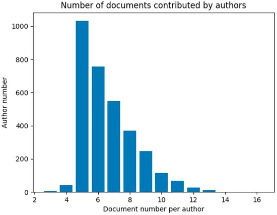
Figure 1.
Number of reviews (documents) contributed by authors.
The reviews are classified into 17 different categories as presented in Figure 2. In the AAVC, each review is equalized to 4 kB, which is approximately 700–800 words in length.
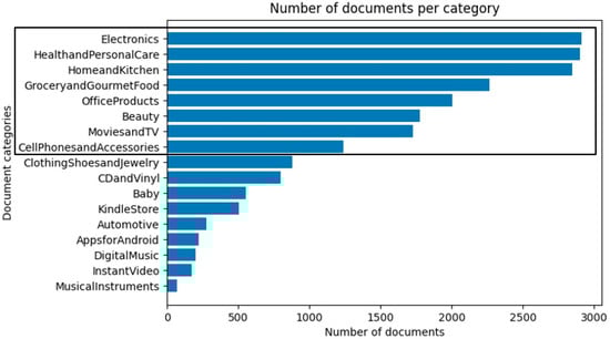
Figure 2.
The 17 review categories of the AAVC and their numbers of reviews. The categories that have the most reviews (top eight) are indicated by a black rectangle.
These reviews and the categories of the AAVC are referred to from now on as “documents” and “topics”, respectively.
The AAVC is a widely recognized corpus specifically designed for authorship verification studies, as evidenced by its utilization in various studies (Boenninghoff et al. 2019; Halvani et al. 2020; Ishihara 2023; Rivera-Soto et al. 2021). Certain aspects of the data, such as genre and document length, are well-controlled. However, there are uncontrolled variables that may bear relevance to the outcomes of the current study. For instance, there is no control over the input device used by reviewers (e.g., mobile device or computer) (Murthy et al. 2015), the English variety employed, or whether writing assistance functions such as automatic spelling and grammar checkers have been activated. All of these factors are likely to influence the writing style of individuals. Furthermore, the corpus may include some fake reviews, as the same user ID might be used by multiple reviewers, and conversely, the same reviewer may use multiple user IDs. Nonetheless, considering realistic forensic conditions, it is practically impossible to exert complete control over the data. Multiple corpora are often employed in authorship studies, investigating the robustness of systems across a variety of data. To the best of our knowledge, no peculiar behavior of the AAVC has been reported in any studies, ascertaining the quality of the corpus to the appropriate extent.
The topic categories employed in the AAVC appear to be somewhat arbitrary, with certain topics seemingly not situated at the same hierarchical level; for instance, “Cell Phones and Accessories” could be considered a subcategory of “Electronics”. Partially owing to overlaps across some topics, Section 2.2 will illustrate that documents belonging to certain topics exhibit similar patterns of distribution. Nevertheless, Section 2.2 also reveals that documents in some topics showcase unique distributional patterns distinct from other topics, and these topics are utilized for simulating topic mismatches.
2.2. Distributional Patterns of Documents Belonging to Different Topics
In order to show the similarities (or differences) between documents and topics, documents belonging to the top eight most frequent topics, which are indicated by a rectangle in Figure 2, are plotted in a two-dimensional space using t-distributed stochastic neighbor embedding (T-SNE)5 (van der Maaten and Hinton 2008) in Figure 3. Prior to the T-SNE, each document was vectorized via a transformer-based large language model, BERT6 (Devlin et al. 2019). Vectorization or word embedding is the process of converting texts to numerical vectors, which are high in dimension. In this way, each document is holistically represented in a semantically deep manner. Yet, it is difficult to visualize the high-dimensional data. T-SNE allows the visualization of high-dimensional data by reducing the dimension in a non-linear manner. T-SNE is a commonly used dimension reduction technique in which the text data are represented with word embeddings. This is because T-SNE is known to preserve the local and global relationships of data even after dimension reduction (van der Maaten and Hinton 2008). Thus, Figure 3 is considered to effectively depict the actual differences and similarities between the documents included in the different topics.
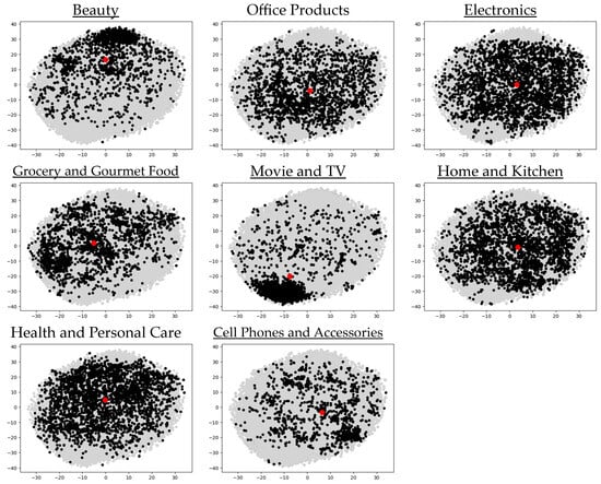
Figure 3.
T-SNE plots of the documents belonging to the eight topics indicated in Figure 2. The underlined topics are used for simulating the mismatches in topics. The red-filled circle in each plot shows the centroid of the documents belonging to the topic. x-axis = Dimension 1; y-axis = Dimension 2.
In Figure 3, each point represents a separate document. The distances between the points reflect the degrees of similarity or difference between the corresponding documents. Some topics have more points than others, reflecting the different numbers of documents included in the topics7 (see Figure 2). A red-filled circle in each plot indicates the centroid (the mean T-SNE values of Dimensions 1 and 2) of the documents belonging to the topic.
The documents belonging to the eight different topics display some unique distributional patterns; e.g., some topics show a similar distributional pattern to each other while other topics display their own unique patterns. The documents categorized into “Office Products”, “Electronics”, “Home and Kitchen”, and “Health and Personal Care” are similar to each other in that they are most widely distributed in the space; consequently, they extensively overlap each other. That is, there are a wide variety of documents included in these topics. The similarity of these four topics can also be seen from the fact that the centroids are all located in the middle of the plots. The documents in the “Beauty”, “Grocery and Gourmet Food”, “Movies and TV”, and “Cellphones and Accessories” topics are more locally distributed and their areas of concentrations are rather different. In particular, the documents in the “Beauty” and “Movie and TV” topics are most clustered in different areas; as a result, the centroids appear in different locations. That is, those documents belonging to each of the “Beauty” and “Movie and TV” topics are less diverse within each topic, but they are largely different from each other.
Primarily focusing on the overall distances between documents belonging to different topics, mismatches in topics were simulated in Section 2.3, varying in the degree of distance. Specifically, in these simulated mismatches, the degree of distance between the two centroids differs. Figure 3 illustrates that, in addition to the centroids’ locations, documents classified under different topics display diverse distributional patterns, with some being more dispersed or clustered than others. These distinctive distributional patterns may influence the experimental results, including LR values. However, the consideration of these patterns was limited primarily due to the difficulties associated with simulation.
2.3. Simulating Mismatch in Topics
Judging from the distributional patterns that can be observed from Figure 3 for the eight topics, the following three cross-topic settings were used for the experiments, together with paired documents that were randomly selected without considering their topic categories (Any-topics).
- Cross-topic 1: “Beauty” vs. “Movie and TV”
- Cross-topic 2: “Grocery and Gourmet Food” vs. “Cell Phones and Accessories”
- Cross-topic 3: “Home and Kitchen” vs. “Electronics”
- Any-topics: Any-topic vs. Any-topic
Cross-topics 1, 2, and 3 display different degrees of dissimilarity between the paired topics, which are visually observable in Figure 4.
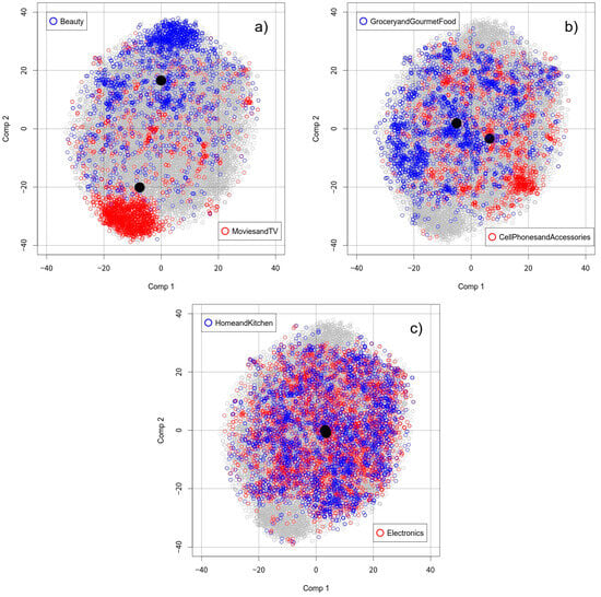
Figure 4.
Combined T-SNE plots for Cross-topics 1 (Panel a), 2 (Panel b), and 3 (Panel c), respectively. Black-filled circles in each panel show the centroids of the paired topics.
The documents classified as “Beauty” or “Movie and TV” (Cross-topic 1) show the greatest distances between the documents of the topics (see Figure 4a) in their distributions. The centroids of the documents for each topic, indicated by the black points, are far apart in Figure 4a. It can be foreseen that this large gap observed in Cross-topic 1 will make the FTC challenging. On the other hand, the documents classified as “Home and Kitchen” and “Electronics” (Cross-topic 3) heavily overlap each other in their distributions (see Figure 4c); the centroids are very closely located to each other, so it is likely that this FTC will be less challenging than for Cross-topic 1. Cross-topic 2 is somewhat in-between Cross-topic 1 and Cross-topic 3 in terms of the degree of overlap between the documents belonging to the “Grocery and Gourmet Food” and “Cell Phones and Accessories” topics.
The documents belonging to the “Any-topics” category were randomly selected from the AAVC.
Altogether, 1776 same-author (SA) and 1776 different-author (DA) pairs of documents were generated for each of the four settings given in the bullets above, and they were further partitioned into six mutually exclusive batches for cross-validation experiments. That is, 296 (=1776 ÷ 6) SA and 296 (=1776 ÷ 6) DA unique comparisons are included in each batch of the four settings. Refer to Section 3.1 for detailed information on data partitioning and the utilization of these batches in the experiments.
As can be seen from Figure 2, the number of documents included in each of the selected six topics is different; thus, the maximum numbers of paired documents for SA comparisons are also different between the three Cross-topics. The number of possible SA comparisons is 1776 for Cross-topic 2, and this is the smallest out of the three Cross-topics. Thus, the number of the SA comparisons is equalized to 1776 also for Cross-topics 1 and 3 by a random selection. The number of DA comparisons is also matched with that of SA comparisons. 1776 DA comparisons were randomly selected from all possible DA comparisons in such a way that each of the 1776 DA comparisons has a unique combination of authors.
Focusing on the mismatch in topics, two simulated experiments (Experiments 1 and 2) were prepared with the described subsets of the AAVC. Experiments 1 and 2 focus on Requirements 1 and 2, respectively. Experiments 1 and 2 each further include two types of experiments: one fulfilling the requirement and the other overlooking it. Detailed structures of the experiments will be described in Section 4.
3. Calculating Likelihood Ratios: Pipeline
After representing each document as a vector comprising a set of features, calculating an LR for a pair of documents under comparison (e.g., source-questioned and source-known documents) is a two-stage process consisting of the score-calculation stage and the calibration stage. The pipeline for calculating LRs is shown in Figure 5 for validation of the FTC system.
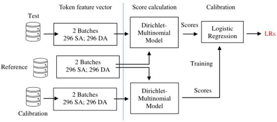
Figure 5.
Schematic illustration of the process for likelihood ratio calculations.
Details of the partitioned databases and the stages of the pipeline are provided in the following sub-sections.
3.1. Database Partitioning
As can be seen from Figure 5, three mutually exclusive databases are necessary for validating the performance of the LR-based FTC system. They are the Test, Reference, and Calibration databases. Using two independent batches (out of six) at a time for each of the Test, Reference, and Calibration databases, six cross-validation experiments are possible as shown in Table 1.

Table 1.
Use of the batches for the Test, Reference, and Calibration databases.
The SA and DA comparisons included in the Test database are used for assessing the performance of the FTC system. In the first stage of the pipeline given in Figure 5 (the score-calculation stage), a score is estimated for each comparison generated from the Test database, considering the similarity between the documents under comparison as well as the typicality of them. For assessing typicality, the necessary statistical information was obtained from the Reference database.
As two batches are used for each database in each of the six cross-validation experiments, 592 (=296 × 2) SA scores and 592 (=296 × 2) DA scores are obtained for each experiment. These 592 SA scores and 592 DA scores from the Test database are converted to LRs at the following stage of calibration. Scores are also calculated for the SA and DA comparisons from the Calibration database; that is, 592 SA and 592 DA scores for each experiment. These scores from the Calibration database are used to convert the scores of the Test database to LRs. For the explication of score calculation and calibration, see Section 3.3 and Section 3.4, respectively.
3.2. Tokenization and Representation
Each document was word-tokenized using the token() function of the quanteda R library (Benoit et al. 2018); the default settings were applied. Note that this tokenizer recognizes punctuation marks (e.g., ‘?’, ‘!’, and ‘.’) and special characters (e.g., ‘$’, ‘&’, and ‘%’) as independent words; thus, they constitute tokens by themselves. No stemming algorithm is applied. Upper and lower cases are treated separately; that is, ‘book’ and ‘Book’ are treated as separate words. It is known that the use of upper/lower case characters is fairly idiosyncratic (Zhang et al. 2014).
Each document of the AAVC is bag-of-words modelled with the 140 most frequent tokens appearing in the entire corpus, which are listed in Table A1 of Appendix A. The reader can verify that these are common words, being used regardless of topics. Obvious topic-specific words start appearing if the list of words is further extended.
An example the bag-of-words model is given in Example 1.
Example 1.
Document = .
The top 15 tokens are shown in Table 2 along with their occurrences. That is, these 15 tokens constitute the first 15 items of the bag-of-words feature vector: from to for Example 1. As could be expected, many of the tokens included in Table 2 are function words and punctuation marks.
Table 2.
Occurrences of the 15 most frequent tokens in the entire AAVC.
Many stylometric features have been developed to quantify writing style. Stamatatos (2009) classifies stylometric features into the five different categories of ‘lexical’, ‘character’, ‘syntactic’, ‘semantic’, and ‘application-specific’ and summarizes their pros and cons. It may be that different features have different degrees of tolerance to different types of mismatches. Thus, different features should be selectively used according to the casework conditions. However, it is not an easy task to unravel the relationships between them. Partly because of this, it is a common practice for the cross-domain authorship verification systems built on traditional feature engineering to use an ensemble of different feature types (Kestemont et al. 2020; Kestemont et al. 2021).
3.3. Score Calculation
The bag-of-words model consists of token counts, so the measured values are discrete. As such, the Dirichlet-multinomial statistical model was used to calculate scores. The effectiveness and appropriateness of the model for authorship-textual evidence has been demonstrated in Ishihara (2023). The formula for calculating a score for the source-questioned (X) and source-known (Y) documents with the Dirichlet-multinomial model is given in Equation (A1) of Appendix A. In essence, taking into account the discrete nature of the measured feature values, the model evaluates the similarity between X and Y and their typicality against the samples included in the Reference database, calculating a score. With the level of typicality held constant, the more similar X and Y are, the higher the score will be. Conversely, for an identical level of similarity, the more typical X and Y are, the smaller the score will become.
3.4. Calibration
The score obtained at the score-calculation stage for a pair of documents is LR-like in that it reveals the degree of similarity between the documents while considering the typicality with respect to the relevant population. However, if the Dirichlet-multinomial statistical model does not return well-calibrated outputs, they cannot be interpreted as LRs. In fact, this is often the case.8 This point is illustrated in Figure 6 using the distributions of imaginary SA and DA scores/LRs.
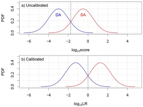
Figure 6.
Schematic illustration of the concept of calibration. SA and DA are the example outputs of a system for same-author and different-author comparisons, respectively; (a,b) are uncalibrated and calibrated systems, respectively. PDF—Probability density function.
In Figure 6a, the neutral point that optimally separates the DA and SA comparisons (the vertical dashed line of Figure 6a), is not aligned with a log10 value of 0, which is the neutral point in the LR framework. In such a case, the calculated value cannot be translated as the strength of the evidence. Thus, it is customarily called a ‘score’ (uncalibrated LR). Figure 6b is an example case of a calibrated system.
The scores (uncalibrated LRs) need to be calibrated or converted to LRs. Logistic regression is the standard method for this conversion (Morrison 2013). In other words, the scores of the Calibration database are used to train logistic regression for calibration.
Calibration is integral to the LR framework, as raw scores can be misleading until converted to LRs. Readers are encouraged to explore (Morrison 2013, 2018; Ramos and Gonzalez-Rodriguez 2013; Ramos et al. 2021) for a deeper understanding of the significance of calibration in evaluating evidential strength.
4. Experimental Design: Reflecting Casework Conditions and Using Relevant Data
Regarding the two requirements (Requirements 1 and 2) for validation stated in Section 1.1, two experiments (Experiments 1 and 2) were designed under cross-topic conditions. In the experiments, Cross-topic 1 is assumed to be the casework condition in which the source-questioned text is written on “Beauty” and the source-known text is written on “Movie and TV”. Readers will recall (Section 2.2) that Cross-topic 1 has a high degree of topic mismatch. In order to conduct validation under the casework conditions with the relevant data, the validation experiment should be performed with the databases having pairs of documents reflecting the same mismatch in topics as Cross-topic 1. Figure 7 elucidates this.
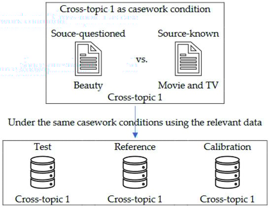
Figure 7.
Example illustrating validation under the same conditions as the casework with the relevant data.
Section 4.1 and Section 4.2 explain how Experiments 1 and 2 were set up, respectively. Experiment 1 considers Requirement 1 for validation, and Experiment 2 considers Requirement 2 for relevant data.
4.1. Experiment 1: Fulfilling or Not Fulfilling Casework Conditions
If the casework condition illustrated in Figure 7 were to be ignored, the validation experiment would be performed using Cross-topic 2, Cross-topic 3, or Any-topic. This is summarized in Table 3.
Table 3.
Conditions of Experiment 1.
The results of the validation experiments carried out under the conditions specified in Table 3 are presented and compared in Section 6.1.
4.2. Experiment 2: Using or Not Using Relevant Data
If data relevant to the case were not used for calculating the LR for the source-questioned and source-known documents under investigation, what would happen to the LR value? This question is the basis of Experiment 2. As such, in Experiment 2, validation experiments were carried out with the Reference and Calibration databases, which do not share the same type of topic mismatch as the Test database (Cross-topic 1). Table 4 includes the conditions used in Experiment 2.
Table 4.
Conditions of Experiment 2.
The results of the validation experiments carried out under the conditions specified in Table 4 are presented and compared in Section 6.2.
5. Assessment
The performance of a source-identification system is commonly assessed in terms of its identification accuracy and/or identification error rate. Metrics such as precision, recall, and equal error rate are typical in this context. However, these metrics are not appropriate for evaluating LR-based inference systems (Morrison 2011, p. 93). These metrics are based on the binary decision of whether the identification is correct or not, which is implicitly tied to the ultimate issue of the suspect being deemed guilty or not guilty. As explained in Section 1.2, forensic scientists should refrain from making references to this matter. Furthermore, these metrics fail to capture the gradient nature of LRs; they do not take into account the actual strength inherent in these ratios.
The performance of the FTC system was assessed by means of the log-likelihood-ratio cost (), which was first proposed by Brümmer and du Preez (2006). It serves as the conventional assessment metric for LR-based inference systems. The is described in detail in van Leeuwen and Brümmer (2007) and Ramos and Gonzalez-Rodriguez (2013). Equation (A2) of Appendix A is for calculating . An example of the calculation is also provided in Appendix A.
In the calculation of , each LR value attracts a certain cost.9 In general, the contrary-to-fact LRs; i.e., LR < 1 for SA comparisons and LR > 1 for DA comparisons, are assigned far more substantial costs than the consistent-with-fact LRs; i.e., LR > 1 for SA comparisons and LR < 1 for DA comparisons. For contrary-to-fact LRs, the cost increases as they are farther away from unity. For consistent-with-fact LRs, the cost increases as they become closer to unity. The is the overall average of the costs calculated for all LRs of a given experiment. See Appendix C.2 of Morrison et al. (2021) for the different cost functions of the consistent-with-fact and contrary-to-fact LRs.
The is a metric assessing the overall performance of an LR-based system. The consists of two metrics that assess the discrimination performance and calibration performance of the system, respectively. They are called discrimination loss () and calibration loss (). The is obtained by calculating the for the optimized LRs via the non-parametric pool-adjacent-violators algorithm. The difference between and is ; i.e., . If we consider the cases presented in Figure 6 as examples for , , and , the discriminating potential of the system in Figure 6a and that in Figure 6b are the same. In other words, the values for both are identical. The distinction lies in their values, where the value of Figure 6a should be higher than that of Figure 6b. Consequently, the overall will be higher for Figure 6a than for Figure 6b.
More detailed descriptions of these metrics can be found in Brümmer and du Preez (2006), Drygajlo et al. (2015) and in Meuwly et al. (2017).
A less than one means that the system provides useful information for discriminating between authors. The lower the value, therefore, the better the system performance. This holds true for both and , concerning the system’s discrimination and calibration performances.
The derived LRs are visualized by means of Tippett plots. A description of Tippett plots is given in Section 6.2., in which the LRs of some experiments are presented.
6. Results
The results of Experiments 1 and 2 are separately presented in Section 6.1 and Section 6.2. The reader is reminded that in each experiment, six cross-validated experiments were performed separately for each of the four conditions specified in Table 3 (Experiment 1) and Table 4 (Experiment 2), and also that Cross-topic 1, which has a large topic mismatch, is presumed to be the casework condition in which the source-questioned text is written on “Beauty” and the source-known text is written on “Movie and TV”.
6.1. Experiment 1
In Figure 8, the maximum, mean and minimum values of the six experiments are plotted for the four conditions given in Table 3. Please recall that the lower in , the better the performance.
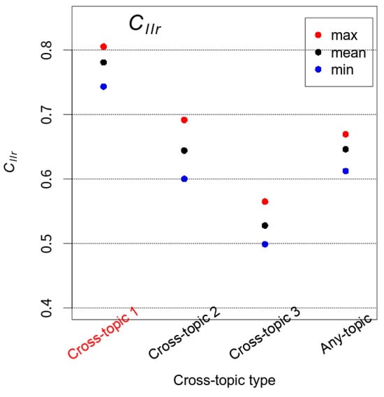
Figure 8.
The maximum (max), mean, and minimum (min) values of the six cross-validated experiments are plotted for each of the four experimental conditions specified in Table 3.
Regarding the degree of mismatch in topics that was described in Section 2.3, the experiment with Cross-topic 1, which matches the casework condition, yielded the worst performance result (mean = 0.78085) while the experiment with Cross-topic 3 yielded the best (mean = 0.52785). The experiments with Cross-topic 2 (mean = 0.65643) and Any-topic (mean = 0.64412) came somewhere in-between Cross-topics 1 and 3. It appears that the FTC system provides some useful information regardless of the experimental conditions; the values are all smaller than one. However, fact-finders would be led to believe that the performance of the FTC system is better than it actually is if they were informed with the validation result that does not match the casework condition; namely, Cross-topics 2 and 3 and Any-topic. Obviously, the opposite instance is equally likely in which an FTC system is judged to be worse than it actually is.
One may think it sensible to validate the system under less-constrained or more-inclusive heterogeneous conditions. However, the experimental result with Any-topic demonstrated that this was not appropriate, since the FTC system clearly performed differently from the experiment that was conducted under the same condition as the casework condition.
The performance of the FTC system is further analyzed by looking into its discrimination and calibration costs independently. The and are plotted one by one in Panels (a) and (b) of Figure 9 for the same experimental conditions listed in Table 3.
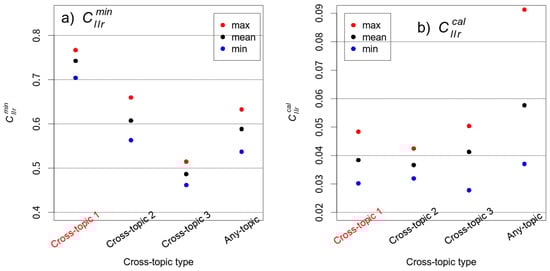
Figure 9.
The maximum (max), mean, and minimum (min) (Panel a) and (Panel b) values of the six cross-validated experiments are plotted for the four experimental conditions specified in Table 3.
The differences in discrimination performance (measured in ) observed in Figure 9a between the four conditions is parallel to the differences in overall performance (measured in ) observed in Figure 8 between the same four conditions. That is, the discrimination between the SA and DA documents is more challenging for one cross-topic type than another. The difficulty is in the descending order of Cross-topic 1, Cross-topic 2, and Cross-topic 3. The discrimination performance of Any-topic is marginally better than that of Cross-topic 2.
The values charted in Figure 9b are all close to zero and they are similar to each other; note that the range of the y-axis is very narrow between 0.02 and 0.09. That is to say, the resultant LRs are all well-calibrated. However, it appears that Any-topic (mean = 0.05766) underperforms the other Cross-topic types in calibration performance. The calibration performances of Cross-topics 1, 2 and 3 are virtually the same (mean is 0.03839 for Cross-topic 1; 0.03664 for Cross-topic 2; and 0.04126 for Cross-topic 3). As explained in Section 2.3, paired documents belonging to Any-topic were randomly selected from the entire database, which allows large variability between the batches. This could be a possible reason for the marginally larger values for Any-topic. However, this warrants further investigation.
6.2. Experiment 2
The maximum, mean and minimum values of the six experiments are plotted separately in Figure 10 for each of the four conditions specified in Table 4.
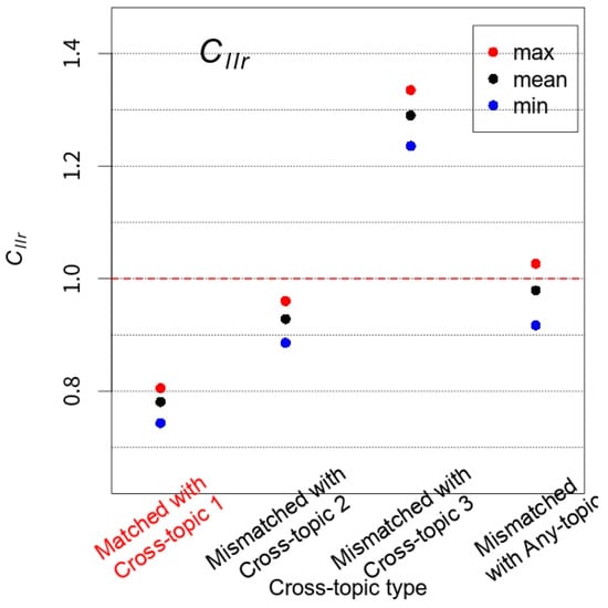
Figure 10.
The maximum (max), mean, and minimum (min) values of the six cross-validated experiments are plotted for each of the four experimental conditions specified in Table 4. The red horizontal-dashed line indicates .
The experimental results given in Figure 10 clearly show that it is detrimental to calculate LRs with data that is irrelevant to the case. The values can go beyond one, i.e., the system is not providing useful information for the case. The degree of deterioration in performance depends on the Cross-topic types used for Reference and Calibration databases. Cross-topic 3, which has the greatest difference from Cross-topic 1 (compare Figure 4a and Figure 4c), caused more substantial impediment in performance in comparison to Cross-topic 2. It is also interesting to see that the use of Any-topic for Reference and Calibration databases, which may be considered the most generic dataset reflecting the overall characteristics of the entire database, also brought about a decline in performance, as the values can go over one. The results included in Figure 10 well demonstrate the risk of using irrelevant data, i.e., the degree of topic mismatch is not comparable between Test and Reference/Calibration databases for calculating LRs. This may result in jeopardizing the genuine value of the evidence.
In order to further investigate the cause of the deterioration in overall performance (measured in ), the and are plotted in Figure 11 in the same manner as in Figure 9. Panels (a) and (b) are for the and , respectively.
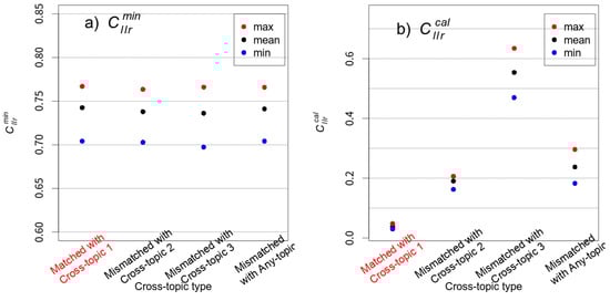
Figure 11.
The maximum (max), mean, and minimum (min) (Panel a) and (Panel b) values of the six cross-validated experiments are plotted for each of the four experimental conditions specified in Table 4.
Panel (a) of Figure 11 shows that the discrimination performance evaluated by is effectively the same across all of the experimental conditions ( mean: 0.74246 for Cross-topic 1; 0.73786 for Cross-topic 2; 0.73618 for Cross-topic 3; and 0.74102 for Any-topic). That is, as far as the discriminating power is concerned, the degree of mismatch in topics does not result in any sizable difference in discriminability. The discriminating power of the system remains unchanged before and after calibration, i.e., the value does not change before and after calibration. Since the Calibration database does not cause variability, and the Test database is fixed to Cross-topic 1, only the Reference database plays a role in the variability of the values across the four experimental conditions. The results given in Figure 11a imply that not using the relevant data for the Reference database does not have an apparently negative impact on the discriminability of the system. This point will be discussed further after the results of are presented below.
Panel (b) of Figure 11, which presents the values for the four experimental conditions, undoubtedly shows that not using the relevant data considerably impairs the calibration performance. It is interesting to see that the variability of the calibration performance is far smaller for the matched experiment (Cross-topic 1) than for the other mismatched experiments. Note that the maximum, mean, and minimum values are very close to each other for the matched experiment (Cross-topic 1). This means that the use of the relevant data is also beneficial in terms of the stability of the calibration performance.
The Tippett plots included in Figure 12 are for the LRs of the four experimental conditions described in Table 4. Note that the LRs of the six cross-validated experiments are pooled together for Figure 12. The deterioration in calibration described for Figure 11b can be visually observed from Figure 12.
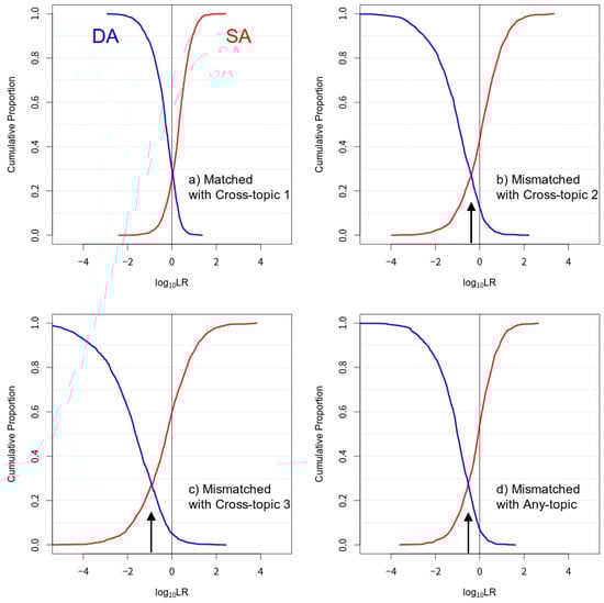
Figure 12.
Tippett plots of the LRs derived for the four experimental conditions specified in Table 4. Red curves—SA log10LRs; blue curves—DA log10LRs. Arrows indicate that the crossing-point of the two curves is not aligned with unity. Note that some log10LR values go beyond the range given in the x-axis.
Tippett plots, which are also called empirical cumulative probability distributions, show the magnitude of the derived LRs simultaneously for the same-source (e.g., SA) and different-source (e.g., DA) comparisons. In Tippett plots (see Figure 12), the y-axis values of the red curves give the proportion of SA comparisons with log10LR values smaller than or equal to the corresponding value on the x-axis. The y-axis values of the blue curves give the proportion of DA comparisons with log10LR values bigger than or equal to the corresponding value on the x-axis. Generally speaking, a Tippett plot in which the two curves are further apart and in which the crossing-point of the two curves is lower signifies a better performance. Provided that the system is well-calibrated, the LRs above the intersection of the two curves are consistent-with-fact LRs and the LRs below the intersection are contrary-to-fact LRs. In general, the greater the consistent-with-fact LRs are, the better, whereas the smaller the contrary-to-fact LRs are, the better.
The high values of the mismatched experiments with Cross-topic 2 (mean = 0.19037), Cross-topic 3 (mean = 0.55395), and Any-topic (mean = 0.23789) show that the resultant LRs are not well-calibrated. The crossing-points of the two curves given in Figure 12b–d, (see the arrows given in Figure 12) deviate from the neutral value of log10LR = 0, further demonstrating poor calibration.
The consistent-with-fact LRs are conservative in magnitude for the matched experiment with Cross-topic 1 (see Figure 12a), keeping the magnitude approximately within log10LR = ±3. The magnitude of the contrary-to-fact LRs is also constrained approximately within log10LR = ±2; this is a good outcome. In the mismatched experiments, although the magnitude of the consistent-with-fact LRs is greater than that of the matched experiment, the magnitude of the contrary-to-fact LRs is also unfavorably enhanced (see Figure 12b–d). That is, the LRs derived with irrelevant data (see Figure 12b–d) are at great risk of being overestimated. This overestimation can be exacerbated if the system is not calibrated (see Figure 12b–d).
Figure 11 indicates that the deterioration in overall performance (measured in ) is mainly due to the deterioration in calibration performance (measured in ), and that using irrelevant data, i.e., Cross-topics 2 and 3 and Any-topic in the Reference database, has minimal bearing on the discrimination performance.
Using simulated FTC data, Ishihara (2020) showed that performance degradation/deterioration caused by the limitation of available data was mainly attributed to poor calibration rather than to the poor discriminability potential; near-optimal discrimination performance can be achieved with samples from as few as 40–60 authors. Furthermore, in his forensic voice comparison (FVC) study investigating the impact of sample size on the performance of an FVC system, Hughes (2017) reported that the system performance was most sensitive to the number of speakers included in the Test and Calibration databases. The performance was not particularly influenced by the number of reference speakers. Although Ishihara’s and Hughes’ studies focus on the amount of data as a factor in the system performance, more specifically, the number of sources from which samples are collected, their results equally indicate that the calibration performance is more sensitive to the sample size than is the discrimination performance.
In the current study, the quantity of the data included in each database is sizable: 592 SA and 592 DA comparison for each experiment. Thus, unlike for Ishihara (2020) and Hughes (2017), the degraded aspect of data in the present study is not the quantity but the quality; namely, the degree of topic mismatch between Test and Reference/Calibration databases. It is conjectured that any adverse conditions in data, quantity, or quality, tend to do more harm on the calibration performance than the discrimination performance. However, this requires further investigation.
7. Summary and Discussion
Focusing on the mismatch in topics between the source-questioned and source-known documents, the present study showed how the trier-of-fact could be misled if the validation were NOT carried out:
- under conditions reflecting those of the case under investigation, and
- using data relevant to the case.
This study empirically demonstrated that the importance of the above requirements for validation is true for FTC.10
Although the necessity of validation for the admissibility of authorship evidence in court is well acknowledged in the community (Ainsworth and Juola 2019; Grant 2022; Juola 2021), to the best of our knowledge, the importance of the above requirements has never been explicitly stated in relevant authorship studies. This may be because it is rather obvious. However, we would like to emphasize the importance of the above validation requirements in this paper because forensic practitioners may think that they need to use heterogenous corpora in order to make up for the lack of specific corpora; for example, not having enough time to create a customized one, or thinking that the validation of any source-inference systems should be conducted by simultaneously covering a wide variety of conditions; for example, various types of mismatches should be considered. The inclusion of diverse conditions for validation is assumedly a legitimate way of understanding how well the system generally works. However, it does not necessarily mean that the same system works equally well for each specific situation; i.e., the unique condition of a given casework.
If one is working on a case in which the authorship of a given text is disputed and it is a hand-written text, the forensic expert would surely not use social media texts to validate the system with which the authorship analysis is performed. Likewise, they would not use the social media samples as the Reference and Calibration databases in order to calculate an LR for the hand-written text evidence. This analogy goes beyond the use of the same medium for validation and applies to various factors that influence one’s own way of writing.
This study focused on the mismatch in topics as a case study to demonstrate the importance of validation. Topic is a vague term, and the concept is not necessarily categorical; thus, it is a challenging task to classify documents into different topics/genres. One document may consist of multiple topics and each topic may be composed of multiple sub-topics. Making matters worse, as pointed out in Section 1.3, topic is only one of many other factors that possibly shape individuals’ writing styles. Thus, in real casework, the level of mismatch between the documents to be compared is highly variable and case specific, and databases replicating the case conditions may need to be built from scratch if suitable sources are not available. As such, it is sensible to ask what casework conditions need to be rigorously considered during validation and what other conditions can be overlooked, and these questions need to be pursued in the relevant academic community. These questions are inexorably related to the meaning of relevance. What are the relevant data (e.g., same/similar topics and medium) and relevant population (e.g., non-native use of a language; same assumed sex as the offender for some languages) (Hicks et al. 2017; Hughes and Foulkes 2015; Morrison et al. 2016)?
Computational authorship analysis has made huge progress over the last decade, and related work demonstrated that some sources of variability can be tolerated to a good extent by the systems compared to a decade ago. As the technology advances, fewer factors may become relevant to consider for validation. Authorship analysis can never be performed under perfectly controlled conditions because two documents are never composed under the exact same settings. Despite this inherent difficulty, authorship analysis has been successful. This leads to the conjecture that some external factors that are considered to be sources of variability can be well suppressed by the systems or that the magnitude of the impact caused by these factors may not be as substantial as feared in some cases.
Nevertheless, it is clear that the community of forensic authorship analysis needs to collaboratively attend to the issues surrounding validation, and to come up with a consensus, perhaps in the form of validation protocols or guidelines, regardless of the FTC approaches to be used. Although it is impossible to avoid some subjective judgement regarding the sufficiency of the reflectiveness of the casework conditions and the representativeness of the data relevant to the case (Morrison et al. 2021), validation guidelines and protocols should be prepared following the results of empirical studies. In fact, we are in a good position in this regard as there are already some guidelines and protocols for us to learn from; some of them are generic (Willis et al. 2015), and others are area-specific (Drygajlo et al. 2015; Morrison et al. 2021; Ramos et al. 2017) or approach-specific (Meuwly et al. 2017).
There are some possible ways of dealing with the issues surrounding the mismatches. One is to look for stylometric features that are robust to the mismatches (Halvani et al. 2020; Menon and Choi 2011), for example limiting the features to those that are claimed to be topic-agnostic (Halvani and Graner 2021; Halvani et al. 2020). Another is to build statistical models that can predict and compensate for the issues arising from the mismatches (Daumé 2009; Daumé and Marcu 2006; Kestemont et al. 2018).
Besides these approaches, an engineering approach is assumed to be possible; e.g., the relevant data are algorithmically selected and compiled considering the similarities to the source-questioned and source-known documents (Morrison et al. 2012) or they may even be synthesized using text-generation technologies (Brown et al. 2020). Nevertheless, these demand further empirical explorations.
The present study only considered one statistical model (Ishihara 2023) but there are other algorithms that might be more robust to mismatches, for example, methods designed for authorship verification that contain random variations in their algorithms (Kocher and Savoy 2017; Koppel and Schler 2004). Another avenue of future study is the application of a deep-learning approach to FTC. A preliminary LR-based FTC study using stylistic embedding reported promising results (Ishihara et al. 2022).
As briefly mentioned above, applying validation to FTC in a manner that reflects the casework conditions and uses relevant data most likely requires it to be performed independently for each case because each case is unique. This further necessitates custom-collected data for each casework. Given this need, unless an appropriate database already exists, the sample size—vis-à-vis both the length of a document and the number of authors documents are collected from—is an immediate issue as it is unlikely to be possible to collect an appropriate amount of data due to various constraints in a forensically realistic scenario. System performance is sensitive to insufficient data, in particular the number of sources from which samples are being collected, both in terms of its accuracy and reliability (Hughes 2017; Ishihara 2020). Thus, extended work is also required to assess the potential tradeoffs between the robustness of FTC systems and the data size,11 given the limitations of time and resources in FTC casework. Fully Bayesian methods whereby the LRs are subject to shrinkage depending on the degree of uncertainty (Brümmer and Swart 2014) would be a possible solution to the issues of sample size. That is, following Bayesian logic, the LR value should be closer to unity with smaller samples as the uncertainty will be higher.
8. Conclusions
This paper endeavored to demonstrate the application of validation procedures in FTC, in line with the general requirements stipulated in forensic science more broadly. By doing so, this study also highlighted some crucial issues and challenges unique to textual evidence while deliberating on some possible avenues for solutions to these. Any research on these issues and challenges will contribute to making a scientifically defensible and demonstrably reliable FTC method available. This will further enable forensic scientists to perform the analysis of text evidence accurately, reliably, and in a legally admissible manner, while improving the transparency and efficacy of legal proceedings. For this, we need to capitalize on the accumulated knowledge and skills in both forensic science and forensic linguistics.
Author Contributions
Conceptualization, S.I., S.K., M.C., S.E. and A.N.; methodology, S.I., S.K., M.C., S.E. and A.N.; software, S.I. and S.K.; validation, S.I. and S.K.; formal analysis, S.I. and S.K.; investigation, S.I., S.K., M.C., S.E. and A.N.; resources, S.I., S.K. and M.C.; data curation, S.I. and S.K.; writing—original draft preparation, S.I.; writing—review and editing, S.I., S.K., M.C., S.E. and A.N.; visualization, S.I. and S.K.; supervision, S.I.; project administration, S.I.; funding acquisition, S.I., S.K. and M.C. All authors have read and agreed to the published version of the manuscript.
Funding
The contributions from Shunichi Ishihara, Sonia Kulkarni, and Michael Carne were partially supported by an anonymous institution that prefers not to disclose its identity.
Data Availability Statement
The numerical version of the data and the codes (R/Python) used in this study are available from the corresponding author.
Acknowledgments
The authors thank the reviewers for their useful comments.
Conflicts of Interest
The authors declare no conflicts of interest.
Appendix A
Table A1.
The 140 tokens used for the bag-of-words model.
Table A1.
The 140 tokens used for the bag-of-words model.
| . | the | “ (open) | ” (close) | I | and | a |
| to | it | of | is | for | that | in |
| this | you | with | my | on | have | but |
| n't | 's | not | are | was | as | The |
| ) | be | It | ( | so | or | like |
| ! | one | do | can | they | use | very |
| at | just | all | This | out | has | up |
| from | would | more | good | your | if | an |
| me | when | ' ' | these | had | them | will |
| `` | than | about | get | great | does | well |
| really | product | which | other | some | did | no |
| time | - | much | 've | only | also | little |
| : | 'm | because | there | used | by | what |
| too | been | any | even | easy | using | am |
| … | were | we | better | could | work | after |
| into | nice | first | make | over | off | love |
| need | They | how | still | two | think | ? |
| then | If | price | way | bit | My | who |
| back | want | their | quality | most | works | made |
| find | years | see | few | enough | long | now |
The formula for calculating a score for the source-questioned () and source-known () documents with the Dirichlet-multinomial model is given in Equation (A1), in which is a multinomial beta function and is a parameter set for the Dirichlet distribution. The index is 140.
The parameters of the Dirichlet model () were estimated using the Reference database with the maximum likelihood estimation. A derivational process from Equation (1) to Equation (A1) is explicated in Ishihara (2023).
Equation (A2) is for calculating .
In Equation (A2), and are the linear LR values corresponding to SA and DA comparisons, respectively, and and are the numbers of the SA and DA comparisons, respectively.
For example, linear LR values of 10 and 100 for DA comparisons are contrary-to-fact LR values. The latter strongly supports the contrary hypothesis more than the former; thus, the latter should be more severely penalized than the former in terms of . In fact, the cost for the latter, 6.65821 (), is higher than that for the former, 3.4534 ().
Notes
| 1 | There are various types of forensic evidence, such as DNA, fingerprints, and voice analysis. The corresponding verification systems demonstrate varying degrees of accuracy for each. Authorship evidence is likely to be considered less accurate compared to other types within the biometric menagerie (Doddington et al. 1998; Yager and Dunstone 2008). |
| 2 | There is an argument suggesting that these requirements may not be uniformly applicable to all forensic-analysis methods with equal success (Kirchhüebel et al. 2023). It is proposed that a customized approach to method validation is necessary, contingent upon the specific analysis methods. |
| 3 | https://pan.webis.de/clef19/pan19-web/authorship-attribution.html (accessed on 3 February 2021). |
| 4 | Instead of more common terms such as ‘forensic authorship attribution’, ‘forensic authorship verification’, and ‘forensic authorship analysis’, the term ‘forensic text comparison’ is used in this study. This is to emphasize that the task of the forensic scientist is to compare the texts concerned and calculate an LR for them in order to assist the trier-of-fact’s decision on the case. |
| 5 | T-SNE is a statistical method for mapping high-dimensional data to a two- or three-dimensional space. It was performed with the T-SNE function of Python ‘sklearn’ library with ‘random_state = 123’ and ‘perplexity = 50’. |
| 6 | More specifically ‘bert-base-uncased’ was used as the pre-trained model with ‘max_position_embedding = 1024’; ‘max_length = 1024’; and ‘padding = max_length’. |
| 7 | T-SNE is non-deterministic. Therefore, the T-SNE plots were generated multiple times, both with and without normalizing the document number. However, the result is essentially the same regardless of the normalization. |
| 8 | If the output of the Dirichlet-multinomial system is well-calibrated, it is an LR, not a score. Thus, it does not need to be converted to an LR at the calibration stage. |
| 9 | This is true as long as the LR is greater than zero and smaller than infinity. |
| 10 | It is important to note that the present paper covers only the validation of FTC systems or systems based on quantitative measurements. There are other forms of validation when not quantifying features (Mayring 2020). |
| 11 | Some authors of the present paper, who are also FTC caseworkers, are often given a large amount of texts written by the defendant for FTC analyses. Thus, the amount of data in today’s cases could be huge, leading to the opposite problem of having too much data. However, when it comes to the data for the use of validation, e.g., Test, Reference, and Calibration data, it could still be a challenging task to collect an adequate amount of data from a sufficient number of authors. |
References
- Ainsworth, Janet, and Patrick Juola. 2019. Who wrote this: Modern forensic authorship analysis as a model for valid forensic science. Washington University Law Review 96: 1159–89. [Google Scholar]
- Aitken, Colin, and Franco Taroni. 2004. Statistics and the Evaluation of Evidence for Forensic Scientists, 2nd ed. Chichester: John Wiley & Sons. [Google Scholar]
- Aitken, Colin, Paul Roberts, and Graham Jackson. 2010. Fundamentals of Probability and Statistical Evidence in Criminal Proceedings: Guidance for Judges, Lawyers, Forensic Scientists and Expert Witnesses. London: Royal Statistical Society. Available online: http://www.rss.org.uk/Images/PDF/influencing-change/rss-fundamentals-probability-statistical-evidence.pdf (accessed on 4 July 2011).
- Association of Forensic Science Providers. 2009. Standards for the formulation of evaluative forensic science expert opinion. Science & Justice 49: 161–64. [Google Scholar] [CrossRef]
- Ballantyne, Kaye, Joanna Bunford, Bryan Found, David Neville, Duncan Taylor, Gerhard Wevers, and Dean Catoggio. 2017. An Introductory Guide to Evaluative Reporting. Available online: https://www.anzpaa.org.au/forensic-science/our-work/projects/evaluative-reporting (accessed on 26 January 2022).
- Benoit, Kenneth, Kohei Watanabe, Haiyan Wang, Paul Nulty, Adam Obeng, Stefan Müller, and Akitaka Matsuo. 2018. quanteda: An R package for the quantitative analysis of textual data. Journal of Open Source Software 3: 774. [Google Scholar] [CrossRef]
- Boenninghoff, Benedikt, Steffen Hessler, Dorothea Kolossa, and Robert Nickel. 2019. Explainable authorship verification in social media via attention-based similarity learning. Paper presented at 2019 IEEE International Conference on Big Data, Los Angeles, CA, USA, December 9–12. [Google Scholar]
- Brown, Tom, Benjamin Mann, Nick Ryder, Melanie Subbiah, Jared D Kaplan, Prafulla Dhariwal, Arvind Neelakantan, Pranav Shyam, Girish Sastry, Amanda Askell, and et al. 2020. Language models are few-shot learners. Advances in Neural Information Processing Systems 33: 1877–901. [Google Scholar]
- Brümmer, Niko, and Albert Swart. 2014. Bayesian calibration for forensic evidence reporting. Paper presented at Interspeech 2014, Singapore, September 14–18. [Google Scholar]
- Brümmer, Niko, and Johan du Preez. 2006. Application-independent evaluation of speaker detection. Computer Speech and Language 20: 230–75. [Google Scholar] [CrossRef]
- Coulthard, Malcolm, Alison Johnson, and David Wright. 2017. An Introduction to Forensic Linguistics: Language in Evidence, 2nd ed. Abingdon and Oxon: Routledge. [Google Scholar]
- Coulthard, Malcolm, and Alison Johnson. 2010. The Routledge Handbook of Forensic Linguistics. Milton Park, Abingdon and Oxon: Routledge. [Google Scholar]
- Daumé, Hal, III. 2009. Frustratingly easy domain adaptation. arXiv arXiv:0907.1815. [Google Scholar] [CrossRef]
- Daumé, Hal, III, and Daniel Marcu. 2006. Domain adaptation for statistical classifiers. Journal of Artificial Intelligence Research 26: 101–26. [Google Scholar] [CrossRef]
- Devlin, Jacob, Ming-Wei Chang, Kenton Lee, and Kristina Toutanova. 2019. BERT: Pre-training of deep bidirectional transformers for language understanding. Paper presented at 17th Annual Conference of the North American Chapter of the Association for Computational Linguistics: Human Language Technologies, Minneapolis, MN, USA, June 9–12. [Google Scholar]
- Doddington, George, Walter Liggett, Alvin Martin, Mark Przybocki, and Douglas Reynolds. 1998. SHEEP, GOATS, LAMBS and WOLVES: A statistical analysis of speaker performance in the NIST 1998 speaker recognition evaluation. Paper presented at the 5th International Conference on Spoken Language Processing, Sydney, Australia, November 30–December 4. [Google Scholar]
- Drygajlo, Andrzej, Michael Jessen, Sefan Gfroerer, Isolde Wagner, Jos Vermeulen, and Tuija Niemi. 2015. Methodological Guidelines for Best Practice in Forensic Semiautomatic and Automatic Speaker Recognition (3866764421). Available online: http://enfsi.eu/wp-content/uploads/2016/09/guidelines_fasr_and_fsasr_0.pdf (accessed on 28 December 2016).
- Evett, Ian, Graham Jackson, J. A. Lambert, and S. McCrossan. 2000. The impact of the principles of evidence interpretation on the structure and content of statements. Science & Justice 40: 233–39. [Google Scholar] [CrossRef]
- Forensic Science Regulator. 2021. Forensic Science Regulator Codes of Practice and Conduct Development of Evaluative Opinions. Available online: https://assets.publishing.service.gov.uk/government/uploads/system/uploads/attachment_data/file/960051/FSR-C-118_Interpretation_Appendix_Issue_1__002_.pdf (accessed on 18 March 2022).
- Good, Irving. 1991. Weight of evidence and the Bayesian likelihood ratio. In The Use of Statistics in Forensic Science. Edited by Colin Aitken and David Stoney. Chichester: Ellis Horwood, pp. 85–106. [Google Scholar]
- Grant, Tim. 2007. Quantifying evidence in forensic authorship analysis. International Journal of Speech, Language and the Law 14: 1–25. [Google Scholar] [CrossRef]
- Grant, Tim. 2010. Text messaging forensics: Txt 4n6: Idiolect free authorship analysis? In The Routledge Handbook of Forensic Linguistics. Edited by Malcolm Coulthard and Alison Johnso. Milton Park, Abingdon and Oxon: Routledge, pp. 508–22. [Google Scholar]
- Grant, Tim. 2022. The Idea of Progress in Forensic Authorship Analysis. Cambridge: Cambridge University Press. [Google Scholar]
- Halvani, Oren, and Lukas Graner. 2021. POSNoise: An effective countermeasure against topic biases in authorship analysis. Paper presented at the 16th International Conference on Availability, Reliability and Security, Vienna, Austria, August 17–20. [Google Scholar]
- Halvani, Oren, Christian Winter, and Lukas Graner. 2017. Authorship verification based on compression-models. arXiv arXiv:1706.00516. [Google Scholar] [CrossRef]
- Halvani, Oren, Lukas Graner, and Roey Regev. 2020. Cross-Domain Authorship Verification Based on Topic Agnostic Features. Paper presented at CLEF (Working Notes), Thessa-loniki, Greece, September 22–25. [Google Scholar]
- Hicks, Tacha, Alex Biedermann, Jan de Koeijer, Franco Taroni, Christophe Champod, and Ian Evett. 2017. Reply to Morrison et al. (2016) Refining the relevant population in forensic voice comparison—A response to Hicks et al. ii (2015) The importance of distinguishing information from evidence/observations when formulating propositions. Science & Justice 57: 401–2. [Google Scholar] [CrossRef]
- Hughes, Vincent. 2017. Sample size and the multivariate kernel density likelihood ratio: How many speakers are enough? Speech Communication 94: 15–29. [Google Scholar] [CrossRef]
- Hughes, Vincent, and Paul Foulkes. 2015. The relevant population in forensic voice comparison: Effects of varying delimitations of social class and age. Speech Communication 66: 218–30. [Google Scholar] [CrossRef]
- Ishihara, Shunichi. 2017. Strength of linguistic text evidence: A fused forensic text comparison system. Forensic Science International 278: 184–97. [Google Scholar] [CrossRef] [PubMed]
- Ishihara, Shunichi. 2020. The influence of background data size on the performance of a score-based likelihood ratio system: A case of forensic text comparison. Paper presented at the 18th Workshop of the Australasian Language Technology Association, Online, January 14–15. [Google Scholar]
- Ishihara, Shunichi. 2021. Score-based likelihood ratios for linguistic text evidence with a bag-of-words model. Forensic Science International 327: 110980. [Google Scholar] [CrossRef] [PubMed]
- Ishihara, Shunichi. 2023. Weight of Authorship Evidence with Multiple Categories of Stylometric Features: A Multinomial-Based Discrete Model. Science & Justice 63: 181–99. [Google Scholar] [CrossRef]
- Ishihara, Shunichi, and Michael Carne. 2022. Likelihood ratio estimation for authorship text evidence: An empirical comparison of score- and feature-based methods. Forensic Science International 334: 111268. [Google Scholar] [CrossRef] [PubMed]
- Ishihara, Shunichi, Satoru Tsuge, Mitsuyuki Inaba, and Wataru Zaitsu. 2022. Estimating the strength of authorship evidence with a deep-learning-based approach. Paper presented at the 20th Annual Workshop of the Australasian Language Technology Association, Adelaide, Australia, December 14–16. [Google Scholar]
- Juola, Patrick. 2021. Verifying authorship for forensic purposes: A computational protocol and its validation. Forensic Science International 325: 110824. [Google Scholar] [CrossRef]
- Kafadar, Karen, Hal Stern, Maria Cuellar, James Curran, Mark Lancaster, Cedric Neumann, Christopher Saunders, Bruce Weir, and Sandy Zabell. 2019. American Statistical Association Position on Statistical Statements for Forensic Evidence. Available online: https://www.amstat.org/asa/files/pdfs/POL-ForensicScience.pdf (accessed on 5 May 2022).
- Kestemont, Mike, Enrique Manjavacas, Ilia Markov, Janek Bevendorff, Matti Wiegmann, Efstathios Stamatatos, Martin Potthast, and Benno Stein. 2020. Overview of the cross-domain authorship verification task at PAN 2020. Paper presented at the CLEF 2020 Conference and Labs of the Evaluation Forum, Thessaloniki, Greece, September 9–12. [Google Scholar]
- Kestemont, Mike, Enrique Manjavacas, Ilia Markov, Janek Bevendorff, Matti Wiegmann, Efstathios Stamatatos, Martin Potthast, and Benno Stein. 2021. Overview of the cross-domain authorship verification task at PAN 2021. Paper presented at the CLEF 2021 Conference and Labs of the Evaluation Forum, Bucharest, Romania, September 21–24. [Google Scholar]
- Kestemont, Mike, Michael Tschuggnall, Efstathios Stamatatos, Walter Daelemans, Günther Specht, Benno Stein, and Martin Potthast. 2018. Overview of the author identification task at PAN-2018: Cross-domain authorship attribution and style change detection. Paper presented at the CLEF 2018 Conference and the Labs of the Evaluation Forum, Avignon, France, September 10–14. [Google Scholar]
- Kirchhüebel, Christin, Georgina Brown, and Paul Foulkes. 2023. What does method validation look like for forensic voice comparison by a human expert? Science & Justice 63: 251–57. [Google Scholar] [CrossRef]
- Kocher, Mirco, and Jacques Savoy. 2017. A simple and efficient algorithm for authorship verification. Journal of the Association for Information Science and Technology 68: 259–69. [Google Scholar] [CrossRef]
- Koppel, Moshe, and Jonathan Schler. 2004. Authorship verification as a one-class classification problem. Paper presented at the 21st International Conference on Machine Learning, Banff, AB, Canada, July 4–8. [Google Scholar]
- Koppel, Moshe, Shlomo Argamon, and Anat Rachel Shimoni. 2002. Automatically categorizing written texts by author gender. Literary and Linguistic Computing 17: 401–12. [Google Scholar] [CrossRef]
- López-Monroy, Pastor, Manuel Montes-y-Gómez, Hugo Jair Escalante, Luis Villasenor-Pineda, and Efstathios Stamatatos. 2015. Discriminative subprofile-specific representations for author profiling in social media. Knowledge-Based Systems 89: 134–47. [Google Scholar] [CrossRef]
- Lynch, Michael, and Ruth McNally. 2003. “Science”, “common sense”, and DNA evidence: A legal controversy about the public understanding of science. Public Understanding of Science 12: 83–103. [Google Scholar] [CrossRef]
- Mayring, Philipp. 2020. Qualitative Content Analysis: Theoretical Foundation, Basic Procedures and Software Solution. Klagenfurt: Springer. [Google Scholar]
- McMenamin, Gerald. 2001. Style markers in authorship studies. International Journal of Speech, Language and the Law 8: 93–97. [Google Scholar] [CrossRef]
- McMenamin, Gerald. 2002. Forensic Linguistics: Advances in Forensic Stylistics. Boca Raton: CRC Press. [Google Scholar]
- Menon, Rohith, and Yejin Choi. 2011. Domain independent authorship attribution without domain adaptation. Paper presented at International Conference Recent Advances in Natural Language Processing 2011, Hissar, Bulgaria, September 12–14. [Google Scholar]
- Meuwly, Didier, Daniel Ramos, and Rudolf Haraksim. 2017. A guideline for the validation of likelihood ratio methods used for forensic evidence evaluation. Forensic Science International 276: 142–53. [Google Scholar] [CrossRef]
- Morrison, Geoffrey. 2011. Measuring the validity and reliability of forensic likelihood-ratio systems. Science & Justice 51: 91–98. [Google Scholar] [CrossRef]
- Morrison, Geoffrey. 2013. Tutorial on logistic-regression calibration and fusion: Converting a score to a likelihood ratio. Australian Journal of Forensic Sciences 45: 173–97. [Google Scholar] [CrossRef]
- Morrison, Geoffrey. 2014. Distinguishing between forensic science and forensic pseudoscience: Testing of validity and reliability, and approaches to forensic voice comparison. Science & Justice 54: 245–56. [Google Scholar] [CrossRef]
- Morrison, Geoffrey. 2018. The impact in forensic voice comparison of lack of calibration and of mismatched conditions between the known-speaker recording and the relevant-population sample recordings. Forensic Science International 283: E1–E7. [Google Scholar] [CrossRef]
- Morrison, Geoffrey. 2022. Advancing a paradigm shift in evaluation of forensic evidence: The rise of forensic data science. Forensic Science International: Synergy 5: 100270. [Google Scholar] [CrossRef]
- Morrison, Geoffrey, Ewald Enzinger, and Cuiling Zhang. 2016. Refining the relevant population in forensic voice comparison—A response to Hicks et al.ii (2015) The importance of distinguishing information from evidence/observations when formulating propositions. Science & Justice 56: 492–97. [Google Scholar] [CrossRef]
- Morrison, Geoffrey, Ewald Enzinger, Vincent Hughes, Michael Jessen, Didier Meuwly, Cedric Neumann, Sigrid Planting, William Thompson, David van der Vloed, Rolf Ypma, and et al. 2021. Consensus on validation of forensic voice comparison. Science & Justice 61: 299–309. [Google Scholar] [CrossRef]
- Morrison, Geoffrey, Felipe Ochoa, and Tharmarajah Thiruvaran. 2012. Database selection for forensic voice comparison. Paper presented at Odyssey 2012, Singapore, June 25–28. [Google Scholar]
- Murthy, Dhiraj, Sawyer Bowman, Alexander Gross, and Marisa McGarry. 2015. Do we Tweet differently from our mobile devices? A study of language differences on mobile and web-based Twitter platforms. Journal of Communication 65: 816–37. [Google Scholar] [CrossRef]
- Nini, A. 2023. A Theory of Linguistic Individuality for Authorship Analysis. Cambridge: Cambridge University Press. [Google Scholar]
- President’s Council of Advisors on Science and Technology (U.S.). 2016. Forensic Science in Criminal Courts: Ensuring Scientific Validity of Feature-Comparison Methods. Available online: https://obamawhitehouse.archives.gov/sites/default/files/microsites/ostp/PCAST/pcast_forensic_science_report_final.pdf (accessed on 3 March 2017).
- Ramos, Daniel, and Joaquin Gonzalez-Rodriguez. 2013. Reliable support: Measuring calibration of likelihood ratios. Forensic Science International 230: 156–69. [Google Scholar] [CrossRef] [PubMed]
- Ramos, Daniel, Juan Maroñas, and Jose Almirall. 2021. Improving calibration of forensic glass comparisons by considering uncertainty in feature-based elemental data. Chemometrics and Intelligent Laboratory Systems 217: 104399. [Google Scholar] [CrossRef]
- Ramos, Daniel, Rudolf Haraksim, and Didier Meuwly. 2017. Likelihood ratio data to report the validation of a forensic fingerprint evaluation method. Data Brief 10: 75–92. [Google Scholar] [CrossRef]
- Rivera-Soto, Rafael, Olivia Miano, Juanita Ordonez, Barry Chen, Aleem Khan, Marcus Bishop, and Nicholas Andrews. 2021. Learning universal authorship representations. Paper presented at the 2021 Conference on Empirical Methods in Natural Language Processing, Punta Cana, Dominican Republic, April 17. [Google Scholar]
- Robertson, Bernard, Anthony Vignaux, and Charles Berger. 2016. Interpreting Evidence: Evaluating Forensic Science in the Courtroom, 2nd ed. Chichester: Wiley. [Google Scholar]
- Stamatatos, Efstathios. 2009. A survey of modern authorship attribution methods. Journal of the American Society for Information Science and Technology 60: 538–56. [Google Scholar] [CrossRef]
- van der Maaten, Laurens, and Geoffrey Hinton. 2008. Visualizing data using t-SNE. Journal of Machine Learning Research 9: 2579–605. [Google Scholar]
- van Leeuwen, David, and Niko Brümmer. 2007. An introduction to application-independent evaluation of speaker recognition systems. In Speaker Classification I: Fundamentals, Features, and Methods. Edited by Christian Müller. Berlin/Heidelberg: Springer, pp. 330–53. [Google Scholar]
- Willis, Sheila, Louise McKenna, Sean McDermott, Geraldine O’Donell, Aurélie Barrett, Birgitta Rasmusson, Tobias Höglund, Anders Nordgaard, Charles Berger, Marjan Sjerps, and et al. 2015. Strengthening the Evaluation of Forensic Results Across Europe (STEOFRAE): ENFSI Guideline for Evaluative Reporting in Forensic Science. Available online: http://enfsi.eu/wp-content/uploads/2016/09/m1_guideline.pdf (accessed on 28 December 2018).
- Yager, Neil, and Ted Dunstone. 2008. The biometric menagerie. IEEE Transactions on Pattern Analysis and Machine Intelligence 32: 220–30. [Google Scholar] [CrossRef]
- Zhang, Chunxia, Xindong Wu, Zhendong Niu, and Wei Ding. 2014. Authorship identification from unstructured texts. Knowledge-Based Systems 66: 99–111. [Google Scholar] [CrossRef]
Disclaimer/Publisher’s Note: The statements, opinions and data contained in all publications are solely those of the individual author(s) and contributor(s) and not of MDPI and/or the editor(s). MDPI and/or the editor(s) disclaim responsibility for any injury to people or property resulting from any ideas, methods, instructions or products referred to in the content. |
© 2024 by the authors. Licensee MDPI, Basel, Switzerland. This article is an open access article distributed under the terms and conditions of the Creative Commons Attribution (CC BY) license (https://creativecommons.org/licenses/by/4.0/).