Article

Quantitative Methods for Analyzing Second Language Lexical Tone Production

1
Department of Linguistics, Purdue University, West Lafayette, IN 47907, USA
2
School of Languages and Cultures, Purdue University, West Lafayette, IN 47907, USA
*
Author to whom correspondence should be addressed.
Languages 2023, 8(3), 209; https://doi.org/10.3390/languages8030209
Submission received: 7 June 2023 / Revised: 28 August 2023 / Accepted: 29 August 2023 / Published: 5 September 2023
(This article belongs to the Special Issue Speech Analysis and Tools in L2 Pronunciation Acquisition)

Abstract

:
The production of L2 lexical tone has proven difficult for learners of tonal languages, leading to the testing of different tone training techniques. To test the validity of these techniques, it is first necessary to capture the differences between L1 and L2 tone datasets. The current study explores three analyses designed to compare L1 and L2 tone: (1) using a single deviation score, (2) using deviation score calculations for specific regions of tone productions, and (3) applying a complexity-invariant distance measure to the two time series datasets. These three analyses were tested using datasets sampled from a previous study testing the effects of a visual feedback paradigm on the production of L2 Mandarin tone. Results suggest the first two analyses, although useful for providing an overall evaluation of how L2 speakers’ pretest versus posttest productions compare to L1 speakers, lose critical information about tone, namely pitch height, contour, and the timing of the production. The third analysis, applying the complexity-invariant distance measure to the datasets, can provide the pertinent information lost from the first two analyses in a more robust manner.

1. Introduction

Lexical tone, a phonemic feature for tonal languages (e.g., Mandarin), is mainly manifested through F0 (pitch) modulation (Singh and Fu 2016; Yip 2002). Pitch contour (i.e., the pitch shape throughout a production) and pitch height are arguably the two most important components of differentiating tones (Yang and Chan 2010). For example, Mandarin employs four contrastive lexical tones, described by Chao (1948) as a high-level tone (Tone 1), a mid-rising tone (Tone 2), a low dipping tone (Tone 3), and a high falling tone (Tone 4) (see Figure 1; Chun et al. 2015). As lexical tone is a critical part of pronunciation in tonal languages, it is crucial in pronunciation training for second language (L2) learners.
The production of L2 lexical tone is particularly challenging for learners of tonal languages (e.g., Chen 1974; Shen 1989). There have been many training methods created to help learners better produce L2 tone, including explicit perception and production practice (e.g., Li and DeKeyser 2017), imitation of gestures and head nods (Zheng et al. 2018), high variability phonetic training (i.e., exposure to one vs. multiple speakers) (e.g., Wiener et al. 2020), explicit pitch direction (i.e., contour) and pitch height training (He et al. 2016). Additionally, visual feedback, a method where learners look at visualizations of their speech and compare them to native speakers’ productions (for a discussion of visual feedback types, see Olson and Offerman 2021), has become a popular method because of its ability to help L2 learners ‘notice’ their productions (see Schmidt 1995). Visual feedback is effective as a training method for suprasegmental features like tone (e.g., Chun 1989; Chun et al. 2015; Wang 2012). Yet, although there has been a significant recent development in methods for training L2 lexical tone, any examination of the effectiveness of such methods requires a systematic comparison of tonal contours (e.g., L1 vs. L2 productions; L2 productions before training vs. after).
Currently, tonal comparisons typically consist of perceptual approaches in the form of native speaker judgements (e.g., He et al. 2016; Li and DeKeyser 2017; Wiener et al. 2020) or quantitative comparisons of acoustic data (e.g., Wang et al. 2003; Zhou and Olson 2023). Yet, there does not appear to be a consensus in the literature on the best type of analysis for comparing L1 and L2 tones. Moreover, both the perceptual and quantitative comparisons of L1 and L2 tone lack information about tone’s temporal (i.e., time) dimension, a fundamental component of lexical tone that provides information on pitch height and contour shape throughout the production. Perceptual comparisons are based on judgements, and previous quantitative comparisons have relied on a single measurement of how close or far a production is from a native speaker, ignoring the temporal dimension. Addressing this key issue in the field, the current study explores previous analyses of L1 and L2 tone and proposes a new analysis that retains the temporal dimension of tone. From a pedagogical perspective, retention of the temporal dimension in the analysis of L1 and L2 tone is crucial, as the pitch height and contour information provided can inform learners about which aspects (pitch height or contour) and where their tone productions can be improved, which can be adapted into classroom training of tone. Furthermore, it is possible to adapt this analysis for testing Mandarin proficiency, particularly tone production, with other proficiency measures. From a methodological perspective, this analysis may also prove useful for evaluating the efficacy of pronunciation training across a wide range of linguistic features.

1.1. Perceptual Approaches to L2 Tone Analysis

When comparing lexical tone productions, one common method in previous research is the use of perceptual (auditory) analysis. Generally, perceptual approaches consist of native speaker judgements (e.g., Chen 2022; He et al. 2016; Li and DeKeyser 2017; Wang 2012). For example, Chen (2022) used judgements to describe the effects of visual feedback training on L2 Mandarin tones produced in words before and after training, using a 4-week visual feedback paradigm. Chen (2022) and other previous studies (He et al. 2016; Li and DeKeyser 2017) used accuracy rates to judge L2 productions, typically by assigning points for correct productions. Other studies (e.g., Wang 2012) have judged L2 productions using Likert scales. While this type of analysis provides important information from a listener’s perspective (i.e., perceptual information), it does not provide detailed information on the nature of L2 contours (height, shape, and timing), which can give learners important information about where their contours differ from native speakers’ contours. Also, this type of analysis does not provide a reliable measure of how close or far apart the productions are to native speakers’ contours.1

1.2. Acoustic Approaches to L2 Tone Analysis

Some studies have compared the acoustic productions of L1 and L2 tone through qualitative (e.g., Chun et al. 2015) or quantitative analysis (Wang et al. 2003; Zhou and Olson 2023). Broadly, this type of analysis consists of two steps. First, the duration of the two contours to be compared is normalized. L1 and L2 tone datasets, and any other acoustic measurements taken over a period of time, can be categorized as a time series, a group of values extracted from sequential measurements over time (Esling and Agon 2012). Applying this to tone, L1 and L2 tones are time series datasets, consisting of resampled time and F0 normalized points. Resampling and normalizing these values allows for comparison of productions that are not the same duration (see Section 2.2).
Second, normalized time is plotted against T values, calculated by converting normalized F0 values to their logarithms, resulting in a value from 1–5 (e.g., see Wang et al. 2003). For example, Chun et al. (2015) extracted 11 sample F0 points from the tone productions in their study and converted them to their logarithms, resulting in 11 T values for each word. An example of a time series plot from Zhou and Olson (2023, p. 10) can be seen below in Figure 2 for Mandarin Tone 1. These time series visualizations provide a characterization of exactly how aspects of different contours may diverge (e.g., in pitch height or contour), which differs significantly from the binary “correct/incorrect” result gained from the native speaker judgements often used.
As a result, data from time series plots can be used in qualitative and/or quantitative analyses. In terms of qualitative analyses, previous studies have typically focused on descriptions of how L1 and L2 productions differ. For example, when describing the changes in L2 speakers’ Mandarin tone productions through an analysis of time series plots before and after visual feedback training, Chun et al. (2015) describe problems in the L2 speakers’ productions in terms of pitch height and contour. Chun et al. (2015) note that the L2 speakers’ Tone 1 “began with lower pitch height” relative to native speakers’ productions in the pretest, but learners “produced higher pitches” relative to the native speakers’ productions in the posttest (p. 100).
In terms of quantitative analyses, previous studies have used T values to calculate overall deviation scores (Wang et al. 2003; Zhou and Olson 2023) by taking the absolute value difference in T values between the native norm and the L2 speakers’ productions at the pretest or posttest, averaged across all points in a contour. Worth noting, in contrast to the proposed complexity-invariant distance (CID) measurement analysis detailed below (Section 1.5), the difference between the two contours is calculated at each normalized point in the time series, comparing the normalized F0 values for L2 speakers with L1 speakers without accounting for timing (phase), or how ‘on-time’ the productions are compared to native speakers. The calculation of these overall deviation scores results in a single value to compare pretest and posttest productions, with values closer to zero corresponding to more “native-like” productions. For example, when testing the effects of perceptual training on L2 Mandarin tone production, Wang et al. (2003) found that the posttest deviation score (0.34) was closer to the native speakers’ productions than the pretest deviation score (0.50), indicating a more native-like production at the posttest (p. 1039).2
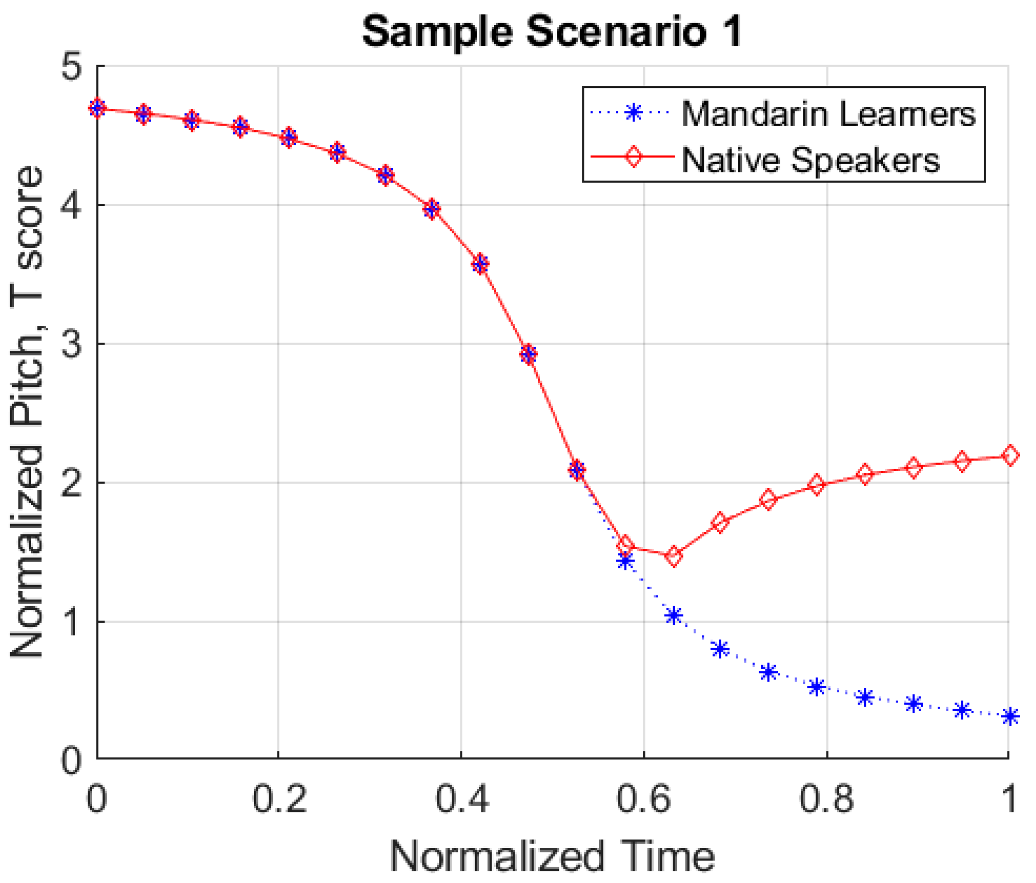
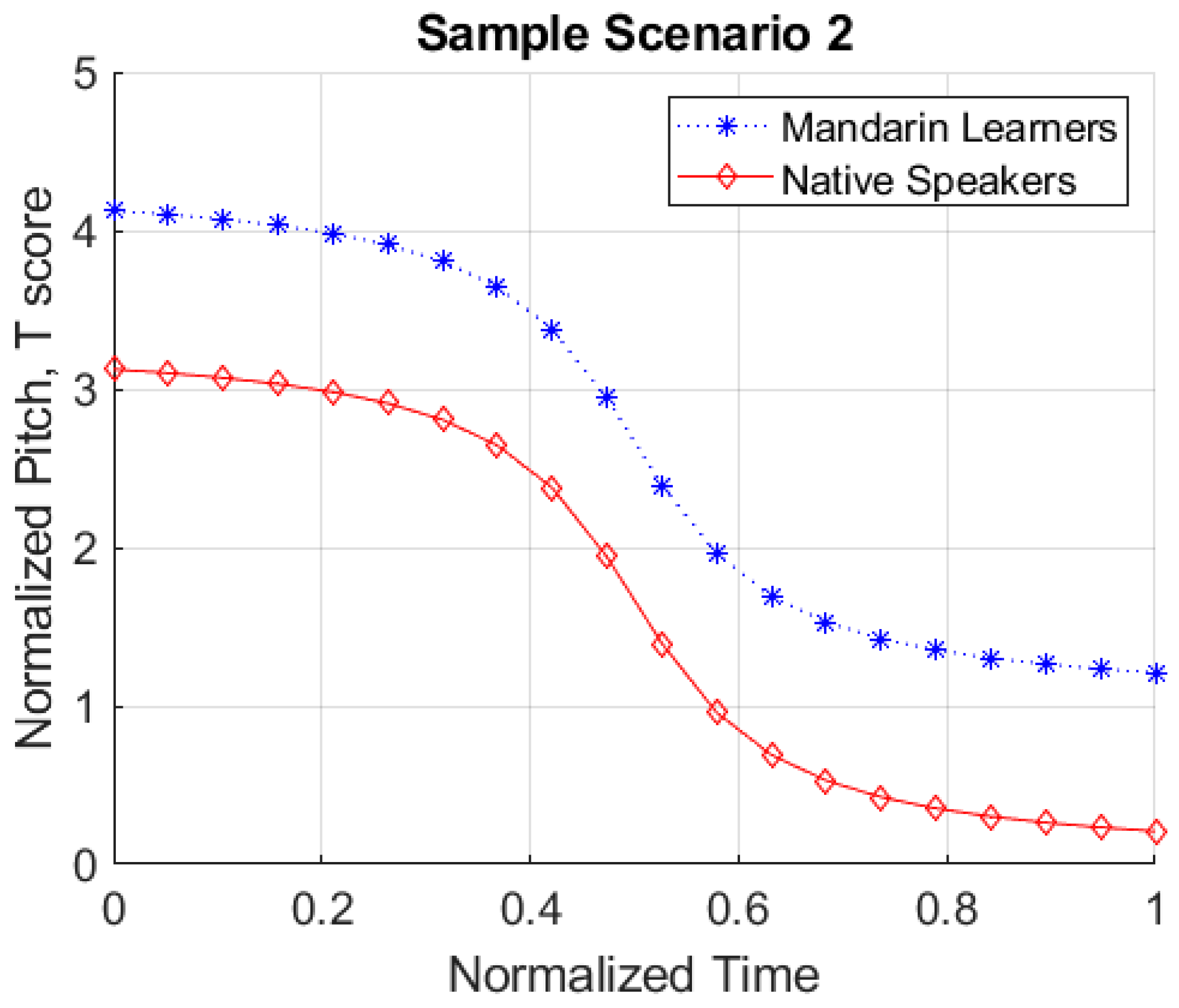
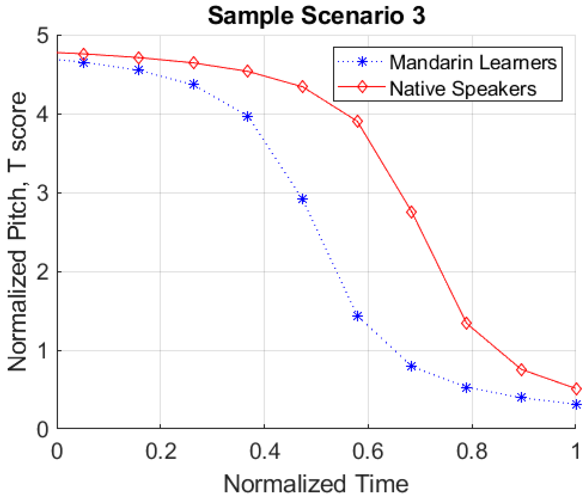
Although overall deviation scores provide a way to compare pretest and posttest productions, their calculations result in a single value, thus losing information about contour shape, height, and the temporal dimension. These aspects of tone production are crucial for comparing L1 and L2 tones. Illustrating the importance of maintaining this information, consider Figure 3, Figure 4 and Figure 5. In Figure 3, the overall shape of the L1 and L2 contours are different (i.e., matched at the beginning but not at the end). In Figure 4, while the overall shape and timing of the two contours are identical, they differ with respect to pitch height. In Figure 5, the shapes and heights are identical but differ with respect to timing (i.e., phase). It is worth noting that in each of these sample scenarios, a deviation score analysis produces identical overall deviation scores (T = 1.00).
In these scenarios, the key information about contour, height, and timing is lost when using a single overall deviation score in the analysis. Acknowledging this lack of detail, previous studies have tried to address this issue by supplementing deviation scores with qualitative analysis of time series plots (Wang et al. 2003; Zhou and Olson 2023). However, quantitative pitch height and contour analysis are necessary for statistical analyses comparing L1 and L2 tone datasets. A new type of analysis to compare tone data that includes information about these three aspects of tone (height, contour shape, timing) is necessary to capture detailed differences in tone contour comparison.

1.3. Defined Region Approach

Taking the overall deviation score as a point of departure, it is worth exploring how this calculation can be expanded to give more information about pitch height and contour. Some studies have taken a defined region approach to tone, dividing productions into specific sections or regions. For example, Liao et al. (2010) divide tones into three regions and analyze the mean F0 value for each region in their feedback system. Even though this study does not compare L1 and L2 tone productions, the defined region analysis can expand the deviation score approach.
Dividing the T value data into three regions would provide more information about where in the production the L2 tone differs from the L1 tone. Deviation scores could then be calculated for each portion of the contour, giving a quantitative measure of differences between the two datasets. This application would be useful for tone, particularly for Tone 2 and Tone 3 in Mandarin, as they vary significantly in F0 height and contour throughout their productions. This analysis would output three different scores, indicating whether the L2 productions deviated in height by producing tones higher (positive deviation score) or lower (negative deviation score) than native speaker productions.
The defined region deviation score analysis included in the current study, based on Liao et al. (2010), builds on the traditional overall deviation score calculation by providing additional information about the differences in pitch heights between productions. Yet, this analysis still fails to account for the temporal dimension, losing information about contour, and only provides an overall view of pitch height differences.

1.4. Measures for Time Series Data

To capture information about contour, height, and timing information when analyzing two sets of time series data (L1 and L2 tone), it is useful to investigate previously established algorithms for time series data outside the fields of linguistics and phonetics. Time series datasets can be found in various fields (e.g., medicine, anthropology), which has created many different algorithms for comparison (Ding et al. 2008). An integral part of comparing time series data is choosing the correct distance measure (Batista et al. 2014; Keogh et al. 2009) that captures the invariances of the specific data being explored (for a discussion of the types of invariances, see Batista et al. 2014). Invariance can be described in terms of whether or not a generalization about how variables are related is invariant or would be true if other factors changed (Woodward 2000). With respect to the current study, the distance measure would indicate the deviation between the L1 and L2 tone contours for a specific Mandarin tone. The idea of complexity invariance, which can be simply described as data that has “more peaks, valleys, and features” (Batista et al. 2014, p. 635), is a characteristic of the type of data analyzed in the current study, as tone has significant F0 movement during production, even for tones that have traditionally been described as “flat” (e.g., Tone 1 in Mandarin).
Knowing that the time series data explored in the current study is complex, the question remains about how to best measure the distance between the L1 and L2 tone time series. One particularly promising measure is known as a CID measure, proposed by Batista et al. (2014) and based on Euclidian distance (ED). ED is a popular measure to compare two-time series datasets, as it can be used to measure the similarity of two-time series datasets. Not only does ED consider the deviations between the two datasets, but it also accounts for warping effects, where two datasets exhibit the same general shape (e.g., peaks and valleys), though they are mismatched in timing. The CID measure, which adds to the traditionally-used ED measurements, provides an efficient way to compare time series data without ignoring the complex nature of these datasets, thus mitigating errors that would occur by oversimplification (Batista et al. 2014). This measure has been successfully applied to different time series datasets (for air pollutants, see Amato et al. 2020; for traffic signals and financial stock indexes, see Shang et al. 2019; for acceleration data, see Souza 2018). Without the correction factor (see Section 2.3.3) that the CID measure employs, errors and biases can be introduced from complex data being treated as simple data (Batista et al. 2014), causing data to seem more similar in terms of the measure used (i.e., ED). In terms of L1 and L2 tone, the EDs calculated for the datasets could suggest that the L2 data is closer to the L1 data than it is, leading to possible misinterpretations of how similar productions are before and after training, effectively underestimating training effects. The use of CID measures is a possible way to capture the true differences between L1 and L2 tones, without losing pertinent information about the heights, contours, and timing of productions.

1.5. The Current Study

Given the shortcomings described above with current analyses for lexical tone comparison, notably the failure of quantitative measures to account for differences in height, contour shape, and timing, this study aims to (a) explore the applicability of the CID measure proposed by Batista et al. (2014) for comparing L1 and L2 lexical tone datasets and (b) compare the applicability of this analysis to two other analyses. As such, three different analyses will be applied to existing datasets consisting of lexical tones produced by learners before (i.e., pretest) and after (i.e., posttest) a pedagogical intervention (i.e., visual feedback paradigm). The first analysis employs the calculation of single deviation score analysis, following previous studies (Wang et al. 2003; Zhou and Olson 2023). Drawing on work that has quantitatively described multiple key tonal regions (Liao et al. 2010), the second analysis consists of calculating deviation scores by region (i.e., defined region analysis). Finally, a complexity-invariant distance analysis (Batista et al. 2014) for the two-time series (L1 and L2 tone) is considered. Outcomes from these three different types of analysis will be compared.

2. Materials and Methods

2.1. Datasets

The datasets consisted of tones extracted from real disyllabic Mandarin words produced by five (four female, one male) L2 speakers (Mage = 21.2; SD = 2.0) of Mandarin (L1 = English).3 Two L1 speakers of Mandarin were also recruited to provide native speaker comparisons (Mage = 25, SD = 1).
All participants participated in a visual feedback paradigm consisting of a pretest, four interventions (one per Mandarin tone), and a posttest, completed over the course of seven weeks. Following (Offerman and Olson 2016), each intervention consisted of an initial recording, a visual comparison of the L2 lexical tone contour with a native speaker tone contour, and a re-recording in which participants attempted to produce more target-like contours. For full details of the intervention, see Zhou and Olson (2023).
The data extracted for the current study was produced during the pretest and posttest of the visual feedback study. Stimuli produced as words in isolation consisted of three repetitions of 20 real disyllabic Mandarin words with each possible tone combination represented, totaling 60 productions of the stimuli at the pretest (120 syllables) and 60 productions of these same words at the posttest (120 syllables) per speaker. All four Mandarin tones were analyzed as they are all different shapes and heights, providing a variety of productions to test the three analyses. The four syllables produced as the Neutral Tone were excluded due to their high variability (Zhang 2017). This led to 216 syllables (240–24 Neutral Tone productions) produced by each L2 speaker (108 at the pretest + 108 at the posttest). The L1 speakers also produced the target stimuli one time only, as they did not take part in the visual feedback paradigm. A sample set of stimuli can be seen below in Table 1 for Tone 1. A total of 1028 syllables were included in the final analysis (870 produced by L2 speakers + 158 produced by L1 speakers), with ~21% eliminated due to noisy data (n = 268).

2.2. Data Pre-Processing

For each target item, F0 measurements (Hz) were extracted at 10-millisecond intervals for each syllable using Praat’s (Boersma and Weenink 2022) autocorrelation algorithm with default input parameters and inputted into MATLAB v.R2023a (The MathWorks Inc. 2023). Following previous studies (Wang et al. 2003; Zhou and Olson 2023), data resampling, time normalization, and F0 normalization were performed to account for individual differences in pitch range, speech rate, and syllable context.

2.2.1. Data Resampling and Curve Fitting

To ensure the same temporal resolution (i.e., duration) for all contours, the data were resampled to have an equal number of F0 points. Contours containing more than 20 F0 points were downsampled to 20 points, while other contours with less than 20 points were only used in the analysis if they had the following: 10 or more points and points existing at the beginning and end of the production. This allowed contours with a lower but sufficient number of data points to be included in the datasets through interpolation. Some possible reasons for contours having less than 20 points are the absence of quasi-periodic structures at some points or pauses/breaks due to different speech phenomena (e.g., creaky voice). The data was interpolated using the Fourier series with seven terms, which preserves the periodic nature of tones. The formula used in MATLAB for this type of curve fitting can be seen below in Equation (1).
F 0 ~ t = a 0 + i = 1 3 a i   cos i ω t + b i sin i ω t

2.2.2. Time Normalization

To normalize time, also known as nondimensionalizing time, the following formula (Equation (2)) was used, where t corresponds to a particular point in time, and tinitial and tfinal correspond to the starting and ending points of the production, respectively.
t * = t t i n i t i a l t f i n a l t i n i t i a l

2.2.3. F0 Normalization

F 0 values were converted to their logarithms using the formula below (Equation (3)), which has been used in previous studies (e.g., Rose 1987). Fmax and Fmin correspond to the highest and lowest F 0 for a speaker, respectively, and F is a specific point of a contour. The resulting metric, referred to as the T value here on out (ranging from 0 to 5), corresponds to a 5-point pitch scale (Chao 1948).
T = 5 × log F log F m i n log F m a x l o g ( F m i n )
The ‘native norm’ (see Wang et al. 2003) was calculated to be used compared to L2 speakers’ productions. The data extracted from productions of the stimuli by the two native speakers was used to calculate this native norm, specifically by averaging the productions across each tone using the calculated T values.

2.3. Analyses

Following the calculation of the native norm, the three types of analyses explored in the current study were applied.

2.3.1. Deviation Score Analysis

The first analysis to be tested is the calculation of single overall deviation scores for each L1–L2 tone comparison based on previous studies (Wang et al. 2003; Zhou and Olson 2023). The calculation of overall deviation scores consisted of calculating the relative difference in T values between the native norm and the L2 speakers’ pretest or posttest productions at a particular point, then averaging these scores across all 20 points.

2.3.2. Defined Region Analysis

The second analysis defines different regions of normalized tone productions and then calculates deviation scores for each region, following the process described in Section 2.1. The productions were divided into three regions, beginning, middle, and end, following Liao et al. (2010), by dividing the productions into three equal nondimensionalized time regions.

2.3.3. CID Measure Analysis

The third analysis consisted of the calculation of CID measurements for each tone, comparing either pretest or posttest to the native norm. Before calculating the CID measurements, EDs for the time series datasets were calculated first. The formula to calculate ED for a two-time series can be seen below (Equation (4)). The two-time series datasets are represented by Q and C (their elements are q i and c i respectively), with a length represented by n.
E D Q ,   C = i = 1 n q i c i 2 2
The calculation of ED by itself was not sufficient for comparing time series datasets precisely due to the complexity invariance described previously. After the calculation of ED, the data remains distorted, requiring a correction factor (Batista et al. 2014). The ED between the time series is made “complexity-invariant” by adding a correction factor (CF) (Batista et al. 2014), shown below in Equation (5). CE represents a complexity estimate of a time series (Q or C).
C F Q ,   C = max ( C E Q , C E C ) m i n ( C E Q , C E C )
This was then used to solve for CID, using the formula below (Equation (6)).
C I D Q ,   C = E D ( Q ,   C ) × C F ( Q ,   C )
CID measures for each tone were then used with time series plots to visualize the distance between the L1 and L2 datasets. Two additional features were analyzed from the data used in these plots—magnitude, and phase. Magnitude corresponds to pitch height, while phase corresponds to timing. The magnitude and phase for each comparison (L2 at pretest vs. L1 or L2 at posttest vs. L1) were calculated using the process below.
The magnitude was calculated by taking the sum of the absolute value of each warping vector. This calculation gave an overall indicator of deviation of the pitch height for the comparisons (L2 pretest vs. L1 or L2 posttest vs. L1). The phase was calculated by taking the sum of the absolute value of the angle of the warping vectors with respect to the vertical axis. This calculation gave an overall indicator of deviation of the production shape (i.e., timing) for the tone comparisons.

3. Results

3.1. Deviation Score Analysis Results

The results of the deviation score calculations per Mandarin tone, or the absolute difference in T values between the native norm (L1) and L2 speakers’ T values averaged across all points in a contour (at pretest or posttest), are shown below in Table 2.
For Tone 1, the calculated deviation scores for the L2 speakers’ pretest productions (deviation score: −0.52) and posttest productions (deviation score: −0.46) suggest that the posttest productions were more L1-like than the pretest productions, as the posttest deviation score was closer to zero. Regarding Tone 2, the calculated deviation scores for the L2 speakers’ pretest productions (deviation score: 0.10) and posttest productions (deviation score: −0.05) suggest that the posttest productions were more L1-like. Tone 3 results indicate that the pretest productions (deviation score: −0.14) were more L1-like than the posttest productions (deviation score: −0.21). Tone 4 results suggest that the posttest productions (deviation score: −0.67) were more L1-like than the pretest productions (deviation score: −0.70). Taken as a whole, deviation scores are closer to zero at the posttest for Tone 1, Tone 2, and Tone 4, indicating they are more L1-like. However, these scores miss fundamental information about the pitch height and contour across productions.

3.2. Defined Region Analysis Results

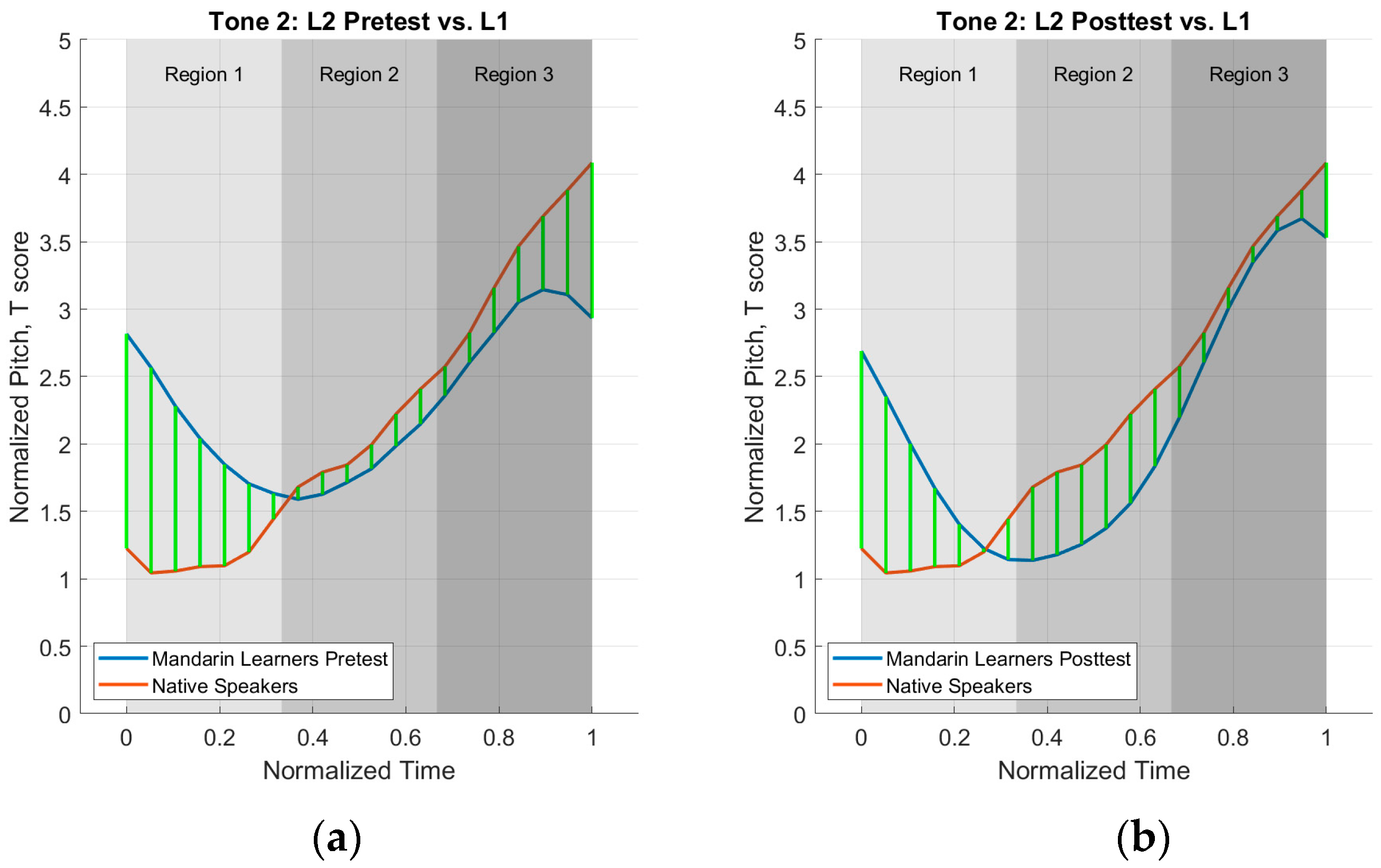
The results of the deviation score calculations for each tone per region (beginning = region 1, middle = region 2, end = region 3) can be seen below in Table 3. Visualizations of the three regions for each L1–L2 tone comparison are presented in Figure 6, Figure 7, Figure 8 and Figure 9 below. The addition of the regions in this analysis differs from the first analysis (i.e., deviation score analysis) in that it provides more information about where the L2 speakers are deviating from the L1 speakers.
Figure 6, Figure 7, Figure 8 and Figure 9, with green lines representing the matched points between two datasets (L1 and L2 tone), further illustrate differences in the datasets.
For Tone 1, the deviation scores presented in Table 3 indicate that the L2 speakers were more L1-like at the posttest in regions 2 and 3 but marginally more L1-like at the pretest in region 1. Negative scores in regions 2 and 3 at the pretest and posttest indicate a pitch height lower than the L1 speakers, while positive scores in region 1 indicate higher pitched tones. A visualization of these results can be found in Figure 6. While the first analysis showed improvement from pretest to posttest, the second defined region analysis refines this analysis by showing that improvement was limited to the middle and end of the productions.
Tone 2 results show that the L2 speakers were more L1-like at the posttest for regions 1 and 3 but more L1-like at the pretest in region 2, visualized in Figure 7. Additionally, results from Table 3 show L2 speakers’ pretest and posttest pitch heights were produced lower than the L1 speakers for regions 2 and 3 but higher than L1 speakers in region 1. This second analysis provides information on where the posttest is closer to the L1 speakers (regions 1 and 3) compared to the first analysis, which only states that the posttest deviated less from the L1 speakers than the pretest.
The results for Tone 3 presented in Table 3 show that the L2 speakers were more L1-like in regions 1 and 3 for the posttest but were more L1-like in region 2 for the pretest productions. Also, the pretest and posttest pitch heights were produced lower than the L1 speakers in regions 1 and 2 but higher than the L1 speakers in region 3 (Figure 8). Like Tone 1 and Tone 2 results, Tone 3 results are more nuanced than the single overall deviation score calculation.
Tone 4 results in Table 3 show that L2 speakers were marginally more L1-like at the posttest in region 2 but more L1-like at the pretest for regions 1 and 3. Pretest and posttest pitch heights were produced lower than L1 speakers for regions 1 and 2 and higher than L1 speakers for region 3, as shown in Figure 9. With the addition of the deviation scores for the three regions, more information is provided on where the L2 tone is more L1-like at the pretest (regions 1 and 3) compared to the first analysis.

3.3. CID Measure Analysis Results

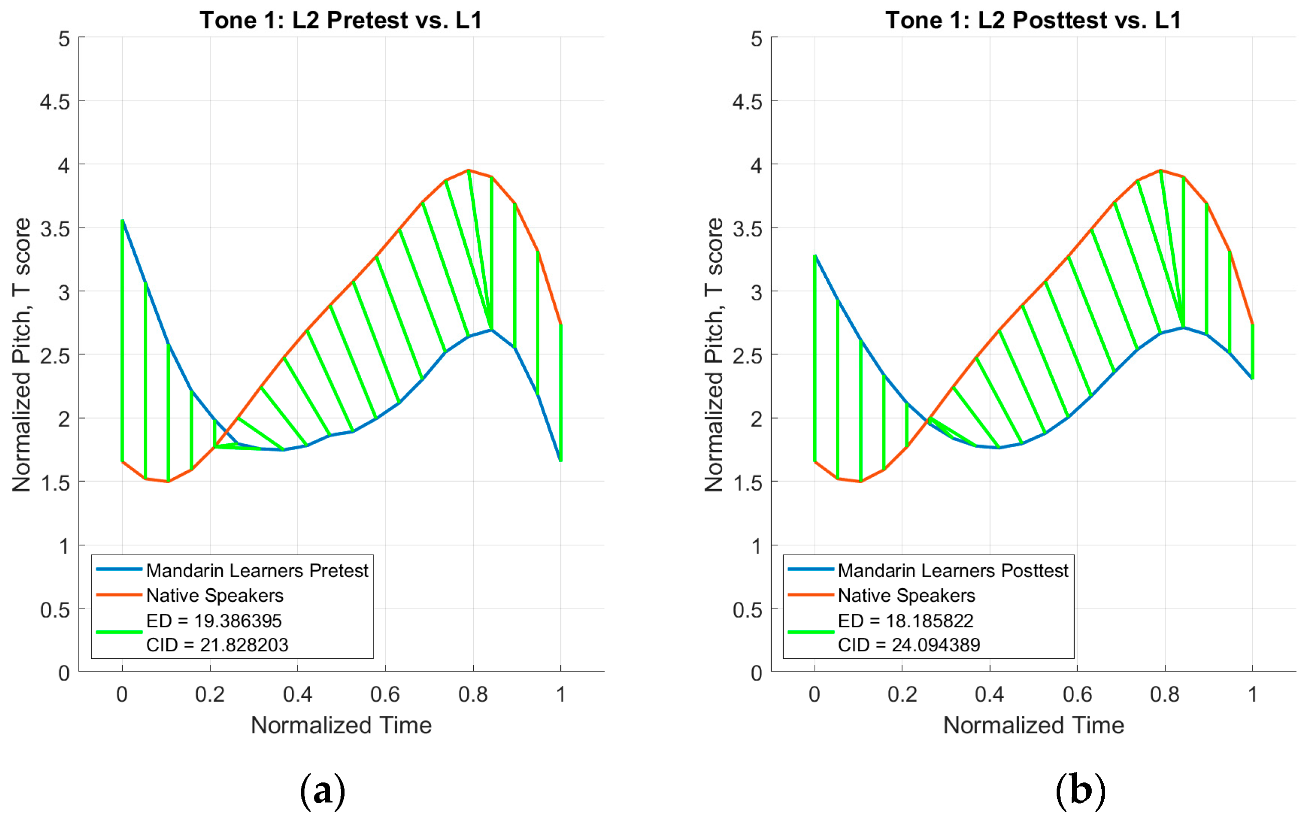
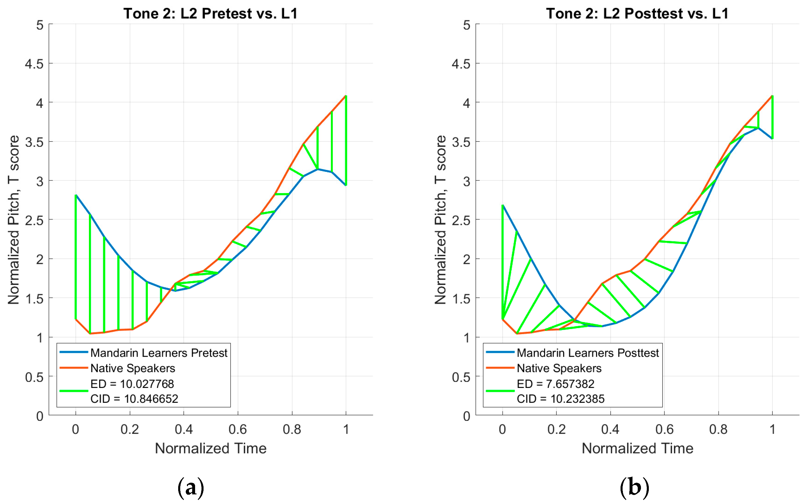
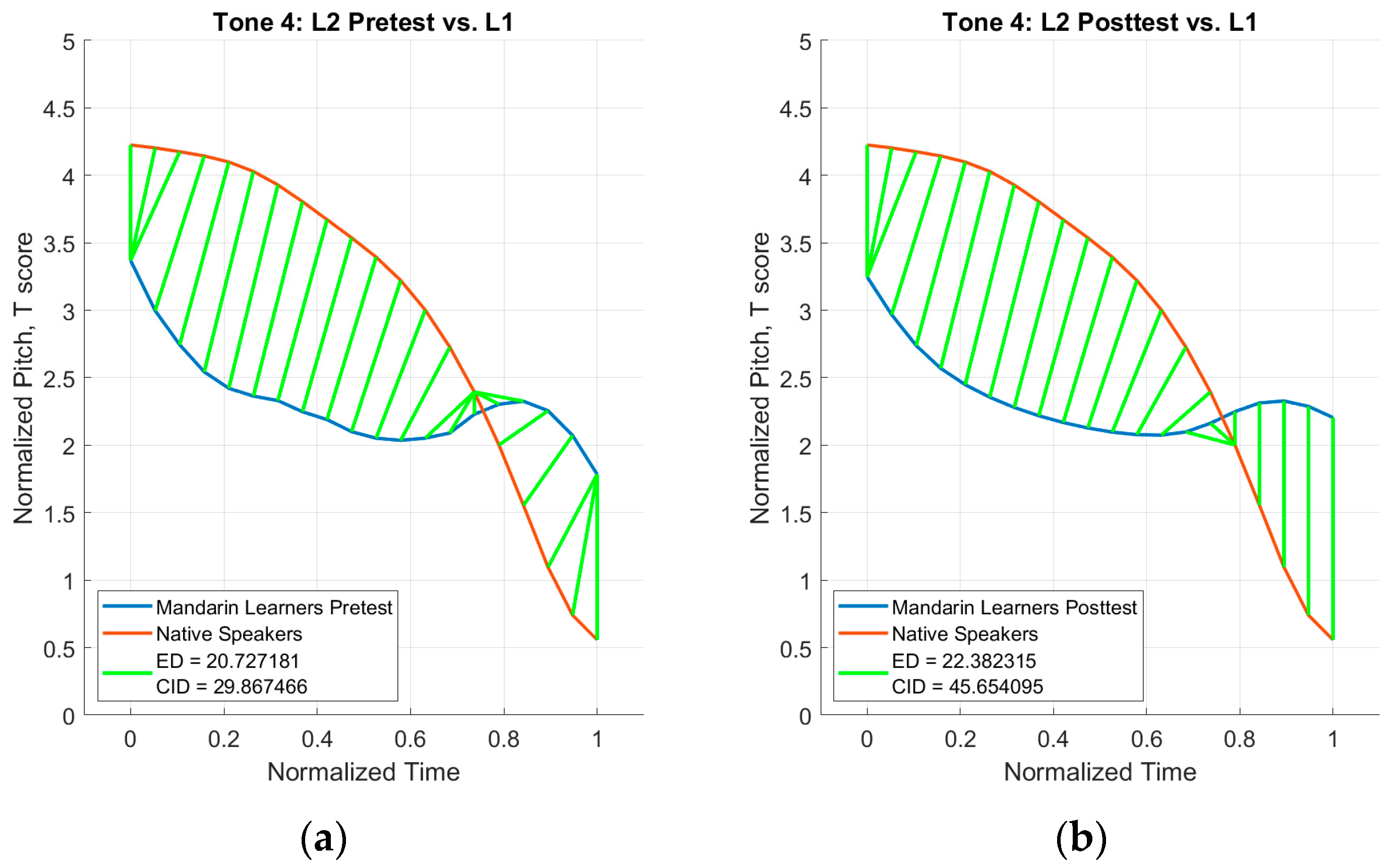
Results from the application of the CID measure to the two-time series are shown below in Figure 10, Figure 11, Figure 12 and Figure 13 for the pretest and posttest productions. Both the ED and CID measure (corrected ED) are presented in the legends of the time series plots. Green lines correspond to the distance between L1 and L2 T values at a given point matched for magnitude and phase. Information on magnitude and phase are also presented for each tone in Table 4, with scores closer to zero indicating more L1-like production.
For Tone 1, the calculated CID measures shown in Figure 10 for the pretest (21.83) and posttest (24.09) productions indicate that the L2 speakers’ pretest productions were closer in distance to the L1 speakers’ productions. Notably, the original ED calculations for Tone 1 resulted in the posttest (ED: 18.19) productions being closer to the L1 productions than the pretest (ED: 19.39) productions. The calculated magnitudes for Tone 1 shown in Table 4 indicate that the pitch height was more L1-like at the posttest (7.69) than at the pretest (8.58). However, the phases suggest that the timing was more L1-like at the pretest (48.84) than at the posttest (78.63). The results from the CID measure analysis provide additional information when compared to the first two analyses, specifically a more accurate measurement of distance that shows pretest productions deviated less than posttest productions, which was the opposite of the findings from the first two analyses. This third analysis also provided information about which aspect the L2 tone deviated in more at the posttest, namely phase (timing).
The CID measures for Tone 2 shown in Figure 11 indicate that the L2 speakers’ posttest productions (CID measure: 10.23) were closer in distance to the L1 speakers than the pretest productions (CID measure: 10.85). The calculated magnitudes and phases for Tone 2 shown in Table 4 indicate that the pitch height and timing were more L1-like at the posttest (magnitude: 2.82, phase: 96.68) than at the pretest (magnitude: 3.63, phase: 113.04). This provides more information when compared to the first two analyses, specifically that the timing and pitch height were more L1-like at the posttest.
For Tone 3, the CID measures shown in Figure 12 indicate that the L2 speakers’ pretest productions (CID measure: 23.82) were closer in distance to the L1 speakers than the posttest productions (CID measure: 26.77). Regarding the magnitude (pitch height) for Tone 3 shown in Table 4, the pretest productions (17.65) were marginally more L1-like than the posttest productions (17.94). However, for phases, the Tone 3 posttest productions (43.17) were more L1-like than the pretest productions (44.00). Similar to Tone 1 and Tone 2 results, the third analysis shows a more detailed analysis, specifically showing that the lack of improvement at the posttest was due to magnitude, not phase, even though the changes were marginal.
The CID measures for Tone 4 shown in Figure 13 indicate that the L2 speakers’ pretest productions (CID measure: 29.87) were closer in distance to the L1 speakers than the posttest productions (CID measure: 45.65). Results for Tone 4 in Table 4 show that the magnitude was more L1-like at the pretest (18.37) than the posttest (19.91), while the phase was more L1-like at the posttest (46.66) than at the pretest (62.99).
The CID measure analysis results indicate an improvement in the distance between the L1 and L2 productions at the posttest for Tone 2 only. In magnitude (pitch height), calculated magnitudes were closer to zero (more L1-like) at the posttest for Tone 1 and Tone 2 but closer to zero at the pretest for Tone 3 and Tone 4. Regarding phase (timing), phases were closer to zero at the posttest for Tone 2, Tone 3, and Tone 4 but closer to zero at the pretest for Tone 1. The CID measure analysis suggests that L2 learners improved with respect to timing, with mixed results for pitch height. The CID measure analysis gives information about the general distance between the productions, magnitude, and phase information.

4. Discussion

The current study investigated (a) the applicability of the CID measure proposed by Batista et al. (2014) to L1 and L2 tone datasets and (b) the comparison of three types of analyses for comparing L1 and L2 tone.

4.1. Exploration of the Analyses

The deviation score analysis gave a single score for each comparison. From these overall deviation scores, one can analyze how close or far L2 speakers’ pretest or posttest productions are from the L1 speakers’ productions or how close the pretest and posttest productions are to each other. Applying these results to the testing of the visual feedback paradigm, the results can show which tones were produced in a more L1-like way (Tone 1, Tone 2, and Tone 4 in the current example study). However, averaging the T scores across time for a given tone erases the temporal dimension of the productions, failing to provide any information about pitch height or contour. This previously used method (e.g., Wang et al. 2003) is insufficient for describing differences between L1 and L2 tone, particularly in specifying where and in which aspects L2 productions deviate from L1 productions.
The second analysis, performed by calculating deviation scores for three regions of the productions, resulted in three scores for each comparison. This analysis gives information on which regions L2 speakers are L1-like and in which direction the pitch height differs (positive value = higher pitch than L1 speakers, negative value = lower pitch than L1 speakers). The results of the defined region analysis suggest that the change from pretest to posttest differed by region. Specifically, participants showed improvement in regions 2 and 3 for some tones (Tone 1 and 4), and improvement in regions 1 and 3 for other tones (Tone 2 and 3), showing that L2 speakers became more L1-like in their productions (Tone 1, Tone 2, and Tone 3), with improvement being found in the aforementioned regions. Although the results of this analysis give more information than the first analysis, information about pitch height and contour is still lost from the loss of the temporal dimension. The deviation scores calculated for each region can only provide information about whether the pretest or posttest was closer to the L1 data in specific areas but does not provide detailed information about contour.
The third analysis tested, performed through the calculation of CID measures, provides critical information about the timing of the productions. While the overall CID analysis showed improvement for Tone 2 only, a more nuanced analysis of magnitude (height) and phase (timing) suggests that magnitude improved for Tones 1 and 2 while timing improved for Tones 2, 3, and 4. Without the correction factor introduced in the CID measure calculation, the ED calculated for one of the tones (Tone 1) would have indicated the opposite results (posttest being more L1-like instead of pretest being more L1-like). The lack of this correction factor in the first two analyses can yield incorrect assumptions about the improvement (or lack of improvement) for Tone 1 from pretest to posttest, as the overall deviation score showed more L1-like productions at the posttest, with the deviation scores by region supporting this (more L1-like at posttest for two regions). This may provide evidence for the strength of the CID measure analysis, as this more robust analysis provides a more detailed and accurate measurement, leading to a more accurate depiction of the learners’ improvement. Additionally, the calculation of magnitude and phase is critical to this analysis as it provides information about pitch height and timing, providing more information on how native-like learners were in their productions, which was lost in the first two analyses.

4.2. Conclusions from the Current Study

As more research focuses on the development of methods for teaching L2 suprasegmental features, which are important for comprehensibility and intelligibility (Munro and Derwing 1995), there is a growing need for quantitative methods to analyze and compare tone contours. This paper details three approaches (deviation scores, defined region analysis, and CID measure analysis). While the overall number of participants in the current study is limited, these participants produced many tokens, which served as a test case for the novel CID measure analysis. Future research may seek to compare these analyses across larger numbers of participants, further highlighting the differences in analyses. Returning to the first objective of the paper (i.e., exploring three different types of analyses), although these calculations are fundamentally different, it is important to note the difference between the conclusions that can be drawn from the first analysis and the third analysis, specifically that the deviation scores indicate the L2 speakers’ posttest scores being more L1-like for a different set of tones (Tone 1, Tone 2, Tone 4) than the CID measures indicate in terms of distance (Tone 2 only). As the CID measure calculation considers the complexity invariance of the data (i.e., through the introduction of a correction factor discussed above), it is more robust than the calculation of deviation scores, which disregards the temporal dimension and the complex nature of the data. Results from the CID measure analysis show a more mathematically powerful depiction of the level of tone improvement, while the first two analyses show a less accurate depiction of tone improvement, leading to differing results between the three types of analyses.
Returning to the study’s second objective, whether this measure could be applied to the comparison of L1 and L2 tone datasets, results show that the CID measure analysis can be applied and provide a measure of difference that is mathematically more powerful than previous analyses. Results from this study suggest that the analysis using the CID measure provides a more nuanced analysis of the differences between L1 and L2 tone datasets. Specifically, along with the valuable information gained from the CID measurements themselves, the output of the analysis also provided information on magnitude (i.e., pitch height) and phase (i.e., timing). This information on timing can provide learners with an understanding of how ‘on-time’ they were with the native speakers’ productions.
From a methodological perspective, the paper has demonstrated that the CID measure provides significant benefits over the other two analyses. For research analyses that seek to document or assess the development of L2 lexical tone over time, either resulting from instruction or naturalistic acquisition, the CID measure significantly improves over prior quantitative methodologies. Accounting for the role of phase in contour production, rather than assuming that F0 data are necessarily matched at a given normalized timepoint, provides a more faithful representation of the differences between the two contours. Traditional methods, such as the deviation score analysis may lead to incorrect assumptions about the tone improvement after the intervention, as evidenced by this analysis showing improvement in more tones than the CID measure analysis. Moreover, while outside the scope of the current paper, this method lends itself to statistical analyses that account for phase more so than the traditional qualitative analyses.
From a pedagogical perspective, the utility of the visualizations and quantitative measures presented here should be carefully considered. With respect to the visualization of L2 lexical tone, Olson (2014) argues that visual feedback may rely on the inherent ‘intuitiveness’ of a visual representation. Applying the concept of intuitive interpretation to the methods used here, it is possible that the matched time series plots, with lines indicating the overall shift in phase (e.g., Figure 6), may provide better information for learners about the overall timing of their tone contours. Concerning the quantitative measures presented here, there appears to be a clear trade-off between interpretability (by learners) and complexity. While the deviation score provides a fairly easy-to-understand measure (closer to zero = more native-like), it lacks significant detail about how the two contours differ. In contrast, the CID measure provides detailed information about distance, height, and timing but may be hard for learners to interpret. While future research should study this question in more depth, it is possible that the main benefit to learners comes from the visualization, rather than quantitative measurement, of L2 contours. Future research should also explore applying this novel analysis to types of training paradigms other than visual feedback. The third analysis may provide pedagogical benefits for other methods of tone training that do not rely on visualizations alone.

Author Contributions

Conceptualization, A.Z. and D.J.O.; methodology, A.Z. and D.J.O.; software, A.Z.; validation, A.Z. and D.J.O.; formal analysis, A.Z.; investigation, A.Z.; resources, A.Z. and D.J.O.; data curation, A.Z.; writing—original draft preparation, A.Z. and D.J.O.; writing—review and editing, A.Z. and D.J.O.; visualization, A.Z. and D.J.O.; supervision, D.J.O.; project administration, D.J.O.; funding acquisition, A.Z. and D.J.O. All authors have read and agreed to the published version of the manuscript.

Funding

This research received no external funding.

Institutional Review Board Statement

The study was conducted in accordance with the Declaration of Helsinki and approved by the Institutional Review Board of Purdue University (IRB-2021-1512 approved on 11-09-2021)” for studies involving humans.

Informed Consent Statement

Informed consent was obtained from all participants involved in the study.

Data Availability Statement

The data presented in this study are available on request from the corresponding author. The data are not publicly available to keep participants’ audio files confidential.

Conflicts of Interest

The authors declare no conflict of interest.

Notes

1
Also, it is worth noting emerging research on L2 tone evaluations via machine learning. This research has mainly focused on the development of networks or models for identifying mispronounced L2 tone (e.g., Cheng 2012; Li et al. 2019).
2
Although both prior analyses and those examined in the current paper use native speaker productions as a benchmark for L2 comparisons, it should be noted intelligibility and comprehensibility (for a discussion, see Munro and Derwing 1995) rather than native-like production should be the aim for most L2 learners.
3
Data from four speakers was previously presented in Zhou and Olson (2023).

References

  1. Amato, Federico, Mohamed Laib, Fabian Guignard, and Mikhail Kanevski. 2020. Analysis of air pollution time series using complexity-invariant distance and information measures. Physica A: Statistical Mechanics and Its Applications 547: 1–9. [Google Scholar] [CrossRef]
  2. Batista, Gustavo E. A. P. A., Eamonn Keogh, Oben M. Tataw, and Vinicius M. A. de Souza. 2014. CID: An efficient complexity-invariant distance for time series. Data Mining and Knowledge Discovery 28: 634–69. [Google Scholar] [CrossRef]
  3. Boersma, Paul, and David Weenink. 2022. Praat–Doing Phonetics by Computer (Version 6.2.23). [Computer Program]. Available online: www.praat.org (accessed on 15 May 2023).
  4. Chao, Yuen R. 1948. Mandarin Primer. Cambridge: Harvard University Press. [Google Scholar]
  5. Chen, Gwang-tsai. 1974. The pitch range of English and Chinese speakers. Journal of Chinese Linguistics 2: 159–71. [Google Scholar]
  6. Chen, Mengtian. 2022. Computer-aided feedback on the pronunciation of Mandarin Chinese tones: Using Praat to promote multimedia foreign language learning. Computer Assisted Language Learning 35: 1–26. [Google Scholar] [CrossRef]
  7. Cheng, Jian. 2012. Automatic tone assessment of non-native Mandarin speakers. Paper presented at 13th Annual Conference of the International Speech Communication Association, Portland, OR, USA, September 9–13; Baixas: International Speech Communication Association (ISCA), pp. 1299–302. [Google Scholar] [CrossRef]
  8. Chun, Dorothy M. 1989. Teaching tone and intonation with microcomputers. CALICO Journal 7: 21–46. [Google Scholar] [CrossRef]
  9. Chun, Dorothy M., Yan Jiang, Justine Meyr, and Rong Yang. 2015. Acquisition of L2 Mandarin Chinese tones with learner-created tone visualizations. Journal of Second Language Pronunciation 1: 86–114. [Google Scholar] [CrossRef]
  10. Ding, Hui, Goce Trajcevski, Peter Scheuermann, Wang Xiaoyue, and Eamonn Keogh. 2008. Querying and mining of time series data: Experimental comparison of representations and distance measures. Proceedings of the VLDB Endowment 1: 1542–52. [Google Scholar] [CrossRef]
  11. Esling, Philippe, and Carlos Agon. 2012. Time-series data mining. ACM Computing Surveys 45: 1–34. [Google Scholar] [CrossRef]
  12. He, Yunjuan, Qian Wang, and Ratree Wayland. 2016. Effects of different teaching methods on the production of Mandarin tone 3 by English-speaking learners. Chinese as a Second Language 51: 252–65. [Google Scholar] [CrossRef]
  13. Keogh, Eamonn, Li Wei, Xiaopeng Xi, Michail Vlachos, Sang-Hee Lee, and Pavlos Protopapas. 2009. Supporting exact indexing of arbitrarily rotated shapes and periodic time series under Euclidean and warping distance measures. The VLDB Journal 18: 611–30. [Google Scholar] [CrossRef]
  14. Li, Man, and Robert DeKeyser. 2017. Perception practice, production practice, and musical ability in L2 Mandarin tone-word learning. Studies in Second Language Acquisition 39: 593–620. [Google Scholar] [CrossRef]
  15. Li, Wei, Nancy F. Chen, Sabato M. Siniscalchi, and Chin-Hui Lee. 2019. Improving mispronunciation detection of Mandarin tones for non-native learners with soft-target tone labels and BLSTM-based deep tone models. IEEE/ACM Transactions on Audio, Speech, and Language Processing 27: 2012–24. [Google Scholar] [CrossRef]
  16. Liao, Hsien-Cheng, Jiang-Chun Chen, Sen-Chia Chang, Ying-Hua Guan, and Chin-Hui Lee. 2010. Decision tree-based tone modeling with corrective feedback for automatic Mandarin tone assessment. Paper presented at 11th Annual Conference of the International Speech Communication Association, Chiba, Japan, September 26–30; Baixas: International Speech Communication Association (ISCA), pp. 602–5. [Google Scholar] [CrossRef]
  17. Munro, Murray J., and Tracey M. Derwing. 1995. Foreign accent, comprehensibility, and intelligibility in the speech of second language learners. Language Learning 45: 73–97. [Google Scholar] [CrossRef]
  18. Offerman, Heather M., and Daniel J. Olson. 2016. Visual feedback and second language segmental production: The generalizability of pronunciation gains. System 59: 45–60. [Google Scholar] [CrossRef]
  19. Olson, Daniel J. 2014. Benefits of visual feedback on segmental production in the L2 classroom. Language Learning & Technology 18: 173–92. Available online: https://llt.msu.edu/issues/october2014/olson.pdf (accessed on 23 May 2023).
  20. Olson, Daniel J., and Heather M. Offerman. 2021. Maximizing the effect of visual feedback for pronunciation instruction: A comparative analysis of three approaches. Journal of Second Language Pronunciation 7: 89–115. [Google Scholar] [CrossRef]
  21. Rose, Phil. 1987. Considerations in the normalization of the fundamental frequency of linguistic tone. Speech Communication 6: 343–51. [Google Scholar] [CrossRef]
  22. Schmidt, Richard. 1995. Consciousness and foreign language learning: A tutorial on the role of attention and awareness in learning. In Attention and Awareness in Foreign Language Learning. Edited by Richard Schmidt. Honolulu: University of Hawai’i Press, pp. 1–63. [Google Scholar]
  23. Shang, Du, Pengjian Shang, and Liu Liu. 2019. Multidimensional scaling method for complex time series feature classification based on generalized complexity-invariant distance. Nonlinear Dynamics 95: 2875–92. [Google Scholar] [CrossRef]
  24. Shen, Xiaonan S. 1989. Toward a register approach in teaching Mandarin tones. Journal of the Chinese Language Teachers Association 24: 27–47. [Google Scholar]
  25. Singh, Leher, and Charlene S. L. Fu. 2016. A new view of language development: The acquisition of lexical tone. Child Development 87: 834–54. [Google Scholar] [CrossRef]
  26. Souza, Vinicius M. A. 2018. Asphalt pavement classification using smartphone accelerometer and complexity invariant distance. Engineering Applications of Artificial Intelligence 74: 198–211. [Google Scholar] [CrossRef]
  27. The MathWorks Inc. 2023. Matlab Version 9.14.0 (R2023a). [Computer Program]. Available online: www.mathworks.com (accessed on 23 May 2023).
  28. Wang, Xinchun. 2012. Auditory and visual training on Mandarin tones: A pilot study on phrases and sentences. International Journal of Computer-Assisted Language Learning and Teaching 2: 16–29. [Google Scholar] [CrossRef]
  29. Wang, Yue, Allard Jongman, and Joan A. Sereno. 2003. Acoustic and perceptual evaluation of Mandarin tone productions before and after perceptual training. The Journal of the Acoustical Society of America 113: 1033–43. [Google Scholar] [CrossRef] [PubMed]
  30. Wiener, Seth, Marjorie K. M. Chan, and Kiwako Ito. 2020. Do explicit instruction and high variability phonetic training improve nonnative speakers’ Mandarin tone productions? The Modern Language Journal 104: 152–68. [Google Scholar] [CrossRef]
  31. Woodward, James. 2000. Explanation and invariance in the special sciences. The British Journal for the Philosophy of Science 51: 197–254. Available online: https://www.jstor.org/stable/3541803 (accessed on 1 April 2023). [CrossRef]
  32. Yang, Chunsheng, and Marjorie K. M. Chan. 2010. The perception of Mandarin Chinese tones and intonation by American learners. Journal of the Chinese Language Teachers Association 45: 7–36. [Google Scholar]
  33. Yip, Moira. 2002. Tone. Cambridge: Cambridge University Press. [Google Scholar]
  34. Zhang, Hang. 2017. The effect of theoretical assumptions on pedagogical methods: A case study of second language Chinese tones. International Journal of Applied Linguistics 27: 363–82. [Google Scholar] [CrossRef]
  35. Zheng, Annie, Yukari Hirata, and Spencer D. Kelly. 2018. Exploring the effects of imitating hand gestures and head nods on L1 and L2 Mandarin tone production. Journal of Speech, Language, and Hearing Research 61: 2179–95. [Google Scholar] [CrossRef]
  36. Zhou, Alexis, and Daniel Olson. 2023. The use of visual feedback to train L2 lexical tone: Evidence from Mandarin phonetic acquisition. In Proceedings of the 13th Pronunciation in Second Language Learning and Teaching Conference. Edited by R. I. Thomson, T. M. Derwing, J. M. Levis and K. Hiebert. St. Catharines: Brock University. [Google Scholar] [CrossRef]
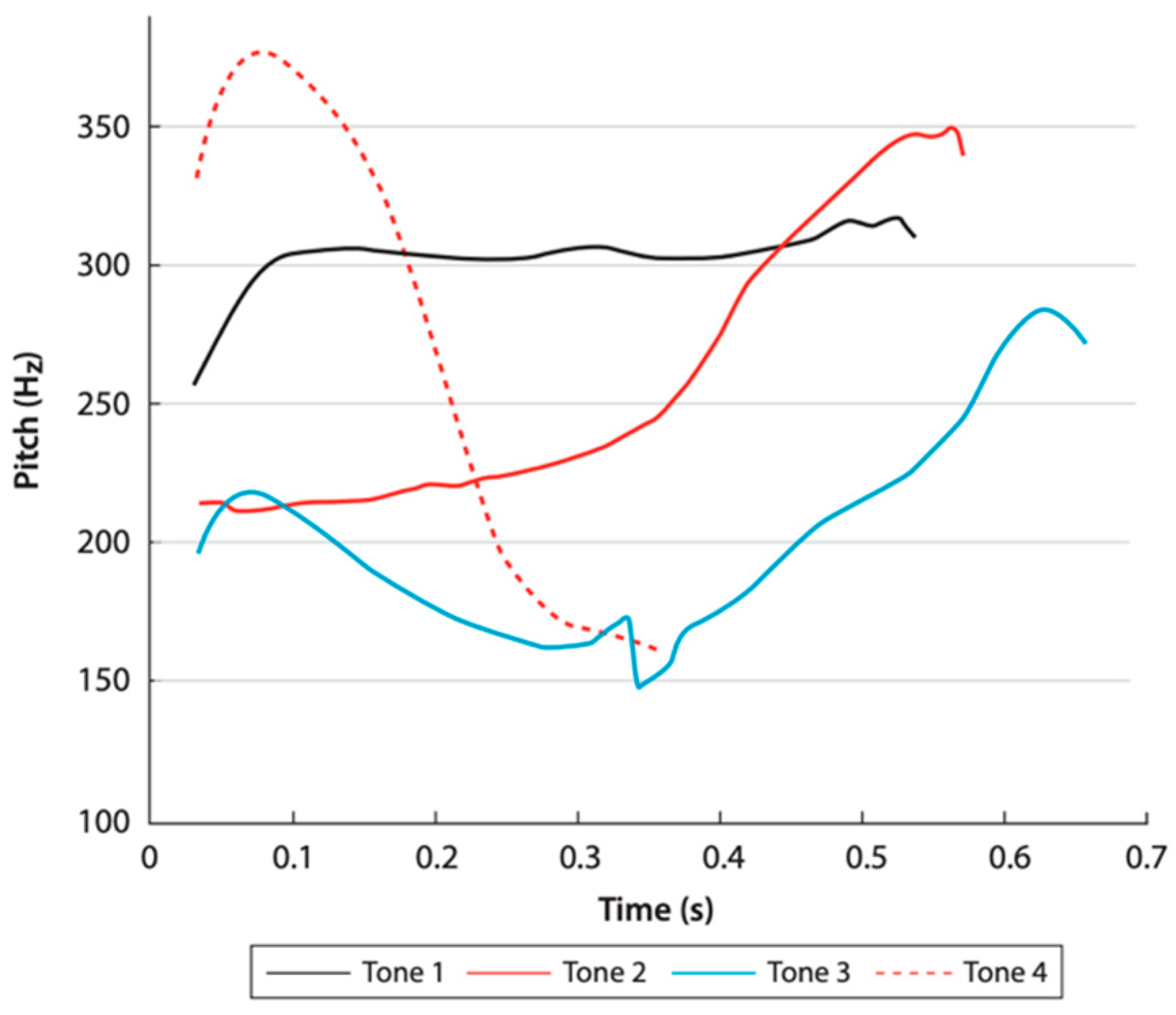
Figure 1. Acoustic visualization of the Mandarin tones. From Chun et al. (2015, p. 87). © John Benjamins. Reprinted with permission.
Languages 08 00209 g001
Figure 2. L1 vs. L2 pretest and posttest for Mandarin Tone 1. From Zhou and Olson (2023, p. 10).
Languages 08 00209 g002
Figure 3. Sample scenario 1.
Languages 08 00209 g003
Figure 4. Sample scenario 2.
Languages 08 00209 g004
Figure 5. Sample scenario 3.
Languages 08 00209 g005
Figure 6. Tone 1 deviation plots. (a) L1 vs. L2 pretest averages; (b) L1 vs. L2 posttest averages.
Languages 08 00209 g006
Figure 7. Tone 2 deviation plots. (a) L1 vs. L2 pretest averages; (b) L1 vs. L2 posttest averages.
Languages 08 00209 g007
Figure 8. Tone 3 deviation plots. (a) L1 vs. L2 pretest averages; (b) L1 vs. L2 posttest averages.
Languages 08 00209 g008
Figure 9. Tone 4 deviation plots. (a) L1 vs. L2 pretest averages; (b) L1 vs. L2 posttest averages.
Languages 08 00209 g009
Figure 10. Tone 1 distance plots. (a) L1 vs. L2 pretest averages; (b) L1 vs. L2 posttest averages.
Languages 08 00209 g010
Figure 11. Tone 2 distance plots. (a) L1 vs. L2 pretest averages; (b) L1 vs. L2 posttest averages.
Languages 08 00209 g011
Figure 12. Tone 3 distance plots. (a) L1 vs. L2 pretest averages; (b) L1 vs. L2 posttest averages.
Languages 08 00209 g012
Figure 13. Tone 4 distance plots. (a) L1 vs. L2 pretest averages; (b) L1 vs. L2 posttest averages.
Languages 08 00209 g013
Table 1. Sample stimuli for Tone 1.
Tone CombinationChinese CharactersPinyinTranslation
T1-T0心思xīnsithoughts
T1-T1开工kāigōnggo into operation
T1-T2天文tiānwénastronomy
T1-T3经理jīnglǐmanager
T1-T4医院yīyuànhospital
Table 2. Pretest and posttest mean deviation scores per tone.
PretestPosttest
Tone 1−0.52−0.46
Tone 20.10−0.05
Tone 3−0.14−0.21
Tone 4−0.70−0.67
Table 3. Pretest and posttest mean deviation scores per region.
Region 1Region 2Region 3
PretestPosttestPretestPosttestPretestPosttest
Tone 10.670.69−1.05−1.03−1.23−1.06
Tone 20.960.62−0.14−0.54−0.52−0.25
Tone 3−1.24−1.19−0.60−0.801.421.37
Tone 4−1.43−1.46−1.27−1.270.570.65
Table 4. Magnitude and phase calculations for pretest and posttest per tone.
MagnitudePhase
PretestPosttestPretestPosttest
Tone 18.587.6948.8478.63
Tone 23.632.82113.0496.68
Tone 317.6517.9444.0043.17
Tone 418.3719.9162.9946.66
Disclaimer/Publisher’s Note: The statements, opinions and data contained in all publications are solely those of the individual author(s) and contributor(s) and not of MDPI and/or the editor(s). MDPI and/or the editor(s) disclaim responsibility for any injury to people or property resulting from any ideas, methods, instructions or products referred to in the content.