A Practical Interlacing-Based Coverage Path Planning Method for Fixed-Wing UAV Photogrammetry in Convex Polygon Regions

Abstract

This paper investigates the coverage path planning problem for a fixed-wing UAV in convex polygon regions with several practical task requirements in photogrammetry considered. A typical camera model pointing forward-down for photogrammetric application is developed. In addition, the coordinates of the region vertices are converted from the WGS-84 coordinate system to the local ENU coordinate system for path planning convenience. The relationship between the minimum turning radius and the camera footprint is fully studied and the span coefficient of the fixed-wing UAV is first proposed. A novel flight pattern, named as the interlaced back-and-forth pattern in this paper, is presented accordingly. The proposed algorithm is compared with a traditional back-and-forth pattern in mathematics and several important results are given. Then, a practical low-computation algorithm for waypoints generation is developed. Finally, simulation results validate the effectiveness of the proposed method.

1. Introduction

For the past few years, unmanned aerial vehicles (UAVs) have been widely used in precision agriculture [1], terrain mapping [2], battlefield surveillance [3], search and rescue [4], and disaster management [5], etc. When performing these applications, the UAVs acquire high-resolution images that can be elaborated with PaRS techniques to obtain metric products (for example DEM, orthomosaics, etc.) [6]. In photogrammetry, a large number of overlapping aerial images taken orthogonal to the ground need to be stitched together using structure from motion (SFM) algorithms to generate what is known as an “orthophoto” [7]. Lots of commercially available photogrammetry software packages can be used to produce a digital elevation model (DEM) of the region of interest (ROI), which can then be used to extract valuable information on the surveyed areas [8].

The task of generating a path that covers the entire ROI, considering the vehicle’s motion restrictions and sensor characteristics, is called coverage path planning (CPP) [9]. UAV coverage path planning can usually be carried out by either a rotary-wing or fixed-wing UAV. When performing photogrammetric applications, the UAV is equipped with a camera, fixed directly to the airframe or mounted on a gimbal, pointing straight down or forward-down [10,11]. Rotary-wing UAVs, such as quadcopters and hexacopters, are capable of performing vertical take-off and landing (VTOL), low-altitude flights, and hovering tasks. However, these platforms have limited payload and endurance. The typical flight time for a rotary-wing UAV is less than half an hour, meaning only a small region can be imaged [12]. As for fixed-wing UAVs, they are less maneuverable than rotor drones and are not able to perform hovering tasks, but they can carry heavier payloads and have much higher endurance in comparison with rotary-wing vehicles. A single flight of a fixed-wing UAV normally lasts more than an hour [13]. Therefore, fixed-wing UAVs are more ideal for photogrammetry in a large detection area, which is the focus of this paper.

When dealing with a CPP problem, there are two questions that immediately come to mind: how to process the region of interest to simplify the path planning problem while guaranteeing complete coverage, and how to design an appropriate flight pattern in view of the practical situation. For the former, region decomposition has been studied in much of the literature and achieved fruitful results. No decomposition [14], exact cellular decomposition [15], and approximate cellular decomposition [16] are three main categories of decomposition methods developed in the literature. There is no need for decomposition in regular-shaped and non-complex areas of interest, such as rectangular areas. The exact cellular decomposition method decomposes the workspace into sub-regions, also called cells, whose re-union exactly occupy the ROI. This method is usually applied to an irregular region [17], a concave region [18], and a region with obstacles [19], and these types of regions are mostly decomposed in convex sub-regions in order to reduce the concavities and simplify coverage by boustrophedon decomposition [20], and so on. As for approximate cellular decomposition, it discretizes the region of interest with an irregular shape into a set of regular cells in the form of squares [21], hexagons [22], or triangles. Then, grid-based methods such as the wavefront algorithm [23] and the spanning tree coverage (STC) algorithm [24] are applied over approximate areas to generate coverage paths. However, the path generated tends to be erratic and contains many sharp turns which violate the dynamic constraints of fixed-wing UAVs. Hence the grid-based methods are more commonly utilized with rotary-wing UAVs. Coming back to fixed-wing UAVs, it is not difficult to conclude that a fundamental and practical problem for the UAV is path planning in a convex polygon region, which will be studied in this paper.

In addition, it is worth paying attention in coverage path planning to the flight patterns of UAVs. Two simple geometric flight patterns that are employed most commonly in real-world scenarios are back-and-forth (BF) and spiral (SP), especially for fixed-wing UAVs with maneuver constraints. For a spiral flight pattern, the flight path is straight lines with 90 degrees turns, starting from the center of the ROI, and expanding outward or vice versa [25]. The back-and-forth pattern is also known as boustrophedon or zigzag movement; in this type of movement, the UAV executes long straight flights and 180-degree turning maneuvers when reaching the boundaries [26]. These scan-type paths (a group of parallel lines covering a certain area) are naturally suitable for UAV photogrammetry applications. As a result, there is no doubt that the BF pattern is widely utilized in photogrammetry with fixed-wing UAVs.

Finally, when it comes to the performance metrics of complete coverage path planning, the total traveled distance or the path length [27], coverage flight time [28], energy consumption [29], and the number of turns [30] are most commonly found in the literature. Among them, the number of turning maneuvers is frequently utilized as the main performance metric in CPP. For it has been proved that a path with fewer turns is more efficient in terms of route length, duration, and energy [11]. Moreover, in a BF flight pattern where the ROI is covered by parallel lines and the fixed-wing UAV makes turns outside the region, the number of turns is even more critical. In fact, not only the number of turning maneuvers is important, but the path length of turning maneuvers also has a significant impact. It is not enough to merely take into account the number of turns. Nevertheless, to our best knowledge, the path length of turns has not been considered in the present literature, which triggered the current research.

Furthermore, the turning radius constraints of fixed-wing UAVs are usually ignored to simplify path planning and reduce the computational complexity in the current researches. Typically, the minimum turning radius is assumed to be smaller than the sensor footprint [10]. However, in a practical scenario, the minimum turning radius is a function of vehicle maneuverability and speed, while the camera footprint is related to the camera’s focal length and the distance between the camera and the ground [12]. As a consequence, the relationship between them is variable. When the minimum turning radius is larger than the camera footprint, there will be a wide turning maneuver between two adjacent paths, which can be found in fixed-wing UAV field trials in [19]. These wide turning maneuvers are not expected in practice, as it means more energy consumption and longer turning distances. At present, although this is generally recognized to be important, there are few researches which have fully discussed the relationship between the minimum turning radius and the sensor footprint, which is the main motivation of our study.

In light of the above discussions, this paper is focused on the complete coverage path planning issue for a fixed-wing UAV in a convex polygon region, considering the photogrammetric-sensing application requirements and UAV’s turning radius constraints, with the aim of both minimizing the number of turns and the path length of turns. The main contributions are highlighted as follows: (1) A typical camera model pointing forward-down for photogrammetric application is given, and the relationship between the sensor footprint and the minimum turning radius is fully studied and modeled. (2) Considering the relationship between the minimum turning radius and the camera footprint, a novel flight pattern based on back-and-forth is proposed, named as the interlaced back-and-forth pattern in this paper. (3) In the framework of the proposed flight pattern, a practical low-computation algorithm for path generation is presented; furthermore, the path length of turns is proved to be shorter than the traditional BF pattern in mathematics.

The remainder of this paper is organized as follows: Section 2 introduces the related work. Section 3 gives the camera model and describes the coverage path planning problem. The new flight pattern and practical path generation algorithm are proposed in Section 4. Simulation experiments and comparative analysis, to validate the proposed method, are shown in Section 5. Finally, conclusions are given in Section 6.

2. Related Work

For remote sensing in ports with an unmanned aerial vehicle, a coverage path planning method based on region optimal decomposition (ROD) was presented [31]. Firstly, the concave detection area was completely decomposed into convex sub-regions, and an improved depth-first search (DFS) algorithm was applied to merge some sub-regions, which realized so-called “region optimal decomposition”. Then, the back-and-forth (BF) flight pattern was used to cover each sub-region, and the optimal traversal order of all sub-regions was determined by genetic algorithm (GA). The simulation showed that the number of turns was reduced by 4.34% and the non-working distance was shortened by about 29.91%, compared with the situation without decomposition. This reference gives us a good idea of region decomposition and traversal order determination. However, our study focused on path planning in a convex area. Furthermore, the remote sensing for the port environment with a multi-rotor UAV did not consider the dynamics constraints of the fixed-wing UAV.

Especially for photogrammetric applications, a novel energy-aware spiral (E-SP) pattern was first proposed in [32]. This reference considered several practical necessities of photogrammetry, such as image overlapping rates, resolution of the camera, and field of view, to guarantee a complete area mapping. The energy model computing the energy consumption including climbing, descending, acceleration, deceleration, constant speed, and rotation. A wide range of simulations was done by MATLAB, compared with the energy-aware back-and-forth (E-BF) method. Results indicated that the E-SP pattern outperformed E-BF in all cases, providing an energy saving with a percentage improvement of 10.37%, even in the worst scenario. However, the energy-aware spiral model was based on a quadrotor, so it may not be suitable for fixed-wing UAVs.

In reference [33], the maneuver constraints of fixed-wing UAVs were considered in path planning for performing persistent surveillance tasks. A low-computation algorithm that combined an A* graph search technique and spline-based methods was presented to generate feasible flight paths with $G^2$ continuity. Two different experiments were provided; in the first case, the minimum turning radius was smaller than the sensor footprint, while in the other, the minimum turning radius played a critical role in planning feasible paths. It can be found that the paths in the target region contained many wide turns, particularly when the minimum turning radius exceeded the sensor footprint. This was due to the nature of the persistent surveillance task. In such a task, the UAV route was restricted to the target area and needed to be closed-loop. Differing from persistent surveillance missions, overlapping aerial images need to be taken in a regular pattern and the target area should only be covered once in UAV photogrammetry.

Probably the most relevant research to our paper is reference [34]. In this reference, the back-and-forth (BF) flight pattern was used in the coverage path planning and the dynamics constraints of the fixed-wing UAV were taken into consideration. Three turning scenarios—span less than turning radius, span equal to turning radius, and span greater than turning radius—were discussed, and the second turning strategy was claimed to be the best. Then, the region of interest (ROI) was divided into parallel paths at regular intervals and the CPP problem was transformed into a TSP problem. To solve the TSP problem, an improved genetic algorithm (GA) was proposed and proved to be more effective than conventional GA by simulations. However, as pointed out by the authors, when the number of paths was increased, the data size would be squared in the TSP problem, greatly reducing the convergence speed, and increasing path planning time. In our paper, a practical iterative method with low computation for paths generation is presented. In any case, what calls for special attention is that our turning strategy varies according to the relationship between sensor footprint and the minimum turning radius; the turning span is not merely equal to the turning radius.

3. Problem Formulation

In this section, a camera model of the fixed-wing UAV pointing forward-down is established, and the entire region of interest (ROI) is divided into parallel sub-regions in the width of the sensor footprint considering the overlap rate. Then, the coverage path planning (CPP) problem is defined.

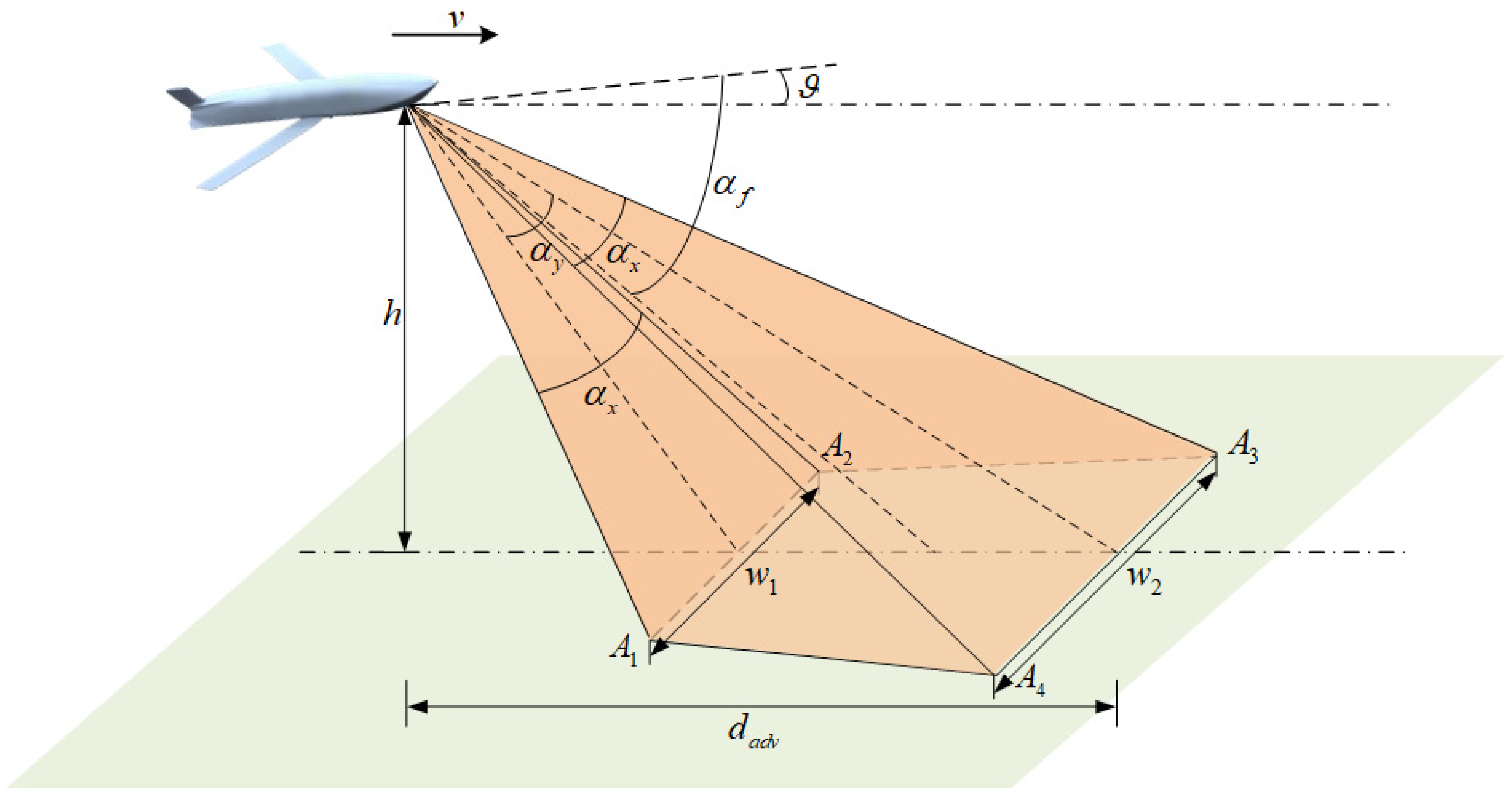
The camera model mounted on the fixed-wing UAV is shown in Figure 1. As depicted in Figure 1, a fixed-wing UAV flying at height $h$ acquires an image with the camera pointing forward-down, the corresponding trapezium area $A_1{A}_2{A}_3{A}_4$ is called the projected area, also called the camera footprint.

For conservative reasons and to ensure the quality of the photos, the bottom width of the camera footprint $w_1$ is defined as the sweep breadth of camera, which can be computed by:

$$w_1=\frac{2h\tan (\frac{{\alpha }_x}{2})}{\sin ({\alpha }_f-\vartheta +\frac{{\alpha }_y}{2})}$$

(1)

where ${\alpha }_x$ is the horizontal angle of view, ${\alpha }_y$ is the vertical angle of view, ${\alpha }_f$ is the front-mounted angle (the included angle between the bisector of ${\alpha }_y$ and UAV’s longitudinal axis), and $\vartheta$ is the pitch angle.

The zoom camera can vary the focal length $f$ to meet different task requirements. ${\alpha }_x$, ${\alpha }_y$ change as $f$ changes:

$$\{\begin{array}{l}{\alpha }_x=2\arctan (\frac{I_x}{2f})\\ {\alpha }_y=2\arctan (\frac{I_y}{2f})\end{array}$$

(2)

where $I_x$ and $I_y$ are image width and height respectively.

By Equations (1) and (2), we can conclude that camera footprint $w_1$ is a function of $h$, ${\alpha }_f$, $\vartheta$, $f$, $I_x$, $I_y$. The image width and height $I_x$, $I_y$ are constants, and when the fixed-wing UAV flies horizontally at cruise speed $v$, the front-mounted angle ${\alpha }_f$ and the pitch angle $\vartheta$ are usually set as constants. Therefore, the camera footprint $w_1$ is varied according to flight height $h$ and the focal length $f$, that is $w_1=g(h,f)$.

In path planning, a practical issue that is often overlooked is shooting advance distance $d_{adv}$, shown in Figure 1. $d_{adv}$ must be taken into account in waypoints generation. It can be computed by:

$$d_{adv}=\frac{h}{\tan ({\alpha }_f-\vartheta -\frac{{\alpha }_y}{2})}$$

(3)

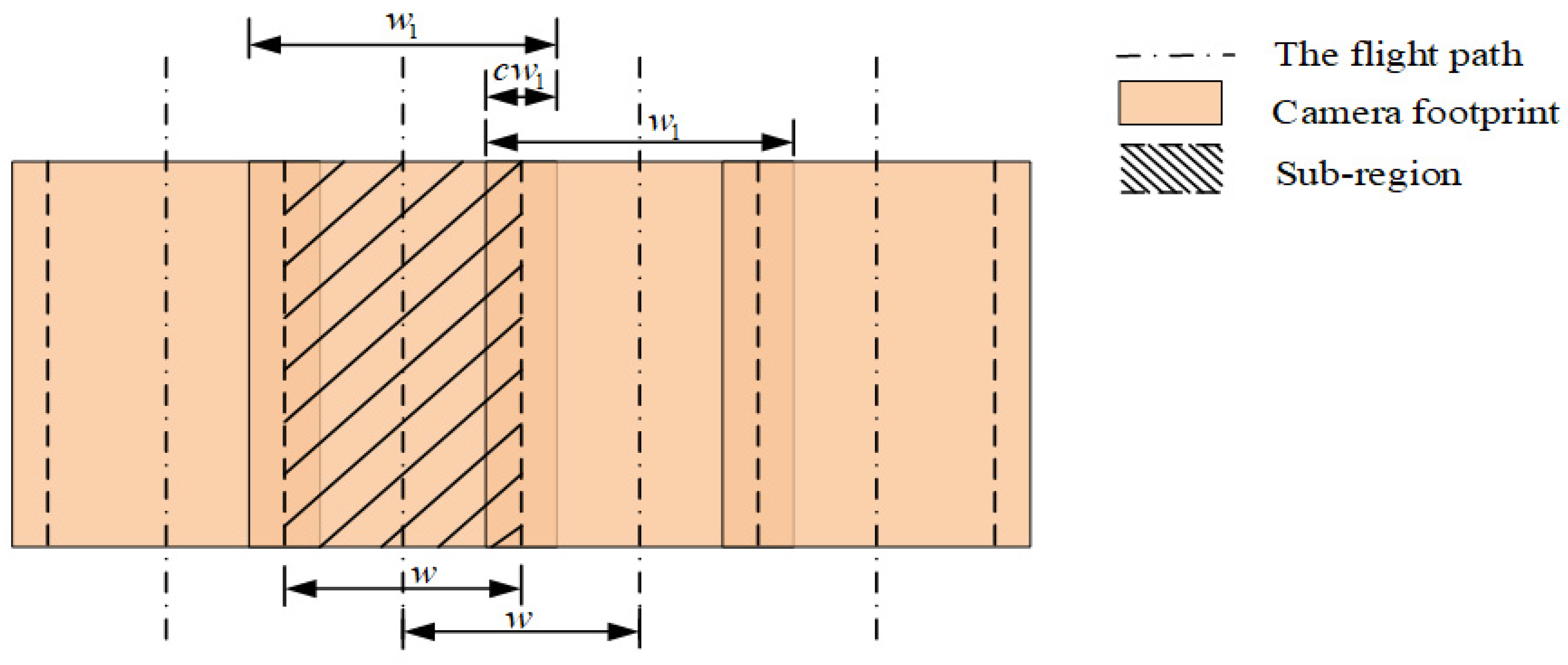
After the sweep breadth of camera $w_1$ is calculated, the region of interest can be completely covered by parallel paths at a certain distance $w$, which means the distance between two adjacent paths, as shown in Figure 2. In addition, $w$ also means the width of a sub-region. It can be obtained that $w=w_1(1-c)$, where $c\in (0,1)$ represents the overlap rate between two images. This overlap is generally necessary for photogrammetry. As depicted in Figure 2, the ROI can be divided into a set of parallel sub-regions in the width of $w$; once all these sub-regions are scanned, the entire ROI is completely covered.

As for the kinematic model of the fixed-wing UAV, it can be obtained according to the reference [34]:

$$\{\begin{array}{l}{F}_L\cos \delta =mg\\ F_L\sin \delta =\frac{m{v}^2}{R}\end{array}$$

(4)

where $F_L$ is the lift of the UAV, $\delta$ is the rolling angle of the UAV, $m$ is the mass and $R$ is the turning radius of the UAV, $g$ represents the acceleration of gravity, and $v$ is the instantaneous velocity of the UAV, $v\in [V_{\min },V_{\max }]$.

By Equation (4), the minimum turning radius of the fixed-wing UAV can be obtained as follows:

$$R_{\min }=\frac{V_{\min }^2}{g\tan \delta }$$

(5)

where $V_{\min }$ is the minimum flight speed of the UAV during the mission, $g$ is the gravitational acceleration, and $\delta$ is the rolling angle of the fixed-wing UAV.

The rolling angle $\delta$ represents the maneuverability of the fixed-wing UAV. It is not difficult to find that the minimum turning radius $R_{\min }$ is related to its maneuverability and turning speed.

Based on the above discussions, the specific coverage path planning problems studied in this paper are given as follows:

Problem 1.

For a convex polygon ROI, determine the best sweep direction of the UAV to reduce the number of turns.

Problem 2.

Considering the relationship between the minimum turning radius$R_{\min }$and the width of a sub-region$w$, design a turning strategy to shorten the path length of turns.

Problem 3.

Generating the waypoints for the fixed-wing UAV, ensure all sub-regions are searched, so that the ROI is entirely covered.

4. Materials and Methods

To solve the problems raised, the corresponding methods will be detailed in this section. Firstly, the coordinates of the ROI vertices are converted from the WGS-84 coordinate system to the local Cartesian coordinate system, which is also known as the East, North, Up (ENU) coordinate system. Secondly, the convex polygon of the ROI is rotated to find the minimum width direction, so as to determine the best sweep direction. Then, the convex polygon is divided into parallel polygonal sub-regions in the width of $w$, and the points where the UAV enters/leaves the sub-regions are computed. The turning strategy is determined by the relationship between the minimum turning radius $R_{\min }$ and the sub-region width $w$. Finally, the waypoints in the proposed interlaced back-and-forth flight pattern are generated and converted from the ENU coordinate system back to the WGS-84 coordinate system for the UAV field flight requirements. The flow chart of the CPP method proposed in the paper is shown in Figure 3.

4.1. Coordinate Conversion

In a practical photogrammetry mission, the only information of the ROI that can be obtained is the vertex coordinates in the WGS-84 coordinate system. Assuming the input vertices of the ROI are $Q_1,Q_2,\dots ,Q_N$ in turns, $N$ is the number of vertices, the coordinates of the i-th vertex $Q_i$, $i=1,2,\dots ,N$, are $({\gamma }_i,{\phi }_i,al{t}_i)$, where ${\gamma }_i$ and ${\phi }_i$ are the longitude and latitude of the vertex $Q_i$, and $al{t}_i$ is the altitude of the vertex $Q_i$. Since the vertices $Q_i$, $i=1,2,\dots ,N$ are defined in the WGS-84 coordinate system, which is a spherical coordinate system and inconvenient for UAV path planning, it is necessary to convert the coordinates of the ROI vertices from the WGS-84 coordinate system to the ENU coordinate system. In the ENU coordinate system, the origin is set by the user, the x-axis is pointing east, the y-axis is pointing north, and the z-axis is pointing up. To convert the coordinates from the WGS-84 coordinate system to the ENU coordinate system, the Earth-centered, Earth-fixed (ECEF) coordinate system is needed as a bridge. The coordinates of vertex $Q_i$, $i=1,2,\dots ,N$, are converted to coordinates that are in the ECEF coordinate system, then, they are converted to $E_i=(x_i^{ENU},y_i^{ENU},z_i^{ENU})$, $i=1,2,\dots ,N$ that are in the ENU coordinate system. The specific conversion formulas can be found in [26], which considered the Earth’s radius for higher accuracy.

Because the coverage path planning of the UAV in the following section is a two-dimensional path planning problem, only the information of the x-axis and y-axis is considered, vertices $E_i$ in the ENU coordinate system are set as $E_i=(x_i^{ENU},y_i^{ENU})$, $i=1,2,\dots ,N$, ignoring the z-coordinate.

Depending on the task and endurance of the fixed-wing UAV, the area of the ROI can be up to 4 km². We assume the vertices of the ROI are $Q_1$, $Q_2$, $Q_3$, $Q_4$ and $Q_5$ in the WGS-84 coordinate system. After coordinate conversion, the vertices are $E_1$, $E_2$, $E_3$, $E_4$ and $E_5$ in the ENU coordinate system, $E_1$ is set as the origin, as shown in Figure 4.

The coordinates of $Q_i$, $i=1,2,\dots ,5$, and $E_i$, $i=1,2,\dots ,5$, are given in

Table 1. Coordinates of the vertices.

Vertex	$(\mathit{\gamma },\mathit{\phi },\mathit{a}\mathit{l}\mathit{t})$	Vertex	$({\mathit{x}}_{}^{\mathit{E}\mathit{N}\mathit{U}},{\mathit{y}}_{}^{\mathit{E}\mathit{N}\mathit{U}})$
$Q_1$	(106.071582° E, 36.384018° N, 100 m)	$E_1$	(0 m, 0 m)
$Q_2$	(106.102668° E, 36.385275° N, 100 m)	$E_2$	(2789.13 m, 139.93 m)
$Q_3$	(106.097127° E, 36.402699° N, 100 m)	$E_3$	(2291.47 m, 2073.27 m)
$Q_4$	(106.085506° E, 36.404911° N, 100 m)	$E_4$	(1248.99 m, 2318.51 m)
Q5	(106.064360° E, 36.394924° N, 100 m)	$E_5$	(−647.90 m, 1210.22 m)

.

4.2. Sweep Direction Determination

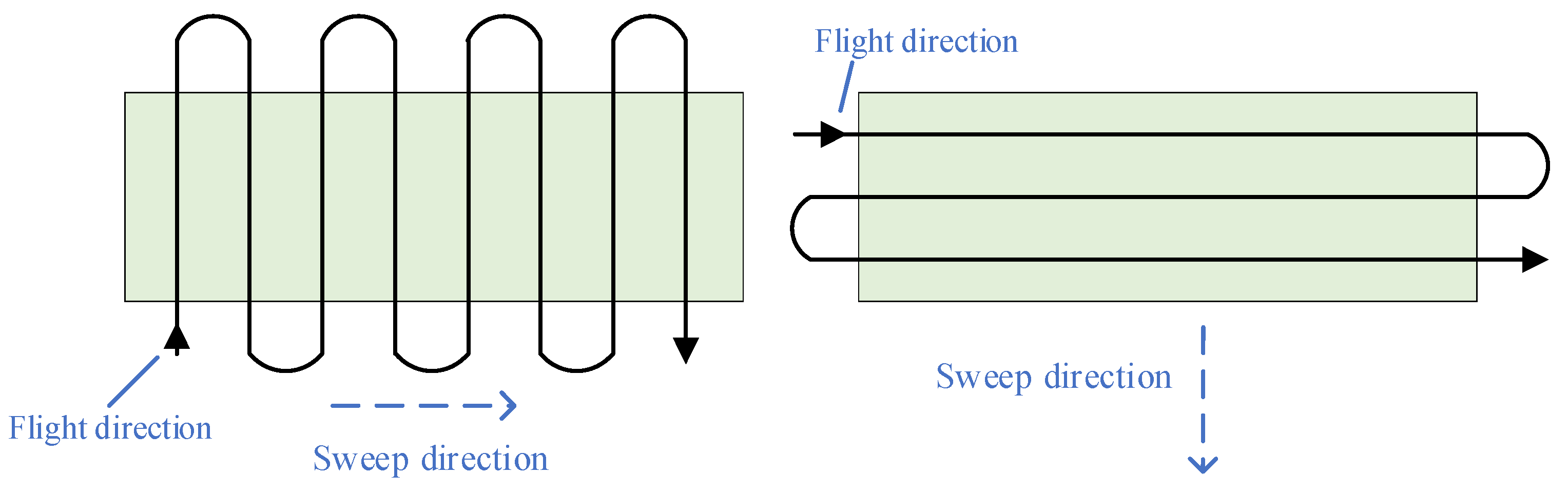
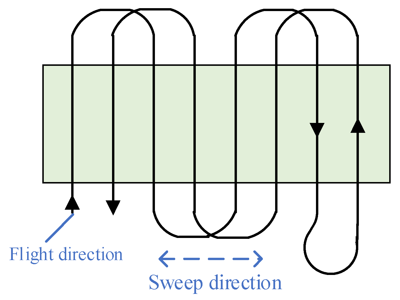
The sweep direction of the UAV plays a crucial role in the number of turning maneuvers when the back-and-forth (BF) flight pattern is utilized, as shown in Figure 5. As suggested by [35], the optimal sweep direction for coverage is parallel to the minimum width direction of the convex polygon. In this direction, the ROI can be covered with the smallest number of parallel paths, thus with the smallest number of turns.

In order to find the minimum width direction of the convex polygon of the ROI and determine the best sweep direction, a method based on rotation transformation is utilized. In the ENU coordinate system, the polygon of the ROI is rotated $\theta$, $\theta \in \left(0^{\circ },{360}^{\circ }\right]$ degrees counterclockwise about the origin. After rotation transformation, the new vertices of the polygon $E_{\theta i}=(x_{\theta i},y_{\theta i})$, $i=1,2,\dots ,N$ can be obtained:

$$E_{\theta i}{}^T=T·E_i{}^T=\left[\begin{array}{cc}\cos \theta & -\sin \theta \\ \sin \theta & \cos \theta \end{array}\right]·\left[\begin{array}{c}{x}_i^{ENU}\\ y_i^{ENU}\end{array}\right]$$

(6)

where $T$ is the rotational transfer matrix, $E_i$, $i=1,2,\dots ,N$, are the vertex coordinates in the ENU coordinate system before rotation transformation.

The vertex coordinates $E_{\theta i}=(x_{\theta i},y_{\theta i})$, $i=1,2,\dots ,N$ are computed for every degree of rotation. Set $l_{\theta }=\max x_{\theta i}-\min x_{\theta i}$, $\theta =1,2,\dots ,360$, $i=1,2,\dots ,N$. When $l_{\theta }=\min l_{\theta }$, we have ${\theta }_{\min }=\theta$. Then $P_i=(x_i{}^P,y_i{}^P)$, $i=1,2,\dots ,N$ can be obtained:

$$P_i{}^T=T_{\theta \min }·E_i{}^T=\left[\begin{array}{cc}\cos {\theta }_{\min }& -\sin {\theta }_{\min }\\ \sin {\theta }_{\min }& \cos {\theta }_{\min }\end{array}\right]·\left[\begin{array}{c}{x}_i^{ENU}\\ y_i^{ENU}\end{array}\right]$$

(7)

where $T_{\theta \min }$ is the rotational transfer matrix with ${\theta }_{\min }$, $E_i$, $i=1,2,\dots ,N$, are the vertex coordinates in the ENU coordinate system before rotation transformation.

For the polygon with vertices $P_i$, $i=1,2,\dots ,N$, its minimum width direction is parallel to the x-axis of the ENU coordinate system, so the optimal sweep direction of this polygon is parallel to the x-axis too, as depicted in Figure 6.

4.3. Polygon Decomposition

After the polygon of the ROI is converted to the polygon $P_1{P}_2\dots P_N$ whose minimum width direction is parallel to the x-axis, it is not difficult to find that the flight direction of the UAV should be perpendicular to the x-axis, as depicted in Figure 5. Therefore, the polygon is divided into polygonal sub-regions parallel to the y-axis, and the points where the UAV enters and leaves the sub-regions can be computed.

In this paper, the span coefficient of the fixed-wing UAV is first proposed, and is defined as follows:

$$\lambda =ceil(\frac{2R_{\min }}{w})$$

(8)

where function ceil represents rounding up, $R_{\min }$ is the minimum turning radius of the fixed-wing UAV, $w$ is the sub-region width as defined in Section 3.

The number of sub-regions can be calculated as follows:

$$n=\lambda ·ceil(\frac{x_{\max }-x_{\min }}{\lambda w})$$

(9)

where $\lambda$ is the span coefficient, $w$ is the sub-region width, $x_{\max }=\max x_i^P$, $x_{\min }=\min x_i^P$, $i=1,2,\dots ,N$ are the maximum and minimum x-coordinate values of the vertices $P_i$, $i=1,2,\dots ,N$.

The border between the j-th sub-region and (j+1)-th sub-region can be computed by Equation (10).

$$x_{bj}=x_{\min }+jw, j=1,2,\dots ,n-1$$

(10)

where $x_{\min }$ is minimum x-coordinate values of the vertices $P_i$, $i=1,2,\dots ,N$, $w$ is the sub-region width, and $n$ is the number of sub-regions.

Then, the j-th sub-region can be represented as follows:

$$\{\begin{array}{l}x\ge x_{\min }+(j-1)w\\ x\le x_{\min }+jw\end{array}, j=1,2,\dots ,n$$

(11)

The x-coordinate value of path that the UAV passes in the j-th sub-region can be computed as follows:

$$x_j=\frac{x_{\min }+(j-1)w+x_{\min }+jw}{2}=x_{\min }+(j-0.5)w, j=1,2,\dots ,n$$

(12)

The expressions of the edges of the convex polygon $P_1{P}_2\dots P_N$ can be written as follows:

$$\{\begin{array}{l}y=k_{i}x+b_i\\ x_{i\min }<x<x_{i\max }\\ y_{i\min }<y<y_{i\max }\end{array}, i=1,2,\dots ,N$$

(13)

where $k_i$ is the slope of the i-th edge, $b_i$ is the y-intercept of the i-th edge, $x_{i\min }$ and $x_{i\max }$ are the minimum and maximum x-coordinate values of the i-th edge, $y_{i\min }$ and $y_{i\max }$ are the minimum and maximum y-coordinate values of the i-th edge.

Since the polygon region $P_1{P}_2\dots P_N$ and sub-regions have been modeled, the minimum and maximum y-coordinate values of the vertices of each sub-region can be calculated. Let the set of y-coordinates values of all vertices in the j-th subregion be $U_j$, $j=1,2,\dots ,n$. The relationship between edges of the polygon $P_1{P}_2\dots P_N$ and sub-regions are discussed and the set of $U_j$ are computed according to Equations (11) and (13).

(i)

When the minimum and maximum x-coordinate values of the i-th edge of the polygon $P_1{P}_2\dots P_N$ satisfy the following inequalities:

$$\{\begin{array}{l}{x}_{\min }+(j-1)w<x_{i\max }<x_{\min }+jw\\ x_{i\min }<x_{\min }+(j-1)w\end{array}$$

(14)

that means the i-th edge passes through the left border of the j-th subregion. Therefore, $k_i{x}_{i\max }+b_i$ and $k_i{x}_{\min }+k_i(j-1)w+b_i$ should be included in the set of $U_j$, that is $\left\{k_i{x}_{i\max }+b_i,k_i{x}_{\min }+k_i(j-1)w+b_i\right\}\subset U_j$.

(ii)

When the minimum and maximum x-coordinate values of the i-th edge of the polygon $P_1{P}_2\dots P_N$ satisfy the following inequalities:

$$\{\begin{array}{l}{x}_{\min }+(j-1)w<x_{i\min }<x_{\min }+jw\\ x_{i\max }>x_{\min }+jw\end{array}$$

(15)

that means the i-th edge passes through the right border of the j-th subregion. Hence, $k_i{x}_{i\min }+b_i$ and $k_i{x}_{\min }+k_{i}jw+b_i$ should be included in the set of $U_j$, that is $\left\{k_i{x}_{i\min }+b_i,k_i{x}_{\min }+k_{i}jw+b_i\right\}\subset U_j$.

(iii)

When the minimum and maximum x-coordinate values of the i-th edge of the polygon $P_1{P}_2\dots P_N$ satisfy the following inequalities:

$$\{\begin{array}{l}{x}_{i\min }\le x_{\min }+(j-1)w\\ x_{i\max }\ge x_{\min }+jw\end{array}$$

(16)

that means the i-th edge passes through the left and right border of the j-th subregion, both. So, $k_i{x}_{\min }+k_i(j-1)w+b_i$ and $k_i{x}_{\min }+k_{i}jw+b_i$ should be included in the set of $U_j$, that is $\left\{k_i{x}_{\min }+k_i(j-1)w+b_i,k_i{x}_{\min }+k_{i}jw+b_i\right\}\subset U_j$.

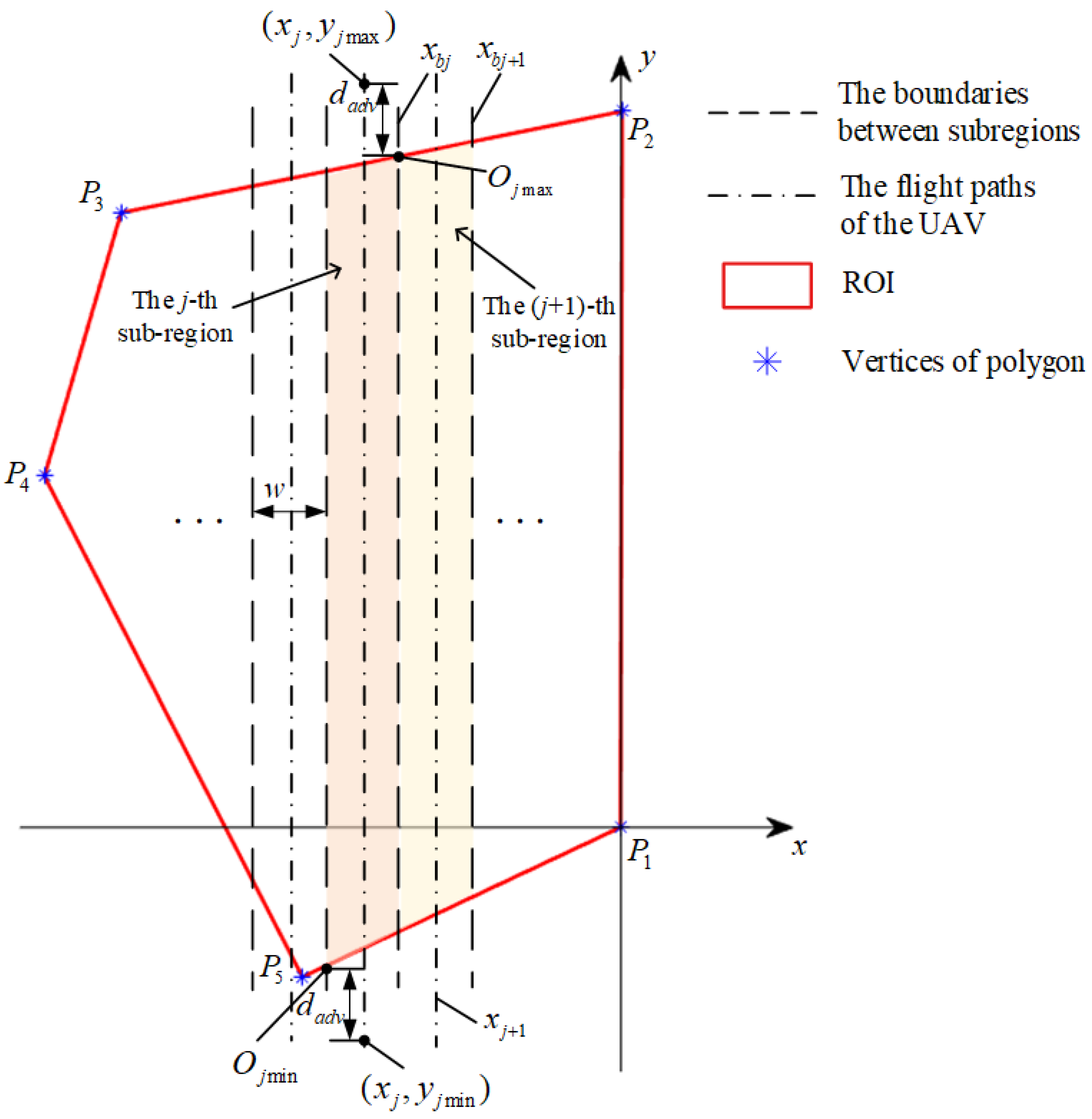
Based on the discussions and calculations above, the set of $U_j$, $j=1,2,\dots ,n$, can be obtained. Let the minimum and maximum values of the set of $U_j$ be $O_{j\min }$ and $O_{j\max }$, respectively, it can be obtained $O_{j\min }=\min U_j$, $O_{j\max }=\max U_j$, $j=1,2,\dots ,n$. Considering the shooting advance distance $d_{adv}$, the y-coordinate value of the UAV enters/leaves the j-th subregion is $y_{j\max }$/$y_{j\min }$, where $y_{j\max }=O_{j\max }+d_{adv}$, $y_{j\min }=O_{j\min }-d_{adv}$, as shown in Figure 7. Combine with $x_j$ computed by Equation (10), the waypoints of the UAV entering or leaving the j-th sub-region are determined as $(x_j,y_{j\max })$ or $(x_j,y_{j\min })$.

4.4. Analysis of the Turning Strategy

To shorten the path length of turns, a novel turning strategy considering the relationship between the minimum turning radius $R_{\min }$ and the width of a sub-region $w$ is proposed and compared with the traditional method.

Firstly, the traditional turning strategy is introduced. In a traditional turning scenario, the ROI is swept line by line, after a sub-region is scanned, the fixed-wing UAV will make a turn maneuver to the next sub-region adjacent. And the path of turning is usually a Dubins path. Dubins path is the shortest path connecting two points in a two-dimensional plane, with prescribed initial and terminal direction of the velocity [36]. A typical turning scenario when $2R_{\min }>w$ by traditional turning strategy is depicted in Figure 8, which is an RLS type of Dubins path; R represents turning clockwise while L means turning counterclockwise, and S stands for a straight line.

Let the first path length of turn be $L_{t1}$, and it can be obtained as follows:

$$L_{t1}=\alpha R_{\min }$$

(17)

where $\alpha$ is the angle of the arc $L_{t1}$, $\alpha =\arccos (w/2R_{\min })$, $R_{\min }$ is the minimum turning radius of the fixed-wing UAV.

Let the second path length of turn be $L_{t2}$, it can be obtained as follows:

$$L_{t2}=(\frac{3\pi }{2}-\beta )R_{\min }=(\pi +\alpha )R_{\min }$$

(18)

where $\beta$ is the angle of the arc $L_{t2}$, $\beta =\pi /2-\alpha$, and $R_{\min }$ is the minimum turning radius of the fixed-wing UAV.

Let the straight path length of turn be $L_s$, it can be calculated as follows:

$$L_s=\sqrt{{(2R_{\min })}^2-{(w+R_{\min }-R_{\min })}^2}=\sqrt{4R_{\min }^2-w^2}$$

(19)

where $R_{\min }$ is the minimum turning radius of the fixed-wing UAV and $w$ is the width of a sub-region.

The total curve path length of a turn in traditional turning strategy is denoted as $L_t$, and it is defined as follows:

$$L_t=L_{t1}+L_{t2}=(\pi +2\alpha )R_{\min }$$

(20)

The total path length of a turn in traditional turning strategy is denoted as $L_{sum}$, it is defined as follows:

$$L_{sum}=L_{t1}+L_{t2}+L_s=(\pi +2\alpha )R_{\min }+\sqrt{4R_{\min }^2-w^2}$$

(21)

As shown in Figure 8, when $2R_{\min }$ is larger than $w$, there will be a wide turning maneuver between two adjacent paths by the traditional turning strategy. These wide turns cost more energy and lead to longer turning distances. To solve this problem, a novel interlaced turning strategy is presented in the paper.

In the interlaced turning strategy, after a sub-region is scanned, the fixed-wing UAV will make a turn to the next sub-region, which is adjacent or apart by several sub-regions, depending on the relationship between $R_{\min }$ and $w$. The interlaced turning scenario is shown in Figure 9, which is an LSL type of Dubins path, L represents turning counterclockwise, and S stands for a straight line.

Let the first curve path length of turn by the interlaced turning strategy be $L_{t1}{}^{\prime }$, and it can be obtained as follows:

$$L_{t1}{}^{\prime }=\frac{\pi }{2}{R}_{\min }$$

(22)

where $R_{\min }$ is the minimum turning radius of the fixed-wing UAV.

Let the second curve path length of turn by the interlaced turning strategy be $L_{t2}{}^{\prime }$, it can be obtained as follows:

$$L_{t2}{}^{\prime }=\frac{\pi }{2}{R}_{\min }$$

(23)

where $R_{\min }$ is the minimum turning radius of the fixed-wing UAV.

Let the straight path length of turn by the interlaced turning strategy be $L_s{}^{\prime }$, it can be calculated as follows:

$$L_s{}^{\prime }=\lambda w-2R_{\min }$$

(24)

where $\lambda$ is the span coefficient defined in Equation (6), $w$ is the width of a sub-region, and $R_{\min }$ is the minimum turning radius of the fixed-wing UAV.

The total curve path length of a turn by the interlaced turning strategy is denoted as $L_t{}^{\prime }$, and it is defined as follows:

$$L_t{}^{\prime }=L_{t1}{}^{\prime }+L_{t2}{}^{\prime }=\pi R_{\min }$$

(25)

The total path length of a turn in the interlaced turning strategy is denoted as ${L^{\prime }}_{sum}$, it is defined as follows:

$${L^{\prime }}_{sum}=L_{t1}{}^{\prime }+L_{t2}{}^{\prime }+L_s{}^{\prime }=(\pi -2)R_{\min }+\lambda w$$

(26)

Through comparative analyses of the traditional and proposed turning strategies, the following important results can be obtained:

Result 1.

The total curve path length of a turnby the interlaced turning strategy is always shorter than that by the traditional turning strategy when $2R_{\min }>w$, that is$\lambda >1$.

Proof. 

Equation (20) minus Equation (25), we can obtain $L_t-L_t{}^{\prime }=2\alpha R_{\min }$. Since $\alpha >0$, $R_{\min }>0$, it is obvious that $L_t-L_t{}^{\prime }>0$, thus $L_t{}^{\prime }<L_t$. □

Result 2.

The straight path length of a turn by the interlaced turning strategy is always shorter than that by the traditional turning strategy when$2R_{\min }/w>1.25$.

Proof. 

Square Equation (19), we have:

$$L_s^2=4R_{\min }^2-w^2$$

(27)

Then, square Equation (24), we have:

$$L_s{{}^{\prime }}^2={(\lambda w-2R_{\min })}^2={\lambda }^2{w}^2-4\lambda w{R}_{\min }+4R_{\min }^2$$

(28)

Let Equation (27) minus Equation (28), it can be obtained that:

$$L_s^2-L_s{{}^{\prime }}^2=-(1+{\lambda }^2)w^2+4\lambda w{R}_{\min }$$

(29)

If we have $L_s^{}>L_s{}^{\prime }$, the following condition needs to be met according to Equation (29):

$$-(1+{\lambda }^2)w^2+4\lambda w{R}_{\min }>0$$

(30)

that can be converted to in Equation (31) as follows:

$$\frac{2R_{\min }}{w}>\frac{{\lambda }^2+1}{2\lambda }$$

(31)

where $\lambda$ is defined in Equation (8), $\lambda =ceil(\frac{2R_{\min }}{w})$.

Denote the left-hand side of the inequality (31) as $f_1(x)=\frac{2R_{\min }}{w}$, where $x=\frac{2R_{\min }}{w}$, $x>1$. Denote the right-hand side of the inequality (31) as $f_2(x)=\frac{{\lambda }^2+1}{2\lambda }$, where $x=\frac{2R_{\min }}{w}$, $x>0$, $\lambda =ceil(x)$.

When $x=1.25$, we have $f_1(x)=1.25$, $f_2(x)=\frac{2^2+1}{2\times 2}=1.25$, that is $f_1(x)=f_2(x)$.

When $1<x<1.25$, we have $1<f_1(x)<1.25$, $f_2(x)=\frac{2^2+1}{2\times 2}=1.25$, so $f_1(x)<f_2(x)$.

When $1.25<x\le 2$, we have $1.25<f_1(x)\le 2$, $f_2(x)=\frac{2^2+1}{2\times 2}=1.25$, so $f_1(x)>f_2(x)$.

When $x>2$, we assume $x=t$, $t\in \left(N,N+1\right]$, where $N$ is a positive integer and $N\ge 2$. It can be obtained that:

$$f_1(x)=t>N$$

(32)

Since $\lambda =ceil(x)=ceil(t)=N+1$, we have:

$$f_2(x)=\frac{{\lambda }^2+1}{2\lambda }=\frac{{(N+1)}^2+1}{2(N+1)}=\frac{N+1}{2}+\frac{1}{2(N+1)}$$

(33)

Because $N$ is a positive integer and $N\ge 2$, it can be obtained that:

$$f_2(x)=\frac{N+1}{2}+\frac{1}{2(N+1)}<\frac{N}{2}+\frac{1}{2}+\frac{1}{6}<\frac{N}{2}+1<\frac{N}{2}+\frac{N}{2}=N$$

(34)

By inequality (32) and (34), we have $f_1(x)>f_2(x)$ when $x>2$.

Therefore, it can be obtained that $f_1(x)>f_2(x)$, when $x>1.25$. So, the inequality (30) holds, we have $L_s^{}>L_s{}^{\prime }$ if $2R_{\min }/w>1.25$. □

Result 3.

The total path length of a turn by the interlaced turning strategy is always shorter than that by the traditional turning strategy when$2R_{\min }/w>1.25$.

Proof. 

From Equation (26), we have the total path length of a turn in the interlaced turning strategy, that is ${L^{\prime }}_{sum}=L_{t1}{}^{\prime }+L_{t2}{}^{\prime }+L_s{}^{\prime }=L_t{}^{\prime }+L_s{}^{\prime }$, and we have the total path length of a turn in traditional turning strategy, that is $L_{sum}=L_{t1}+L_{t2}+L_s=L_t+L_s$ according to Equation (21). Result 1 indicates $L_t{}^{\prime }<L_t$ while Result 2 states $L_s{}^{\prime }<L_s^{}$ in the condition of $2R_{\min }/w>1.25$. Hence it can be concluded that ${L^{\prime }}_{sum}<L_{sum}$ when $2R_{\min }/w>1.25$. □

Result 4.

The total path length of a turn by the interlaced turning strategy may be longer or shorter than that by the traditional turning strategy when$1<2R_{\min }/w\le 1.25$.

Proof. 

From Equation (26), we have the total path length of a turn in the interlaced turning strategy, that is ${L^{\prime }}_{sum}=L_{t1}{}^{\prime }+L_{t2}{}^{\prime }+L_s{}^{\prime }=L_t{}^{\prime }+L_s{}^{\prime }$, and we have the total path length of a turn in traditional turning strategy, that is $L_{sum}=L_{t1}+L_{t2}+L_s=L_t+L_s$ according to Equation (21). Result 1 indicates $L_t{}^{\prime }<L_t$. However, $L_s{}^{\prime }>L_s^{}$ when $1<2R_{\min }/w\le 1.25$. Therefore, the relationship between ${L^{\prime }}_{sum}$ and $L_{sum}$ must be calculated by Equations (21) and (26). □

Remark 1.

When$0<2R_{\min }/w\le 1$,$\lambda =1$, the traditional turning strategy degenerates to the interlaced turning strategy presented in this paper.

4.5. Waypoints Generation

The aim of coverage path planning is path generation. For the UAV, the paths are generated through waypoints, because the UAV flies according to input waypoint instructions. Based on the above discussions, we have found the optimal sweep direction, and the waypoints where the UAV enters or leaves each sub-region. Above all, the interlaced turning strategy has been fully studied. It is time to determine all waypoints according to the proposed turning strategy and link them together in sequence.

Remark 2.

The waypoints are firstly generated for the polygon region$P_1{P}_2\dots P_N$for convenience, then, the coordinates of the waypoints are transformed back to the ROI$E_1{E}_2\dots E_N$by the inverse rotational transfer matrix$T^T=\left[\begin{array}{cc}\cos \theta & \sin \theta \\ -\sin \theta & \cos \theta \end{array}\right]$.

When $\lambda =1$, that is $0<2R_{\min }/w\le 1$, the coverage flight pattern with the interlaced turning strategy is the same as the conventional BF flight pattern, just as shown in Figure 5. However, when $\lambda \ge 2$, the flight pattern is quite different. The UAV will sweep the ROI $\lambda$ times; after the ROI has been swept once, the UAV makes a turn for the next sweep. This is due to the interlaced turning strategy. We have named this new type of flight pattern as the interlaced BF pattern. A typical coverage path in an interlaced BF flight pattern when $\lambda =2$ is shown in Figure 10.

It can be obtained that the number of sub-regions that the UAV passes through in each sweep is:

$$n_{\lambda }=ceil(\frac{x_{\max }-x_{\min }}{\lambda w})$$

(35)

where $\lambda$ is the span coefficient defined in Equation (8), $w$ is the sub-region width, $x_{\max }=\max x_i^P$, $x_{\min }=\min x_i^P$, $i=1,2,\dots ,N$ are the maximum and minimum x-coordinate values of the vertices $P_i$, $i=1,2,\dots ,N$.

The number of the UAV making a turn to the next sweep can be obtained as $n_t=\lambda -1$.

Assuming the start point of the UAV is $S_{start}=(x_{\min }+0.5w,y_{1\max })$, at the upper left of the polygon region $P_1{P}_2\dots P_N$. Let the set of sub-regions that the UAV passes through in the p-th ($p=1,2,\dots ,\lambda$) sweep be $J_p$, it can be obtained as follows:

$$J_p=\left\{j\right|j=p+q\lambda ,q=0,1,\dots ,n_{\lambda }-1\}$$

(36)

where $j$ represents the serial number of the sub-region.

Combining the set of $J_p$ with the waypoints of the UAV entering and leaving the j-th sub-region obtained in Section 4.3, the waypoints of the UAV in each sweep are determined. The waypoints connecting each sweep are discussed below:

(i)

When $n_{\lambda }$ is odd, the UAV will make a turn to the next sweep at the bottom right of the polygon region $P_1{P}_2\dots P_N$ when it sweeps from the start point $S_{start}$. The start point $S_{sp}$ and end point $S_{ep}$ of the p-th ($p=1,2,\dots ,n_t$) turn to the next sweep are determined as follows:

$$S_{sp}=\{\begin{array}{l}(x_{\min }+(p^{\prime }-0.5)w,y_{p^{\prime }\min }), p is odd\\ (x_{\min }+(p-0.5)w,y_{p\max }), p is even\end{array},S_{ep}=\{\begin{array}{l}(x_{\min }+(p^{\prime }+0.5)w,y_{(p^{\prime }+1)\min }), p is odd\\ (x_{\min }+(p+0.5)w,y_{(p+1)\max }), p is even\end{array}$$

(37)

where $x_{\min }=\min x_i^P$, $i=1,2,\dots ,N$ is the minimum x-coordinate values of polygon $P_1{P}_2\dots P_N$, $p^{\prime }=p+(n_{\lambda }-1)\lambda$, $w$ is the sub-region width, $y_{p^{\prime }\min }$ represents the minimum y-coordinate value of the UAV waypoint before entering the $p^{\prime }$-th subregion, $y_{p\max }$ represents the maximum y-coordinate value of the UAV waypoint before entering the $p$-th subregion.

(ii)

When $n_{\lambda }$ is even, the UAV will make a turn to the next sweep at the upper right of the polygon region $P_1{P}_2\dots P_N$ when it sweeps from the start point $S_{start}$. The start point $S_{sp}$ and end point $S_{ep}$ of the p-th ($p=1,2,\dots ,n_t$) turn to the next sweep are determined as follows:

$$S_{sp}=\{\begin{array}{l}(x_{\min }+(p^{\prime }-0.5)w,y_{p^{\prime }\max }), p is odd\\ (x_{\min }+(p-0.5)w,y_{p\max }), p is even\end{array},S_{ep}=\{\begin{array}{l}(x_{\min }+(p^{\prime }+0.5)w,y_{(p^{\prime }+1)\max }), p is odd\\ (x_{\min }+(p+0.5)w,y_{(p+1)\max }), p is even\end{array}$$

(38)

where $x_{\min }=\min x_i^P$, $i=1,2,\dots ,N$ is the minimum x-coordinate values of polygon $P_1{P}_2\dots P_N$, $p^{\prime }=p+(n_{\lambda }-1)\lambda$, $w$ is the sub-region width, $y_{p^{\prime }\max }$ represents the maximum y-coordinate value of the UAV waypoint before entering the $p^{\prime }$-th subregion, $y_{p\max }$ represents the maximum y-coordinate value of the UAV waypoint before entering the $p$-th subregion.

Connect all the waypoints in sequence, and the final waypoints of the UAV are obtained. These waypoints are firstly transformed back to the ROI $E_1{E}_2\dots E_N$ by the inverse rotational transfer matrix $T^T$. Then, they are converted from the ENU coordinate system to the WGS-84 coordinate system for the practical requirements.

At the end of this section, the pseudocode of the waypoint generation is given as Algorithm 1.

Algorithm 1. Waypoint generation with interlaced BF flight pattern

1: Input: $Q_1,Q_2,\dots ,Q_N$, the vertex coordinates of ROI in the WGS-84 coordinate system

2: % Step 1. Coordinate conversion 3: for i = 1 to N do 4:   Convert $Q_i$ to $W_i$% to the ECEF coordinate system 5: end for 6: for i = 1 to N do 7:  Convert $W_i$ to $E_i$% to the ENU coordinate system 8: end for 9: % Step 2. Find the optimal sweep direction 10: $l=\max x_i-\min x_i$% Initialize 11: for $\theta$ = 1 to 360 do 12.   for i = 1 to N do 13.     Calculate $E_{\theta i}$ using Equation (4) 14.   end for 15.   $l_{\theta }=\max x_{\theta i}-\min x_{\theta i}$ 16.   if $l_{\theta }<l$ then 17.     $l=l_{\theta }$, ${\theta }_{\min }=\theta$ 18. end if 19. end for 20. for i = 1 to N do 21.   Calculate $P_i$ using Equation (5) 22. end for 23. % Step 3. Polygon decomposition and waypoints determination 24. Calculate n using Equation (7) % the number of sub-regions 25. for j = 1 to n do 26.   Calculate the set of $U_j$ by Equations (9) and (11) 27.   $O_{j\min }=\min U_j$, $O_{j\max }=\max U_j$ 28.   $y_{j\max }=O_{j\max }+d_{adv}$, $y_{j\min }=O_{j\min }-d_{adv}$ 29.   Calculate $x_j$ using Equation (10) 30. end for 31. % Step 4. Waypoints connecting according to interlaced BF pattern 32. Calculate $\lambda$ using Equation (6) 33. Calculate $n_{\lambda }$ using Equation (30) % the number of sub-regions in each sweep 34. for p = 1 to $\lambda$ do 35.   Calculate the set of $J_p$ by Equations (30) 36.   if $p\le n_t$ then 37.     if $n_{\lambda }$ is odd then 38.       Calculate $S_{sp}$ and $S_{ep}$ by Equation (32) 39.     else % $n_{\lambda }$ is even 40.       Calculate $S_{sp}$ and $S_{ep}$ by Equation (33) 41.     end if 42.   end if 43. end for 44. Sort $x_j$, $y_{j\max }$, $y_{j\min }$, $S_{sp}$, $S_{ep}$ 45. % Step 5. Coordinate conversion 46. Convert all waypoints by $T^T$% the inverse rotational transfer matrix 47. Convert all waypoints to WGS-84 coordinate system 48. Output: Waypoints in the WGS-84 coordinate system.

5. Simulations

In this section, to verify the effectiveness of the proposed interlaced BF coverage flight pattern, three groups of simulation experiments that compared the interlaced BF coverage with the traditional BF pattern are given. For the purpose of discussing the influence of the relationship between the minimum turning radius and the sub-region width defined in Section 3 on the results, we have $\lambda =2$ in the first group of experiments, and $\lambda =3$ in the second group of experiments. Finally, a group of experiments are used to demonstrate the conventional pattern is the same as the proposed one when $\lambda =1$.

The important input parameters of the experiments are summarized in

Table 2. The input parameters of the experiments.

Vertex of the ROI	Group of Experiments	${\mathit{V}}_{\mathit{t}\mathit{u}\mathit{r}\mathit{n}}(\mathbf{m}/\mathbf{s})$	$\mathit{\delta }$$\left({}^{\circ }\right)$	${\mathit{R}}_{\mathbf{min}}\left(\mathbf{m}\right)$	${\mathit{w}}_1\left(\mathbf{m}\right)$	$\mathit{c}$	$\mathit{w}$	$\mathit{\lambda }$
(106.071582° E, 36.384018° N, 100 m) (106.102668° E, 36.385275° N, 100 m) (106.097127° E, 36.402699° N, 100 m) (106.085506° E, 36.404911° N, 100 m) (106.064360° E, 36.394924° N, 100 m)	1	20	19	120	300	50%	150	2
	2	20	15	150	300	60%	120	3
	3	10	15	40	300	50%	150	1

, where $V_{turn}$ is the speed of turning, $\delta$ represents the roll angle of the fixed-wing UAV when making a turning maneuver, $R_{\min }$ is the minimum turning radius, $w_1$ is the sweep breadth of camera, $c$ is the overlap rate, $w$ is the width of a sub-region, and $\lambda$ is the span coefficient.

In the first group of simulations, refer to [34], the task is executed at a height of 300 m, the sweep breadth of camera $w_1$ is 300 m, the maximum flight speed $V_{\max }$, minimum flight speed $V_{\min }$, and cruise speeds are 25 m/s, 20 m/s, and 22 m/s, respectively. When the UAV flies in straight lines, the average speed is around 23 m/s, while the speed of turning is 20 m/s. Roll angle $\delta$ is set as 19 degrees. And the minimum turning radius $R_{\min }$ is calculated by Equation (5), $R_{\min }=120$ m. For a real and practical case of photogrammetry that uses SFM algorithm, the overlap between adjacent images is at least 45%. We have the overlap rate 50% in this simulation, that is $c=0.5$. Then, the width of a sub-region $w$ can be obtained, $w=w_1(1-c)=300\ast (1-0.5)=150$ m, and the span coefficient $\lambda =2$ by Equation (8). Furthermore, the shooting advance distance $d_{adv}$ is 100 m. The ROI is shown in Figure 4. 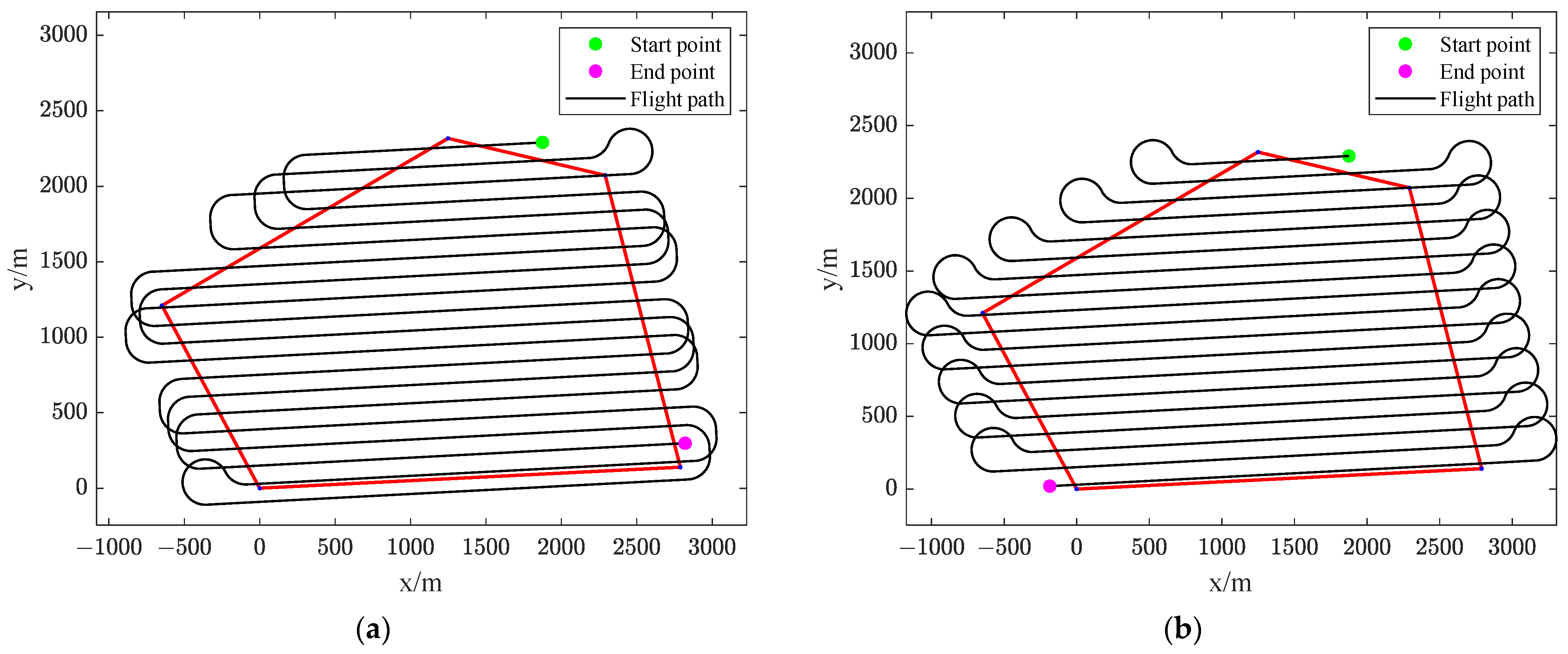Figure 11a shows the coverage path that is generated by the proposed interlaced BF flight pattern, and the path that is generated by traditional BF pattern is shown in Figure 11b. In Figure 11a, it can be seen that the UAV sweeps the ROI twice; after the ROI has been swept once, the UAV makes a turn for the next sweep. By contrast, the UAV sweeps the ROI line by line in a conventional BF pattern as shown in Figure 11b.

The number of turns, path length, and flight time of coverage path generated by different flight patterns when $\lambda =2$ are shown in

Table 3. Path comparison of different flight pattern when $\lambda =2$.

Path Parameters	Interlaced BF Pattern	Traditional BF Pattern	Percentage of Improvement
Number of turns	15	15	0%
The curve path length of turns(m)	5869.8	8879.3	33.89%
The straight path length of turns(m)	1027.3	2810.2	63.44%
The total path length of turns(m)	6897.1	11,689.5	41.00%
The total path length(m)	53,158.0	56,950.7	6.66%
Flight time(s)	2356.2	2552.4	7.69%

. The number of turns is the same in the interlaced BF pattern and the traditional BF pattern. However, the total path length of turns in the proposed interlaced BF pattern is greatly reduced, by 41.00% specifically. In addition, both the curve path and straight path length of turns in the interlaced BF pattern are shorter than that in the traditional BF pattern, which are consistent with Result 1 and Result 2. As for the total path length, it is reduced by 6.66% using the novel flight pattern, and more than 3 min of flight time are saved correspondingly. The percentage of the improvement of path saving and flight efficiency by the proposed method are shown in the right column of Table 3.

In the second group of simulations, the average speed when flying in straight lines is 23 m/s, the speed of turning is 20 m/s, the flight height is 300 m, the sweep breadth of the camera $w_1$ is 300 m, the shooting advance distance $d_{adv}$ is 100 m, which are similar to the first group of simulations. Differently, the overlap rate required is 60%, that is $c=0.6$ and the width of a sub-region $w$ can be calculated, $w=w_1(1-c)=300\ast (1-0.6)=120$ m. Moreover, the roll angle $\delta$ is set as 15 degrees, and the minimum turning radius $R_{\min }$ is calculated by Equation (5), $R_{\min }=150$ m. Then, it can be obtained that the span coefficient $\lambda =3$ according to Equation (8). 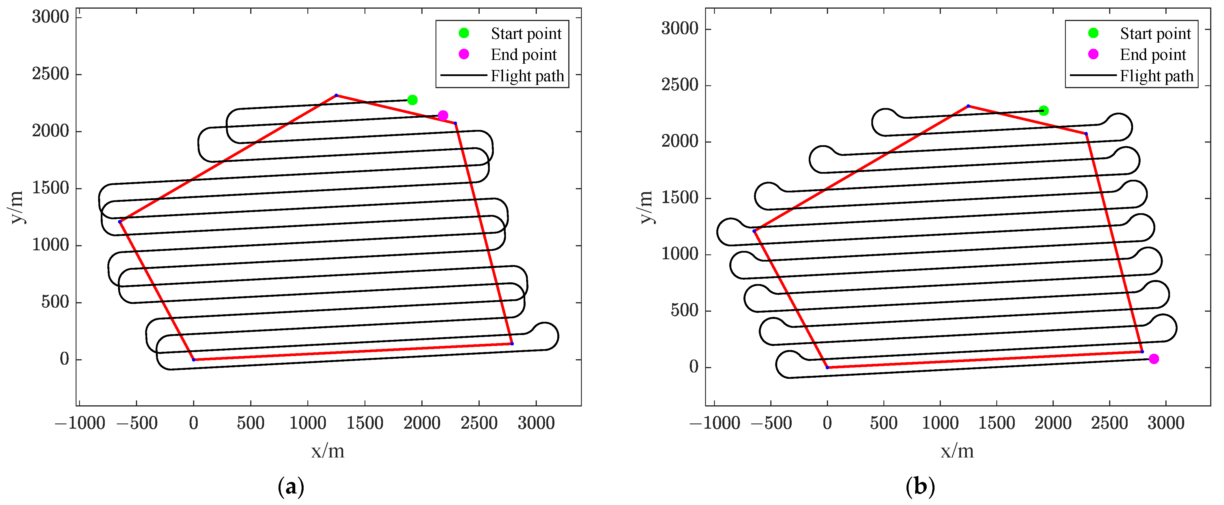Figure 12a shows the coverage path that is generated by the proposed interlaced BF flight pattern while Figure 12b shows the path generated by the traditional BF pattern. In Figure 12a, it can be seen that the UAV sweeps the ROI three times; after the ROI has been swept once, the UAV makes a turn for the next sweep. In the traditional BF pattern, however, the UAV sweeps the ROI line by line, as shown in Figure 12b.

The path parameters of the coverage path generated by different flight patterns when $\lambda =3$ are shown in

Table 4. Path comparison of different flight pattern when $\lambda =3$.

Path Parameters	Interlaced BF Pattern	Traditional BF Pattern	Percentage of Improvement
Number of turns	19	18	−5.56%
The curve path length of turns(m)	9649.3	14,743.3	34.55%
The straight path length of turns(m)	1569.8	4949.1	68.28%
The total path length of turns(m)	11,219.1	19,692.4	43.03%
The total path length(m)	70,105.6	74,002.8	5.27%
Flight time(s)	3121.2	3345.9	6.72%

. The number of turns in the interlaced BF pattern is more than that in the traditional BF pattern. However, the total path length of turns in the proposed interlaced BF pattern is reduced by more than 40%. In addition, both the curve path and straight path length of turns in the interlaced BF pattern are shorter than that in the traditional BF pattern, which is consistent with Result 1 and Result 2. As for the total path length, it is reduced by 5.27% using the interlaced BF flight pattern, and 3 min 45 s of flight time are saved correspondingly. For the same ROI, it is worth noting that the total path length of turns decreases more with the increase of $\lambda$($\lambda \ge 2$), 4792.4 m when $\lambda =2$ and 8473.3 m when $\lambda =3$, respectively.

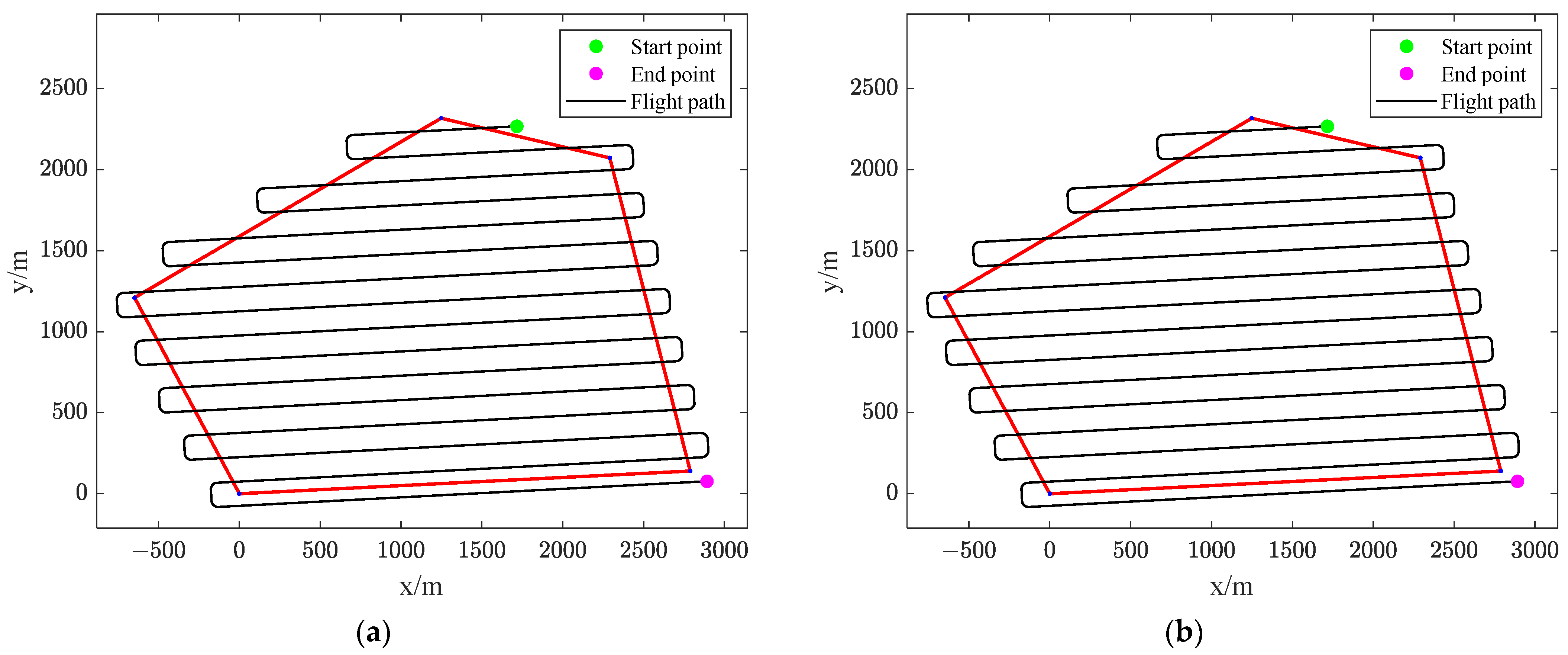
What needs to be pointed out is that when the $R_{\min }$ is much smaller than the width of a sub-region $w$, that is $\lambda =1$, the traditional BF pattern will degenerate to the interlaced BF pattern, as depicted by Remark 1. An example is given to demonstrate this condition as follows.

The flight height, sweep breadth of camera, shooting advance distance, and overlap rate are the same as the first group of simulations. So, the width of a sub-region $w=w_1(1-c)=300\ast (1-0.5)=150$ m. Assuming the UAV is on a slow flight photogrammetry mission, the average speed when flying in straight lines is 13 m/s, the speed of turning is 10 m/s, and the roll angle $\delta$ is 15 degrees. Thus, we have the minimum turning radius $R_{\min }=40$ m according to Equation (5), and the span coefficient $\lambda =1$ by Equation (8). Figure 13a shows the coverage path that is generated by the interlaced BF flight pattern, and the path that is generated by the traditional method is shown in Figure 13b. It can be found that the coverage paths are the same by different methods.

The path parameters of the coverage path generated by different flight patterns when $\lambda =1$ are shown in

Table 5. Path comparison of different flight pattern when $\lambda =1$.

Path Parameters	Interlaced BF Pattern	Traditional BF Pattern	Percentage of Improvement
Number of turns	15	15	0%
The curve path length of turns(m)	1885.1	1885.1	0%
The straight path length of turns(m)	1050.0	1050.0	0%
The total path length of turns(m)	2935.1	2935.1	0%
The total path length(m)	47,996.3	47,996.3	0%
Flight time(s)	3759.8	3759.8	0%

. The presented method performs the same as the conventional method in the condition of $\lambda =1$, and the presented interlaced BF pattern outperforms the traditional BF pattern when $\lambda \ge 2$ according to Result 1, Result 2 and Result 3.

By the above groups of simulation experiments, we can conclude that the proposed interlaced BF pattern is superior to the traditional BF pattern, in terms of the curve path length of turns, the total path length of turns, and the total path length, is more efficient and there is less energy consumption.

6. Conclusions

In this paper, a practical interlacing-based coverage path planning method for a fixed-wing UAV photogrammetry in convex polygon regions was introduced. A typical detection scenario of a camera pointing forward-down for photogrammetry was modeled and the coordinates of the ROI vertices were converted from the WGS-84 coordinate system to the local ENU coordinate system for path planning convenience. The main contribution of this paper is that it fully studies the relationship between the minimum turning radius and the camera footprint. The span coefficient of the fixed-wing UAV was first proposed, and a novel flight pattern, named as the interlaced back-and-forth pattern, was presented accordingly. By comparison with the traditional back-and forth pattern, four results were given and, most importantly, the curve path length of a turn by the interlaced turning strategy was proved to be always shorter than that of the traditional turning strategy in mathematics. In addition, a practical low-computation algorithm for waypoints generation was given. Finally, three groups of simulation experiments that compared the proposed interlaced BF pattern with the traditional BF pattern were conducted. Simulation results showed that the proposed interlaced BF pattern is superior to the traditional BF pattern not only in terms of the path length of turns but also in terms of the total path length.

However, there were some limitations in this work. Firstly, the generated coverage paths in simulations were ideal paths, which did not consider real-world disturbances, such as wind. In future work, we will conduct real-world flight experiments and study wind disturbances. Secondly, only a convex polygon ROI was considered in the presented work. More complex ROIs combined with the interlaced BF flight pattern could be studied in the future. Lastly, it is important to mention that multi-UAV collaboration is a trend; multi-UAV cooperative photogrammetry is left as a future development.