Anti-Interception Guidance for Hypersonic Glide Vehicle: A Deep Reinforcement Learning Approach

Abstract

Anti-interception guidance can enhance a hypersonic glide vehicle (HGV) compard to multiple interceptors. In general, anti-interception guidance for aircraft can be divided into procedural guidance, fly-around guidance and active evading guidance. However, these guidance methods cannot be applied to an HGV’s unknown real-time process due to limited intelligence information or on-board computing abilities. In this paper, an anti-interception guidance approach based on deep reinforcement learning (DRL) is proposed. First, the penetration process is conceptualized as a generalized three-body adversarial optimal (GTAO) problem. The problem is then modelled as a Markov decision process (MDP), and a DRL scheme consisting of an actor-critic architecture is designed to solve this. Reusing the same sample batch during training results in fewer serious estimation errors in the critic network (CN), which provides better gradients to the immature actor network (AN). We propose a new mechanismcalled repetitive batch training (RBT). In addition, the training data and test results confirm that the RBT can improve the traditional DDPG-based-methodes.

1. Introduction

A hypersonic glide vehicle (HGV) has the advantages of a ballistic missile and a lifting body vehicle. It is efficient as it does not require any additional complex anti-interception mechanisms (e.g., carrying a defender to destroy an interceptor [1] or relying on the range advantage of a high-powered onboard radar for early evasion before the interceptor locks on [2]), and can achieve penetration through anti-interception guidance. Over the past decade, studies have focused on utilizing HGV manoeuvreability to protect against interceptors.

In general, anti-interception guidance for aircraft has three categories: (1) procedural guidance [3,4,5,6], (2) fly-around guidance [7,8], and (3) active evading guidance [9,10].

Early research on anti-interception guidance focused on procedural guidance. In procedure guidance, the desired trajectory (such as sine manoeuvres [5], square wave manoeuvres [3], or snake manoeuvres [6]) is planned prior to launch based on facts such as the target position, interceptor capability and manoeuvre strategy, and the vehicle receives guidance based on the fixed trajectory after launch. Imado et al. [11] studied the lateral procedural guidance in a horizontal plane. Zhang et al. [12] proposed a midcourse penetration strategy using an axial impulse manoeuvre and provided a detailed trajectory design method. This penetration strategy does not require lateral pulse motors. To eliminate the re-entry error caused by midcourse manoeuvre, Wu et al. [13] used the remaining pulse motors to regress a preset ballistic. Procedural guidance only needs to plan a ballistic and inject it into the onboard computer before launch, which is easy to implement and does not occupy onboard computing resources. With the advancement of interception guidance, the procedural manoeuvres studied by Imado et al. [11,12] may be recognized by interceptors, and effectiveness cannot be guaranteed when fighting against advanced interceptors.

In conjunction with the advances in planning and information fusion, fly-around the detection zone has emerged as a penetration strategy. The primary objective is to plan a trajectory that can evade an enemy’s detection zone. A complex nonlinear programming problem with multiple constraints and stages is used to achieve this objective. In terms of the detection zone, Zhang et al. [14] established infinitely high cylindrical and semi-ellipsoidal detection zone models under the assumption of earth-flattening and optimized the trajectory that satisfies the waypoint and detection zone constraints. Zhao et al. [7] proposed adjusting the interval density with curvature and error criteria based on the multi-interval pseudo-spectrum method. An adaptive pseudo-spectrum method was constructed to solve the multi-interval pseudo-spectrum, and the number of points in the interval was allocated. A rapid trajectory optimization algorithm was also proposed for the whole course under the condition of multiple constraints and multiple detection zones. However, fly-around guidance has insufficient adaptability on the battlefield. Potential re-entry points have a wide distribution, and the circumvention methods studied by Zhang et al. [7,14], cannot guarantee that a planned trajectory will meet energy constraints. In addition, there may not be a trajectory that can evade all detection zones in an enemy’s key air defence area. Moreover, it may be impossible to know an enemy’s detection zones due to limited intelligence.

As onboard air-detection capabilities have advanced, active evading has gradually gained popularity in anti-interception guidance, and some research results have been recorded through differential game (DG) theory and numerical optimization algorithms in recent years. In DG, Hamilton functions are built based on an adversarial model and are then solved by numerical algorithms to find the optimal control using real-time aircraft flight states. Xian et al. [15] conducted research based on DG and achieved a strategy set of evasion manoeuvres. According to the accurate model of a penetration spacecraft and an interceptor, Bardhan et al. [4] proposed guidance using a state-dependent Riccati equation (SDRE). This approach obtained superior combat effectiveness compared with traditional DG. However, DG requires many calculations and has poor real-time performance. Model errors can be introduced during linearization [16], and onboard computers have difficulty achieving high-frequency corrections. The ADP algorithm was employed by Sun et al. [17,18] address with the horizontal flight pursuit problem. In an attempt to reduce the computational complexity, neural networks were used to fit the Hamilton function online. However, it is unclear whether this idea can be adapted for an HGV featuring a gaint flight envelope. Numerical optimization algorithms, for example, pseudo-spectral methods [19,20] have been used to discretize complex nonlinear HGV differential equations and convert various types of constraints into algebraic constraints. Various optimization methods, such as convex optimization or sequential quadratic programming, are used to solve the optimal trajectory. The main drawback of applying numerical optimization algorithms to HGV anti-interception guidance is that they occupy a considerable amount of onboard computer resources over a long period of time, and the computational time required increases exponentially with the number of aircrafts. Due to these limitations, active evading guidance is unsuitable for engineering.

Reinforcement learning (RL) is a model-free algorithm that is used to solve decision-making problems and has gained attention in the control field because it is entirely based on data, does not require model knowledge, and can perform end-to-end self-learning. Due to the limitations of traditional RL, early research cannot handle high-dimensional and continuous battlefield state information. In recent years, deep neural networks (DNNs) have demonstrated the ability to approximate an arbitrary function and have unparalleled advantages in the feature extraction of high-dimensional data. Deep reinforcement learning (DRL), is a technique resulting from the intersection of DNN and RL, and its abilities can exceed those of human empirical cognition [21]. A wave of research into DRL has been sparked by successful applications, such as Alpha-Zero [22] and Deep Q Networks (DQN) [23,24]. After training, a DNN can quickly output control in milliseconds and has a good generalization ability in unknown environments [25]. Therefore, DRL has promising applications in aircraft guidance. There has been some discussion regarding using DRL to train DNNs in intercepting a penetration aircraft [26]. Brain et al. [27] used reinforcement meta-learning to optimize an adaptive guidance system that is suitable for the approach phase of an HGV. However, no research has been conducted on the application of DRL to HGV anti-interception guidance. However, some studies in different areas have examined similar questions. Wen et al. [28] proposed a collision avoidance method based on a deep deterministic policy gradient (DDPG) approach, and a proper heading angle was obtained by using the proposed algorithm to guarantee conflict-free conditions for all aircraft. For micro-drones flying in orchards, Lin et al. [29] implemented DDPG to create a collision-free path. Guo et al. studied a similar problem, the difference being that DDPG was applied to an unmanned ship. Lin et al. [30] studied how to use DDPG to train a fully connected DNN to avoid collision with four other vehicles by controlling the acceleration of the merging vehicle. For unmanned surface vehicles (USVs), Xu et al. [31] used DDPG to determine the switching time of path-planning and dynamic collision avoidance. These studies led us to believe that DDPG-based methods have promising applications for solving the anti-interception guidance problem of HGVs. However, due to the differences in the objects of study, the anti-interception guidance problem for HGVs requires consideration of some of the following issues: (1) The performance (especially the available overload) of an HGV is time-varying due to the velocity and altitude, while the performance of the control object is fixed in the abovementioned studies. We need to build a model in which the DDPG training process is not affected by time-varying performance. (2) The end state is the only concern in the anti-intercept guidance problem, and only one instant reward is obtained in a training episode. Therefore, sparsity and the delayed reward effect are more significant in this study than in the studies mentioned above. In this paper, we attempt to improve the existing DDPG-based methods to help DNNs gain intelligence faster.

The main contributions of this paper are as follows: (1) Anti-interception HGV guidance is described as an optimization problem, and a generalized three-body adversarial optimization (GTAO) model is developed. This model does not need to account for the severe constraints in the available overload (AO) and is suitable for DRL. To our knowledge, this is the first time that DRL-specific application was implemented for the anti-interception guidance of an HGV. (2) A DRL scheme is developed to solve the GTAO problem, and the RBT-DDPG algorithm is proposed. Compared with the traditional DDPG-based algorithm, the RBT-DDPG algorithm can improve the learning effects of the critic network (CN), alleviate the exploration–utilization paradox, and achieve a better performance. In addition, since the forward computation of a fully connected neural network is very simple, an intelligent network trained by DRL can quickly compute a command for anti-interception guidance that matches the high dynamic characteristics of the HGV. (3) A strategy review of teh HGV anti-interception guidance derived from the DRL approach is provided. We note that this is the first time that these strategies are summarized for HGV guidance through semantics, and may inspire the research community.

The remainder of this paper is organized as follows: Section 2 describes the problem of anti-interception guidance for HGVs as an optimization problem and translates the problem into solving a Markov decision process (MDP). In Section 3, the RBT-DDPG algorithm is given in detail. Moreover, we propose a specific design of the state space, action space, and reward functions that are necessary to solve the MDP using DRL. Section 4 examines the training and test data and the specific anti-interception strategy. Section 5 presents a conclusion to the paper and an outlook on intelligent guidance.

2. Problem Description

Figure 1 shows the path of an HGV conducting an anti-interception manoeuvre. The coordinate and velocity of the aircraft are known, as well as the coordinate of the desired regression point (DRP). The HGV and interceptor rely on aerodynamics to perform ballistic manoeuvres. The aerodynamic forces are mainly derived from the angle of attack (AoA). As an HGV can glide for thousands of kilometres, this paper focuses on the guidance needed after the interceptors locked on the HGV, and the flight distance of this process is set to 200 km.

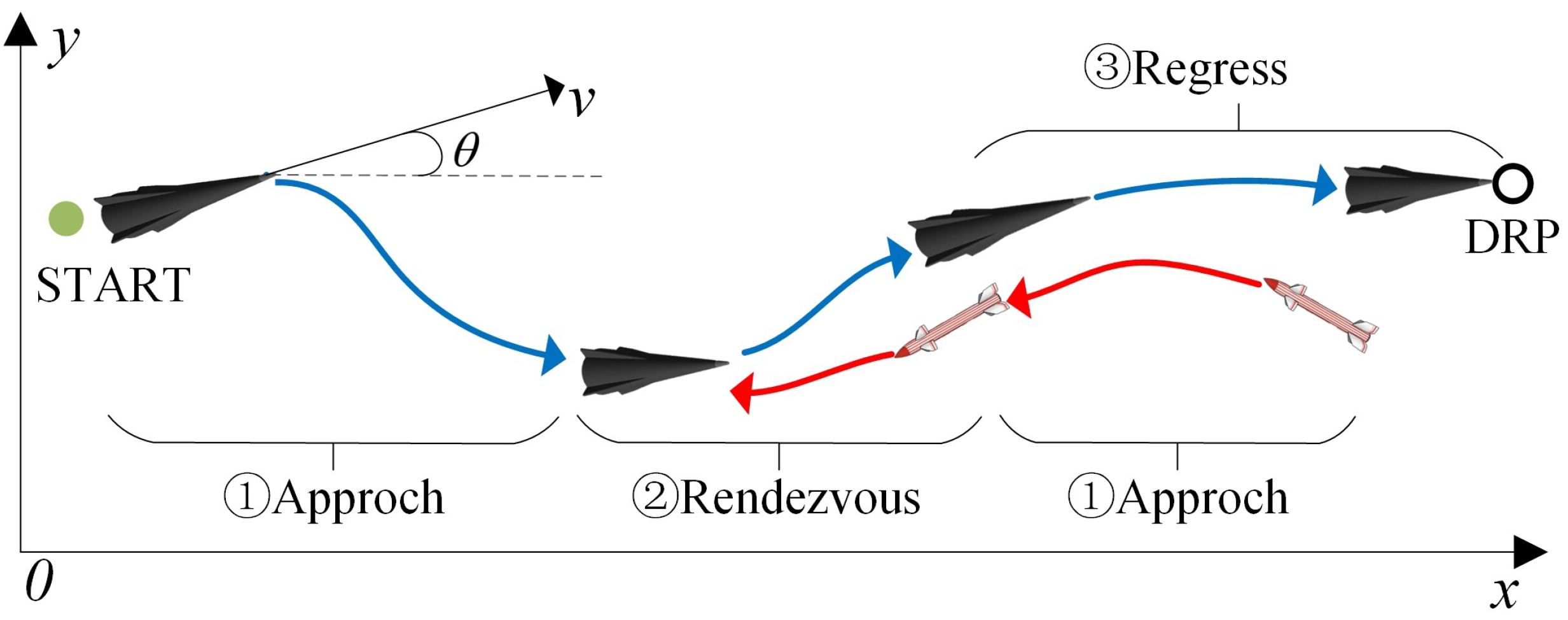
2.1. The Object of Anti-Interception Guidance

In the Earth-centered earth-fixed frame, the motion of the aircraft in the vertical plane is described as follows [32]:

$$\left\{\begin{array}{c}\frac{\mathrm{d}v}{\mathrm{d}t}=\frac{1}{m}\left(Pcos\alpha -C_X\left(v,\alpha \right)qS\right)-gsin\theta \hfill \\ \frac{\mathrm{d}\theta }{\mathrm{d}t}=\frac{1}{mv}\left(Psin\alpha +C_Y\left(v,\alpha \right)qS\right)-\left(\frac{g}{v}-\frac{v}{R_0+y}\right)cos\theta \hfill \\ \frac{\mathrm{d}x}{\mathrm{d}t}=\frac{R_{0}vcos\theta }{R_0+H}\hfill \\ \frac{\mathrm{d}y}{\mathrm{d}t}=vsin\theta \hfill \end{array}\right.$$

(1)

where x is the flight distance, y is the altitude, v is the flight velocity, $\theta$ is the ballistic inclination, g is the gravity acceleration, $R_0$ is the mean radius of the earth when the flatness of the earth is ignored, $C_X\left(v,\alpha \right)$ and $C_Y\left(v,\alpha \right)$ are the lift and drag aerodynamic coefficients of the aircraft, respectively, $\alpha$ is the AoA, q is the dynamic pressure, S is the aerodynamic reference area, m is the mass of the vehicle, and P is the engine thrust.

Letting subscript $\mathrm{H}$ and $\mathrm{I}$ indicate the variables subordinate to the HGV and interceptor, respectively. Setting ${\mathit{x}}_{\mathrm{H}}\left(t\right)={\left[\begin{array}{cccc}x& y& v& \theta \end{array}\right]}^{\mathrm{T}}$ is the state of an axisymmetric HGV, then Equation (1) can be rewritten as follows:

$${\dot{\mathit{x}}}_{\mathrm{H}}\left(t\right)={\mathit{f}}_{\mathrm{H}}\left({\mathit{x}}_{\mathrm{H}}\right)+{\mathit{g}}_{\mathrm{H}}\left({\mathit{x}}_{\mathrm{H}}\right)u\left(t\right)=\left[\begin{array}{c}\frac{R_{0}vcos\theta }{R_0+H}\\ vsin\theta \\ -\frac{C_{X}qS}{m}-gsin\theta \\ -\left(\frac{g}{v}-\frac{v}{R_0+y}\right)cos\theta \end{array}\right]+\left[\begin{array}{c}0\\ 0\\ 0\\ {\delta }_{\mathrm{H}}\left({\mathit{x}}_{\mathrm{H}}\right)\end{array}\right]u\left(t\right)$$

(2)

where ${\delta }_{\mathrm{H}}\left({\mathit{x}}_{\mathrm{H}}\right)=\underset{\alpha }{max}\left(\frac{1}{mv}{C}_Y\left(v,\alpha \right)qS\right)$ is the maximum rate of inclination generated by aerodynamics in state ${\mathit{x}}_{\mathrm{H}}$. The $u\left(t\right)\in \left[\begin{array}{cc}-1,& 1\end{array}\right]$ is the command of the guidance.

Remark 1.

${\delta }_{\mathrm{H}}\left({\mathit{x}}_{\mathrm{H}}\right)$ is related to y, v of the vehicle and the available AoA, so its value varies with ${\mathit{x}}_{\mathrm{H}}\left(t\right)$. The purpose of this procedure is to place $u\left(t\right)$ into a constant range, ensuring that the manoeuvring ability required for guidance always follows the real-time AO under the giant flight envelope of the HGV.

Remark 2.

The reason for using $u\left(t\right)$ as the control variable, instead of directly using the AoA α, is that it is possible to rely on an existing model to calculate ${\delta }_{\mathrm{H}}\left({\mathit{x}}_{\mathrm{H}}\right)$ and input it into the neural network (as shown in Section 3), thus omitting the neural network training process in the maximum available overload.

As the long-range interceptor is in the target-lock state, its booster rocket is switched off and unpowered with state ${\mathit{x}}_{\mathrm{I}}\left(t\right)={\left[\begin{array}{cccc}x& y& v& \theta \end{array}\right]}^{\mathrm{T}}$. The motion is as follows:

$${\dot{\mathit{x}}}_{\mathrm{I}}\left(t\right)=f_{\mathrm{I}}\left({\mathit{x}}_{\mathrm{I}},{\mathit{x}}_{\mathrm{H}}\right)=\left[\begin{array}{c}\frac{R_{0}vcos\theta }{R_0+H}\\ vsin\theta \\ -\frac{C_{X}qS}{m}-gsin\theta \\ G_{\mathrm{I}}\left({\mathit{x}}_{\mathrm{I}},{\mathit{x}}_{\mathrm{H}},t\right)\end{array}\right]$$

(3)

where $G_{\mathrm{I}}\left({\mathit{x}}_{\mathrm{I}},{\mathit{x}}_{\mathrm{H}},t\right)$ is the actual rate of inclination under the influence of the guidance and control system.

Remark 3.

As the focus of this paper is on the centre-of-mass motion of vehicles, it is assumed that the vehicles always follow the guidance under the effects of the attitude control system, so errors in attitude control are ignored in Equations (2) and (3), as well as minor effects such as Gauche forces and implicated accelerations.

HGV and N interceptors can form a nonlinear system:

$${\dot{\mathit{x}}}_{\mathrm{S}}\left(t\right)={\mathit{f}}_{\mathrm{S}}\left({\mathit{x}}_{\mathrm{S}}\right)+{\mathit{g}}_{\mathrm{S}}\left({\mathit{x}}_{\mathrm{S}}\right)u\left(t\right)$$

(4)

where system state is ${\mathit{x}}_{\mathrm{S}}={\left[\begin{array}{cc}{\left({\mathit{x}}_{\mathrm{H}}\right)}^{\mathrm{T}}& {\left({\mathit{x}}_{\mathrm{I}1}\right)}^{\mathrm{T}}\begin{array}{cc}\dots & {\left({\mathit{x}}_{\mathrm{I}N}\right)}^{\mathrm{T}}\end{array}\end{array}\right]}^{\mathrm{T}}$, the nonlinear kinematics of the system are $f_{\mathrm{S}}\left({\mathit{x}}_{\mathrm{S}}\right)={\left[\begin{array}{cc}\left(f_{\mathrm{H}}\right)& \left(f_{\mathrm{I}1}\right)\begin{array}{cc}\dots & \left(f_{\mathrm{I}N}\right)\end{array}\end{array}\right]}^{\mathrm{T}}$ and the non-linear effect of control is $g_{\mathrm{S}}\left({\mathit{x}}_{\mathrm{S}}\right)={\left[\begin{array}{cc}{\left(g_{\mathrm{H}}\right)}^{\mathrm{T}}& O_{{}^{1\times 4N}}\end{array}\right]}^{\mathrm{T}}$.

The guidance system aims to control the system described in Equation (4) using $u\left(t\right)$ to achieve penetration. Therefore, the design of an anti-interception guidance can be viewed as an optimal control problem. First, the HGV must successfully evade the interceptor during penetration, and then reach the DRP ${\mathit{P}}_{\mathrm{E}}={\left[\begin{array}{cc}{\mathit{x}}_{\mathrm{E}}& y_{\mathrm{E}}\end{array}\right]}^{\mathrm{T}}$ to conduct the follow-up mission. Let $t_{\mathrm{f}}$ be the time that the HGV arrives at ${\mathit{x}}_{\mathrm{E}}$, and let $u\left(t\right)$ direct system Equation (4) to state ${\mathit{x}}_{\mathrm{S}}\left(t_{\mathrm{f}}\right)$. The anti-interception guidance is designed to solve the following GTAO problem [33].

As mentioned in Equation (4), an HGV and its opponents form a system represented by ${\mathit{x}}_{\mathrm{S}}$. The initial value of ${\mathit{x}}_{\mathrm{S}}$ is:

$${\mathit{x}}_{\mathrm{S}}\left(t_0\right)={\left[\begin{array}{cccccccc}{\mathit{x}}_{\mathrm{H},0}& y_{\mathrm{H},0}& v_{\mathrm{H},0}& {\theta }_{\mathrm{H},0}& \dots {\mathit{x}}_{\mathrm{I}N,0}& y_{\mathrm{I}N,0}& v_{\mathrm{I}N,0}& {\theta }_{\mathrm{I}N,0}\end{array}\right]}^{\mathrm{T}}$$

(5)

The process constraint of penetration:

$$min\left({\left({\mathit{M}}_{x,i}{\mathit{x}}_{\mathrm{S}}\left(t\right)\right)}^2+{\left({\mathit{M}}_{y,i}{\mathit{x}}_{\mathrm{S}}\left(t\right)\right)}^2\right)>R^2,i\in \left[1,N\right]$$

(6)

where ${\mathit{M}}_{x,i}=\left[\begin{array}{cccc}1& {\mathit{O}}_{{}^{1\times 3}}& {\mathit{O}}_{{}^{1\times 4(i-1)}}& \begin{array}{cc}-1& \begin{array}{cc}{\mathit{O}}_{{}^{1\times 3}}& {\mathit{O}}_{{}^{1\times 4(N-i)}}\end{array}\end{array}\end{array}\right]$, and R is the kill radius of the interceptor, ${\mathit{M}}_{y,i}=\left[0\hspace{1em}1\hspace{1em}{\mathit{O}}_{1\times 2}\hspace{1em}{\mathit{O}}_{1\times 4(i-1)}\hspace{1em}0\hspace{1em}-1\hspace{1em}{\mathit{O}}_{1\times 2}\hspace{1em}{\mathit{O}}_{1\times 4(N-i)} \right]$.

The process constraint of heat flux is:

$${\left(q_{\mathrm{S}}\right)}_{3\mathrm{D}}\le q_{\mathrm{U}}$$

(7)

where ${\left(q_{\mathrm{S}}\right)}_{3\mathrm{D}}$ is the three-dimensional stagnation point of the heat flux and $q_{\mathrm{U}}$ is the upper limit of the heat flux. For an arbitrarily shaped, three-dimensional stagnation point with a radius of curvature $R_1$ and $R_2$, the heat flux is expressed as:

$${\left(q_{\mathrm{S}}\right)}_{3\mathrm{D}}=\sqrt{\frac{1+k}{2}}{\left(q_{\mathrm{S}}\right)}_{\mathrm{AXI}}$$

(8)

where $k=\frac{R_1}{R_2}$ and ${\left(q_{\mathrm{S}}\right)}_{\mathrm{AXI}}$ is the axisymmetric heat flux, which is related to the flight altitude and velocity [34].

The minimum velocity constraint:

$$\left[\begin{array}{ccc}{\mathit{O}}_{{}^{1\times 2}}& 1& \begin{array}{cc}0& {\mathit{O}}_{{}^{1\times 4}}\end{array}\end{array}\right]{\mathit{x}}_{\mathrm{S}}\ge V_{min}$$

(9)

The control constraint:

$$u\left(t\right)\in \left[\begin{array}{cc}-1& 1\end{array}\right]$$

(10)

The objective function is a Mayer type function:

$$J\left({\mathit{x}}_{\mathrm{S}}\left(t_0\right),u\left(t\right)\right)=Q\left({\mathit{x}}_{\mathrm{S}}\left(t_f\right)\right)$$

(11)

where $Q\left({\mathit{x}}_{\mathrm{S}}\left(t_f\right)\right)={\left({\mathit{x}}_{\mathrm{S}}\left(t_f\right)-{\tilde{\mathit{P}}}_{\mathrm{E}}\right)}^{\mathrm{T}}\mathit{R}\left({\mathit{x}}_{\mathrm{S}}\left(t_f\right)-{\tilde{\mathit{P}}}_{\mathrm{E}}\right)$, ${\tilde{\mathit{P}}}_{\mathrm{E}}={\left[\begin{array}{cc}{{\mathit{P}}_{\mathrm{E}}}^{\mathrm{T}}& \begin{array}{cc}{V}_{min}& {\mathit{O}}_{{}^{1\times \left(4N+1\right)}}\end{array}\end{array}\right]}^{\mathrm{T}}$ and $\mathit{R}=\left[\begin{array}{cccc}0& & & \\ & -w_1& & \\ & & w_2& \\ & & & {\mathit{O}}_{{}^{(4N+1)\times (4N+1)}}\end{array}\right]$ in which $w_1$, $w_2\in \mathbb{R}{}^{+}$ are weights.

The optimal performance:

$$J^{*}\left({\mathit{x}}_{\mathrm{S}}\left(t_0\right)\right)=\underset{u\left(t\right),t\in \left[t_0,t_{\mathrm{f}}\right]}{max}J\left({\mathit{x}}_{\mathrm{S}}\left(t_0\right),u\left(t\right)\right)$$

(12)

From Equation (12), the optimal control $u^{*}\left(t\right)$ is determined by ${\mathit{x}}_{\mathrm{S}}\left(t_0\right)$. After obtaining all the model information of system Equation (4), the optimal state trajectory of the system can be found according to ${\mathit{x}}_{\mathrm{S}}\left(t_0\right)$ using static optimization methods (e.g., quadratic programming). Nevertheless, resolving the problem using optimization methods is challenging, especially since there is limited information about the interceptor (aerodynamic parameters, available overload, guidance, etc.).

2.2. Markov Decision Process

The MDP can model a sequential decision problem and is well-suited to the HGV anti-interception process. The MDP can be defined by a five-tuple $〈\mathcal{S},\mathcal{A},T,R,\gamma 〉$ [35]. $\mathcal{S}$ is a multidimensional continuous state space. $\mathcal{A}$ is an available action space. T is a state transition function: $\mathcal{S}\times \mathcal{A}\to \mathcal{S}$. That is, after an action $a\in \mathcal{A}$ is taken in the state $\mathit{s}\in \mathcal{S}$, the state changes from s to ${\mathit{s}}^{\prime }\in \mathcal{S}$. R is an instant reward function: it represents an instant reward obtained from the state transition. $\gamma \in [0,1]$ is a constant discount factor used to balance the importance of the instant reward and forward reward.

The cumulative reward obtained by the controller under the command sequence $\tau =\{a_0,\dots ,a_n\}$ is:

$$G({\mathit{s}}_0,\tau )=\sum _{t=0}^{\infty }{\gamma }^t{r}_t$$

(13)

The expected value function of the cumulative reward based on state ${\mathit{s}}_t$ and the expected value function of $({\mathit{s}}_t,a_t)$ are introduced as shown below:

$$V^{\pi }\left({\mathit{s}}_t\right)=\mathbb{E}\left[\sum _{k=0}^{\infty }{\gamma }^k{r}_{t+k}|{\mathit{s}}_t,\pi \right]$$

(14)

$$Q^{\pi }({\mathit{s}}_t,a_t)=\mathbb{E}\left[\sum _{k=0}^{\infty }{\gamma }^k{r}_{t+k}|{\mathit{s}}_t,a_t,\pi \right]$$

(15)

where $V^{\pi }\left({\mathit{s}}_t\right)$ indicates the expected cumulative reward that controller $\pi$ can obtain in the current state ${\mathit{s}}_t$. $Q^{\pi }({\mathit{s}}_t,a_t)$ indicates the expected cumulative reward under controller $\pi$ after executing $a_t$ in state ${\mathit{s}}_t$.

According to the Bellman Optimal theorem [35], updating $\pi \left({\mathit{s}}_t\right)$ through the iteration rule shown in the following equation can be used to approximate the maximum $V^{\pi }\left({\mathit{s}}_t\right)$ value:

$$\pi \left({\mathit{s}}_t\right)=arg\underset{a_t}{max}{Q}^{\pi }({\mathit{s}}_t,a_t)$$

(16)

3. Proposed Method

Section 2 converts the anti-interception guidance of an HGV to an MDP. The key to obtaining optimal guidance is the accurate estimation of $Q^{\pi }({\mathit{s}}_t,a_t)$. Much progress has been made towards artificial intelligence using supervised learning systems trained to replicate human expert decisions. However, expert data are often expensive, unreliable, or unavailable [36], although DRL can still realize accurate $Q^{\pi }({\mathit{s}}_t,a_t)$ estimation. The guidance system needs to process as much data as possible and then choose the next action. The input space of the guidance system has high dimensionality and continuous characteristics, and its action space has continuous characteristics. The DDPG-based methods (the main methods are DDPG and TD3) have been shown to effectively handle high-dimensional continuous information and output continuous actions. They could be used to solve the MDP proposed in this paper. This section aims to achieve faster policy convergence and better performance by optimizing DDPG-based method training. Since the TD3 algorithm has only one more CN pair compared to DDPG, this paper takes RBT-DDPG as an example to introduce how the RBT mechanism improves the training of the critic part. RBT-TD3 is easily obtained by simply repeating the improvements made by RBT-DDPG in each pair of TD3 critic networks.

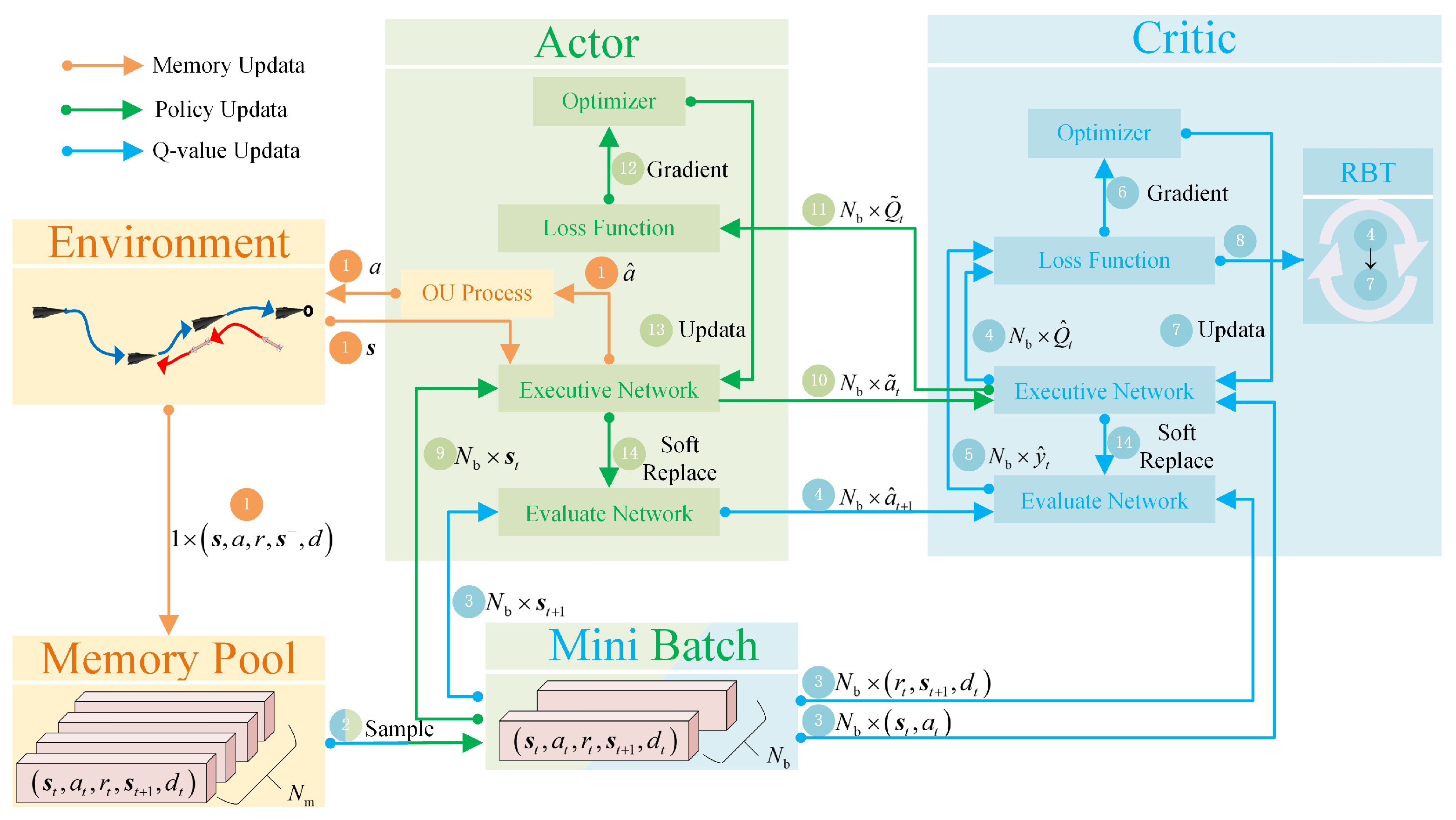
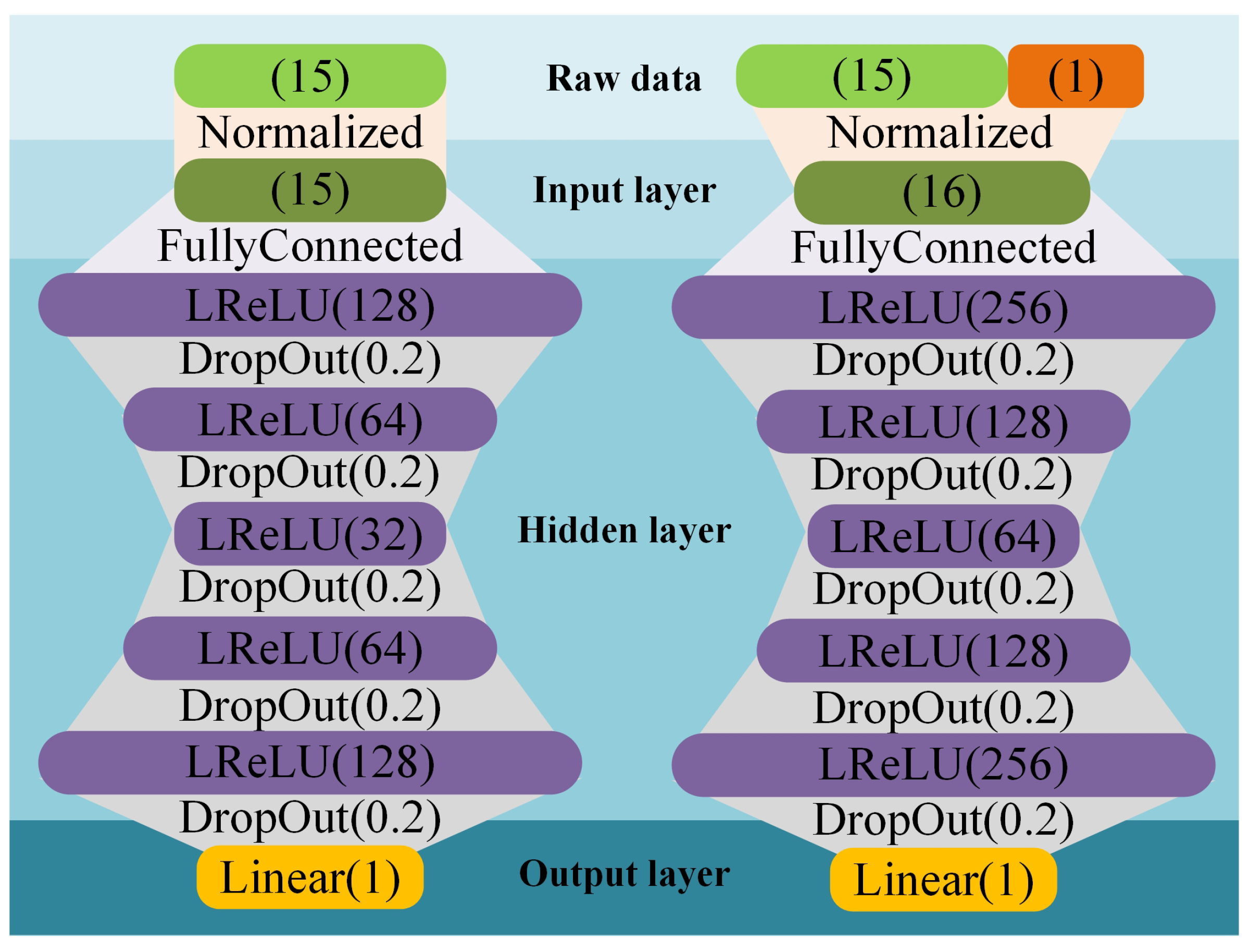
3.1. RBT-DDPG-Based Methods

CN $Q\left(·\right)$ in the DDPG-based methods is only used, during reinforcement learning, to train AN $A\left(·\right)$. At execution, the real action is determined directly by $A\left(·\right)$.

For CN, the DDPG-based optimization objective is to minimize the loss function $L_Q\left({\mathit{\varphi }}_Q\right)$. Its gradient is

$${\nabla }_{{\mathbf{\varphi }}_Q}{L}_Q\left({\mathbf{\varphi }}_Q\right)=\left(\frac{1}{N_b}\sum _{j=1}^{N_b}\left({\nabla }_{{\mathbf{\varphi }}_Q}Q({\mathit{s}}_{t,j},a_{t,j}|{\mathbf{\varphi }}_Q)\right)\right)\left(\frac{2}{N_b}\sum _{j=1}^{N_b}\left(Q({\mathit{s}}_{t,j},a_{t,j}|{\mathbf{\varphi }}_Q)\right)-{\widehat{y}}_t\right)$$

(17)

After a single gradient descent operation is performed, the gradient descent method is only guaranteed to update the parameters in the right direction. The amplitude of the loss function is not guaranteed after a single gradient descent procedure.

For AN, the DDPG-based optimization objective is to minimize the loss function $L_A\left({\mathbf{\varphi }}_A\right)$. Its gradient is

$${\nabla }_{{\mathbf{\varphi }}_A}{L}_{\mathrm{A}}\left({\mathbf{\varphi }}_A\right)=-\frac{1}{N_b}\sum _{j=1}^{N_b}\left({\nabla }_{{\tilde{a}}_{t,j}}Q\left({\mathit{s}}_{t,j},{\tilde{a}}_{t,j}|{\mathbf{\varphi }}_Q\right){\nabla }_{{\mathbf{\varphi }}_A}A\left({\mathit{s}}_{t,j}\right|{\mathbf{\varphi }}_A)\right)$$

(18)

The direction of parameter iteration of AN is affected by CN. The single gradient descent method used by the DDPG-based method does not guarantee accurate CN estimation. In some instances where the estimation is grossly inaccurate, incorrect parameter updates will be provided to AN, further deteriorating the sample data in the memory pool and affecting the training efficiency.

Rather than allowing CN to steer AN in the wrong direction, this paper proposes a new, improved, DDPG-based mechanism: repetitive batch training (RBT). The core idea of RBT, which mainly aims to improve the updating strategy of $Q^{\pi }\left({\mathit{s}}_t,a_t\right)$, is that when a sample batch is used to update the CN parameters, the CN is repetitively trained using the loss function as its reference threshold (as in Equation (19)), thereby avoiding a serious misestimate of CN. The reference threshold $L_{\mathrm{TH}}$ for repeats should be set appropriately.

$$\left\{\begin{array}{c}Repeat,L_Q\left({\mathbf{\varphi }}_Q\right)\ge L_{\mathrm{TH}}\hfill \\ Pass,L_Q\left({\mathbf{\varphi }}_Q\right)<L_{\mathrm{TH}}\hfill \end{array}\right.$$

(19)

$Q\left({\mathit{s}}_{t,j},{\tilde{a}}_{t,j}|{\mathbf{\varphi }}_Q\right)$ is split into two parts:

$$Q\left({\mathit{s}}_{t,j},a_{t,j}|{\mathbf{\varphi }}_Q\right)=Q^{*}\left({\mathit{s}}_{t,j},a_{t,j}|{\mathbf{\varphi }}_{Q^{*}}\right)+D\left({\mathit{s}}_{t,j},a_{t,j}|{\mathbf{\varphi }}_Q\right)$$

(20)

where, $Q^{*}\left({\mathit{s}}_{t,j},a_{t,j}|{\mathbf{\varphi }}_{Q^{*}}\right)$ is the real mapping of Q and $D\left({\mathit{s}}_{t,j},a_{t,j}|{\mathbf{\varphi }}_Q\right)$ is the estimation error. Therefore, Equation (18) is rewritten as:

$${\nabla }_{{\mathbf{\varphi }}_A}{L}_{\mathrm{A}}\left({\mathbf{\varphi }}_A\right)=-\frac{1}{N_b}\sum _{j=1}^{N_b}\left(\left({\nabla }_{{\tilde{a}}_{t,j}}{Q}^{*}\left({\mathit{s}}_{t,j},{\tilde{a}}_{t,j}|{\mathbf{\varphi }}_{Q^{*}}\right)+{\nabla }_{{\tilde{a}}_{t,j}}D\left({\mathit{s}}_{t,j},{\tilde{a}}_{t,j}|{\mathbf{\varphi }}_Q\right)\right){\nabla }_{{\mathbf{\varphi }}_A}A\left({\mathit{s}}_{t,j}\right|{\mathbf{\varphi }}_A)\right)$$

(21)

According to the Taylor expansion:

$${\nabla }_{{\tilde{a}}_{t,j}}D\left({\mathit{s}}_{t,j},{\tilde{a}}_{t,j}|{\mathbf{\varphi }}_Q\right)=\frac{1}{\Delta \tilde{a}}\left(D\left({\mathit{s}}_{t,j},{\tilde{a}}_{t,j}+\Delta \tilde{a}|{\mathbf{\varphi }}_Q\right)-D\left({\mathit{s}}_{t,j},{\tilde{a}}_{t,j}|{\mathbf{\varphi }}_Q\right)-R_2\right)$$

(22)

where $R_2$ is the higher-order residual term. Since $∥D\left({\mathit{s}}_{t,j},{\tilde{a}}_{t,j}|{\mathbf{\varphi }}_Q\right)∥\in \left(0,L_{\mathrm{TH}}\right)$,:

$$∥D\left({\mathit{s}}_{t,j},{\tilde{a}}_{t,j}+\Delta \tilde{a}|{\mathbf{\varphi }}_Q\right)-D\left({\mathit{s}}_{t,j},{\tilde{a}}_{t,j}|{\mathbf{\varphi }}_Q\right)∥<2L_{\mathrm{TH}}$$

(23)

$$∥{\nabla }_{{\tilde{a}}_{t,j}}D\left({\mathit{s}}_{t,j},{\tilde{a}}_{t,j}|{\mathbf{\varphi }}_Q\right)∥<\frac{2L_{\mathrm{TH}}}{∥\Delta \tilde{a}∥}-2∥\frac{R_2}{\Delta \tilde{a}}∥$$

(24)

Naturally, setting $L_{\mathrm{TH}}$ as a small value will reduce the misdirection from the unconverged CN to the AN.

If $L_{\mathrm{TH}}$ is too large, the RBT-DDPG will be weakened. CN will overfit the samples in a single batch if $L_{\mathrm{TH}}$ is too small. The RBT-DDPG shown in Figure 2 and Algorithm 1 is an example of how RBT can be combined with DDPG-based methods.

Algorithm 1 RBT-DDPG

1: Initialize parameters ${\mathbf{\varphi }}_A$,${\mathbf{\varphi }}_{A^{-}}$,${\mathbf{\varphi }}_Q$,${\mathbf{\varphi }}_{Q^{-}}$. 2: for each iteration do 3:     for each environment step do 4:         $a=\left(1-e^{-\theta t}\right)\mu +e^{-\theta t}\widehat{a}+\sigma \sqrt{\frac{1-e^{-2\theta t}}{2\theta }}\epsilon$,$\epsilon \sim \left(0,1\right)$,$\widehat{a}=A\left(s\right)$. 5:     end for 6:     for each gradient step do 7:         Randomly sample $N_{\mathrm{b}}$ samples. 8:         ${\mathbf{\varphi }}_Q\leftarrow {\mathbf{\varphi }}_Q+{\alpha }_{\mathrm{C}}{\nabla }_{{\mathbf{\varphi }}_Q}{L}_Q\left({\mathbf{\varphi }}_Q\right)$. 9:         if $L_{\mathrm{C}}$ >$L_{\mathrm{TH}}$ then 10:            Back to step 7. 11:         end if 12:         ${\mathbf{\varphi }}_A\leftarrow {\mathbf{\varphi }}_A+{\alpha }_{\mathrm{A}}{\nabla }_{{\mathbf{\varphi }}_A}{L}_{\mathrm{A}}\left({\mathbf{\varphi }}_A\right)$. 13:         ${\mathbf{\varphi }}_{Q^{-}}\leftarrow \left(1-s_r\right){\mathbf{\varphi }}_{Q^{-}}+s_r{\mathbf{\varphi }}_Q$. 14:         ${\mathbf{\varphi }}_{A^{-}}\leftarrow \left(1-s_r\right){\mathbf{\varphi }}_{A^{-}}+s_r{\mathbf{\varphi }}_A$. 15:     end for 16: end for

3.2. Scheme of DRL

To approximate $Q^{\pi }\left({\mathit{s}}_t,a_t\right)$ and optimal AN through DRL, the state space, action space and instant reward function are designed as follows.

3.2.1. State Space

As mentioned in Section 2.1, in the vertical plane, the HGV and interceptors follow Equations (2) or (3), and both can be expressed in terms of two-dimensional coordinates: the velocity, and the ballistic inclination. Therefore, the network can predict the future flight state based on the current state. The AN state space is ${\mathcal{S}}_{\mathrm{HI}}={\mathcal{S}}_{\mathrm{H}}\times {\mathcal{S}}_{\mathrm{I}1}\times \dots \times {\mathcal{S}}_{\mathrm{I}N}$, where ${\mathcal{S}}_{\mathrm{H}}\in \mathbb{R}{}^4$ and ${\mathcal{S}}_{\mathrm{I}i}\in \mathbb{R}{}^4$ are the state space of the HGV and the interceptor i, respectively. AN needs to know the AO of the current state ${\mathcal{S}}_{\mathsf{\Omega }}\in \mathbb{R}$ to evaluate the available manoeuvrability. It also needs to know the position of the DRP ${\mathcal{S}}_{\mathrm{D}}\in \mathbb{R}$${}^2$. As a result, the state space of AN is designed as a $7+4N$-dimensional space $\mathcal{S}={\mathcal{S}}_{\mathrm{HI}}\times {\mathcal{S}}_{\Omega }\times {\mathcal{S}}_{\mathrm{D}}$, and the form of each element is $\left({\mathit{x}}_{\mathrm{H}},y_{\mathrm{H}},v_{\mathrm{H}},{\theta }_{\mathrm{H}},{\mathit{x}}_{\mathrm{I}1},y_{\mathrm{I}1},v_{\mathrm{I}1},{\theta }_{\mathrm{I}1},\dots ,{\mathit{x}}_{\mathrm{I}N},y_{\mathrm{I}N},v_{\mathrm{I}N},{\theta }_{\mathrm{I}N},{\omega }_{max},{\mathit{x}}_{\mathrm{D}},y_{\mathrm{D}}\right)$. For CN, an additional action bit is needed, so its input space is $8+4N$-dimensional.

Remark 4.

The definition of the state space used in this paper means that there is a vast input space for the neural network when an HGV is confronted with many interceptors, resulting in many duplicate elements and complicating the training process. An attention mechanism can alleviate this issue by extracting features from the original input space [37]. Typically, two interceptors are used to intercept one target in air defence operations [38]. Therefore, there is only one HGV and two interceptors in the virtual scenario, limiting the input space of the neural networks.

3.2.2. Action Space

As described in Equation (2), since $u\left(t\right)$ is limited to the interval $\left[-1,1\right]$, the output or action of the neural network can easily be defined as $u\left(t\right)$. $u\left(t\right)$ is multiplied by the AO derived from the model information and then applied to the HGV’s flight control system to ensure that the guidance signal meets the dynamical constraints of the current flight state. The neural network only needs to pick a real number within $\left[-1,1\right]$, which indicates the choice of $\dot{\theta }$ as a guidance command subject to AO constraints. From a training perspective, when aiming to bypass the learning process of the AO, it is more straightforward to use the model information directly, rather than adopting the AoA as the action space.

3.2.3. Instant Reward Function

As an essential part of the trial-and-error approach, the instant reward function, guides the networks to learn the optimal strategy. Diverse instant reward functions indicate different behaviour tendencies. The instant reward function affects the quality of the strategy learned by DRL. As in Equation (12), an instant reward function should be designed, with two aims: (1) to determine the distance between the HGV and DRP reward function $r_{\mathrm{E}}\left(·\right)$ at the terminal time $t_f$, and (2) to apply the velocity reward function $r_{\mathrm{D}}\left(·\right)$ at $t_f$. The instant reward function is designed as follows:

$$r\left({\mathit{x}}_{\mathrm{S}}\left(t\right)\right)=\left\{\begin{array}{c}{r}_{\mathrm{E}}\left({\mathit{x}}_{\mathrm{S}}\left(t\right)\right)+r_{\mathrm{D}}\left({\mathit{x}}_{\mathrm{S}}\left(t\right)\right),t=t_f\hfill \\ 0,t<t_f\hfill \end{array}\right.$$

(25)

It is necessary to convert $w_1$ in Equation (11) to a function with a positive domain in order to encourage the HGV to evade interceptors and reach ${\mathit{x}}_{\mathrm{E}}$ during DRL:

$$f\left(x\right)=\frac{1}{w_1+\sqrt{x}}$$

(26)

Remark 5.

If the flight state of the HGV does not meet the various constraints mentioned in Section 2, then the episode ends early, and the instant reward for the whole episode is 0, which introduces the common sparse reward problem in reinforcement learning. However, it is evident from Section 4 that RBT-DDPG-based methods can generate intelligence from sparse rewards.

Remark 6.

An intensive instant reward function similar to that designed by Jiang et al. [39] is not used, since there is no experience to draw on for the HGV anti-interception problem. Furthermore, rather than a Bolza problem, this instant reward function is fully equivalent to the optimization goal, that is, the mayer type problem defined in Equation (12). Moreover, the neural network is not influenced by the human tendencies of strategy exploration, resulting in an in-depth exploration of all strategic options that could approach the global optimum.

Remark 7.

A curriculum-based approach similar to that discussed by Li et al. [40] was attempted, where HGVs can quickly learn to reduce interceptors’ energy using snake manoeuvres. As the policy is solidified at the approach phase, it is difficult to achieve global optimality using this framework, and the obtained performance is significantly lower than that obtained by Equation (25).

4. Training and Testing

Section 3 introduces RBT-DDPG-based methods to solve the GTAO problem discussed in Section 2. This section verifies the effectiveness of DRL in finding the optimal anti-interception guidance system.

4.1. Settings

4.1.1. Aircraft Settings

To simulate a random initial interceptor energy state in a virtual scenario, the interceptors’ initial altitude and initial velocity follow a uniform distribution and are $U\left(25\mathrm{km},45\mathrm{km}\right)$ and $U\left(1050\mathrm{m}/\mathrm{s},1650\mathrm{m}/\mathrm{s}\right)$ respectively.

Table 1. Parameters of theHGV and interceptor in the virtual scenario.

Parameter	Interceptor	HGV
Mass/kg	75	500
Reference area/m${}^2$	0.3	0.579
Minimum velocity/(m/s)	400	1000
Available AoA/°	−20∼20	−10∼10
Time constant of Attitude Control System/s	0.1	1
Initial coordinate x/km	200	0
Initial coordinate y/km	Random	35
Initial velocity/(km/s)	Random	2000
Initial inclination/°	0	0
Coordinate x of the DRP/km	-	200
Coordinate y of the DRP/km	-	35
Kill radius/m	300	-

illustrates the remaining parameters.

The aerodynamics of an aircraft are usually approximated by the curve-fitted model (CFM). The CFM of the HGV used in this paper is referenced in Wang et al. [41]: $C_{\mathrm{L}}=-0.21+0.075·M+\left(0.23+0.05·M\right)·\alpha$ and $C_{\mathrm{D}}=0.41+0.011·M+\left(-0.0081+0.0021·M\right)·\alpha +0.0042·{\alpha }^2$. M is the Mach number of the HGV and $\alpha$ is the AoA (rad). Morever, the interceptors are $C_{\mathrm{L}}=\left(0.18+0.02·M\right)·\alpha$ and $C_{\mathrm{D}}=0.18+0.01·M+0.001·M·\alpha +0.004·{\alpha }^2$ [42]. The interceptors employ a proportional guide. To compensate for the lack of representation of the vectoring capability in the virtual scenario, we increased the interceptors’ kill radius to a staggering 300 m.

4.1.2. Hyperparameter Settings

Hyperparameters of training are shown in

Table 2. Hyperparameters of RBT-DDPG and RBT-TD3.

Parameter	Value
$\Delta t$/s	${10}^{-2}$
$T_{\mathrm{c}}$/s	1
$\gamma$	1
${\alpha }_{\mathrm{C}}$	${10}^{-4}$
${\alpha }_{\mathrm{A}}$ in RBT-DDPG	${10}^{-4}$
${\alpha }_{\mathrm{A}}$ in RBT-TD3	$5\times {10}^{-5}$
$s_r$	$0.001$
$\mu$ in RBT-DDPG	$0.05$
$\sigma$ in RBT-DDPG	$0.01$
$\theta$ in RBT-DDPG	$5\times {10}^{-5}$
$\sigma$ in RBT-TD3	$0.1$
$L_{\mathrm{TH}}$	$0.1$
Weight initialization	$N(0,0.02)$
Bias initialization	$N(0,0.02)$
$w_1$	$0.5$
$w_2$	${10}^{-4}$

.

In AN, it is evident that the bulk of computation occurs in the hidden layer. A neuron in the hidden layer reads in $n_i$ ($n_i$ is the width of the previous layer) numbers according to a dropOut layer( the drop rate is 0.2), multiplies them by the weight (totalling $2n_i+0.8n_i$ FLOPs), adds up all the values (totalling $n_i$ FLOPs), then passes the result through the activation function (LReLU) after adding a bias term (totaling 2 FLOPs), which means that a single neuron consumes $3.8n_i+3$ FLOPs in a single calculation. The actor, as shown in Figure 3, consumes approximately 87K FLOPs in a single execution. Assuming an on-board computer with ${10}^{-3}$ FLOP floating-point capabilities (most mainstream industrial FPGAs in 2021 have more than a 1 FLOP floating-point capability), a single execution of anti-interception guidance formed by AN takes less than 0.1 ms.

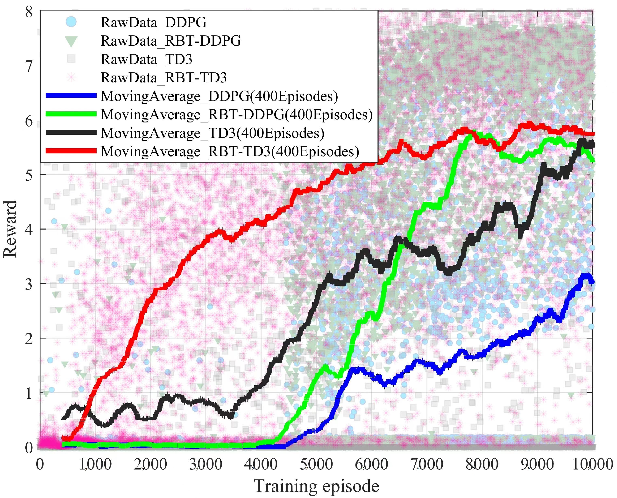
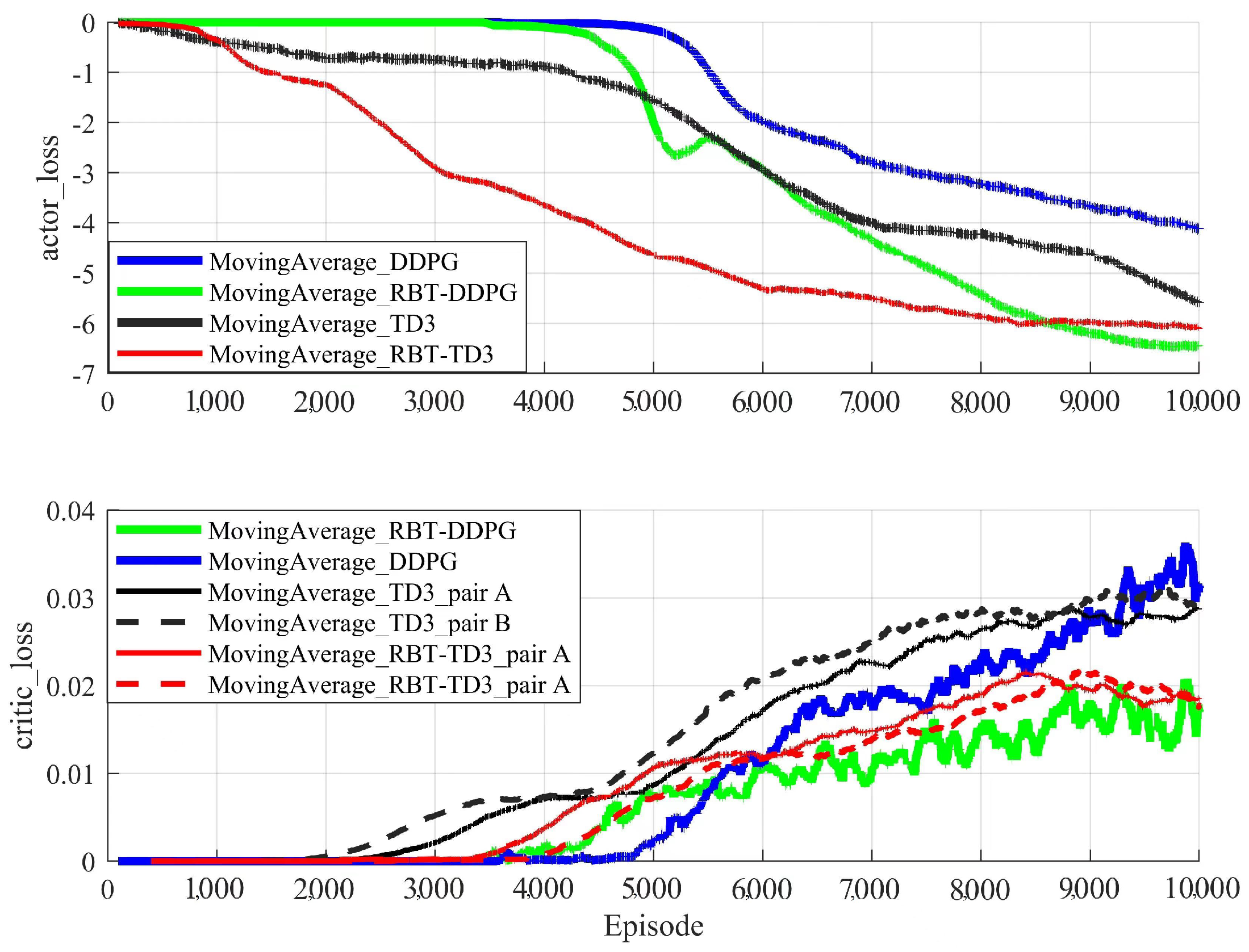
4.2. Training Results and Analysis

The CPU of the training platform is an AMD Ryzen5 [email protected] GHz. The RAM is 8 GB × 2 DDR4@3733 MHz. As the networks are straightforward and the computation is concentrated on calculating aircraft models, GPUs are not selected for training. The aircraft models in the virtual scenario are written in C++ and packaged as a dynamic link library (DLL). The networks and training algorithm are implemented by Python. The networks and the virtual scenario interact after calling the DLL. The training process is shown in Figure 4, Figure 5 and Figure 6.

For episodes 0–3500, DDPG and RBT-DDPG are in the process of constructing their memory pool. The neural networks approximate a random output in this process, and no training occurs. As a result, cumulative rewards are near 0 for most episodes, with a slim possibility of reaching six points through random exploration. The neural networks begin to be iteratively updated as soon as the memory pool is complete. The RBT-DDPG exceeds the maximum score of the random exploration process at approximately 3900 episodes, which is close to seven points. The RBT-DDPG then gradually boosts intelligence at a rate of approximately 0.00145 points/episode, which is approximately three times the 0.00046 points/episode of the DDPG. RBT-TD3 intelligence achieves steady growth from about episode 500. TD3, on the other hand, apparently fell into a local pole before episode 3500, with reward values that were always around 0.8 points. RBT-TD3 learns faster compared to RBT-DDPG because the learning algorithm is more complex, but the strategies they learned are similar and eventually converge to almost the same reward.

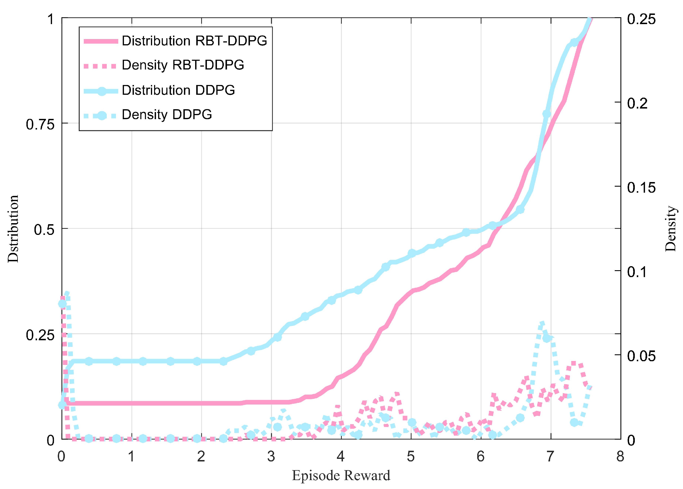
4.3. Test Results and Analysis

A Monte Carlo test was performed to verify that the strategies learned by the neural network are universally adaptable. In addition, some cases were used to analyze the anti-interception strategies. As the final performance obtained by RBT-DDPG and RBT-TD3 is similar, due to space limitations, this section uses the AN learned by RBT-DDPG as the test object.

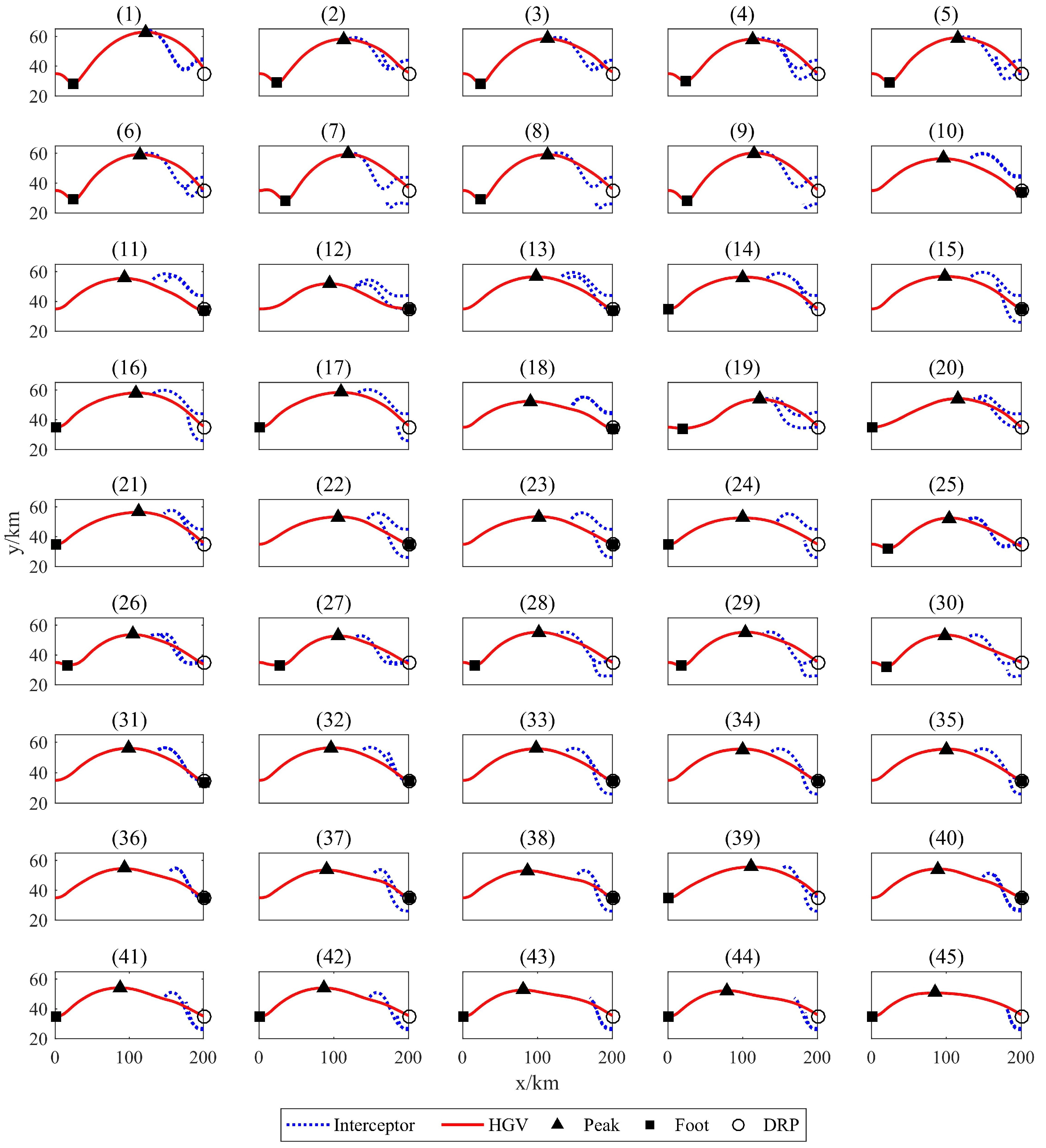
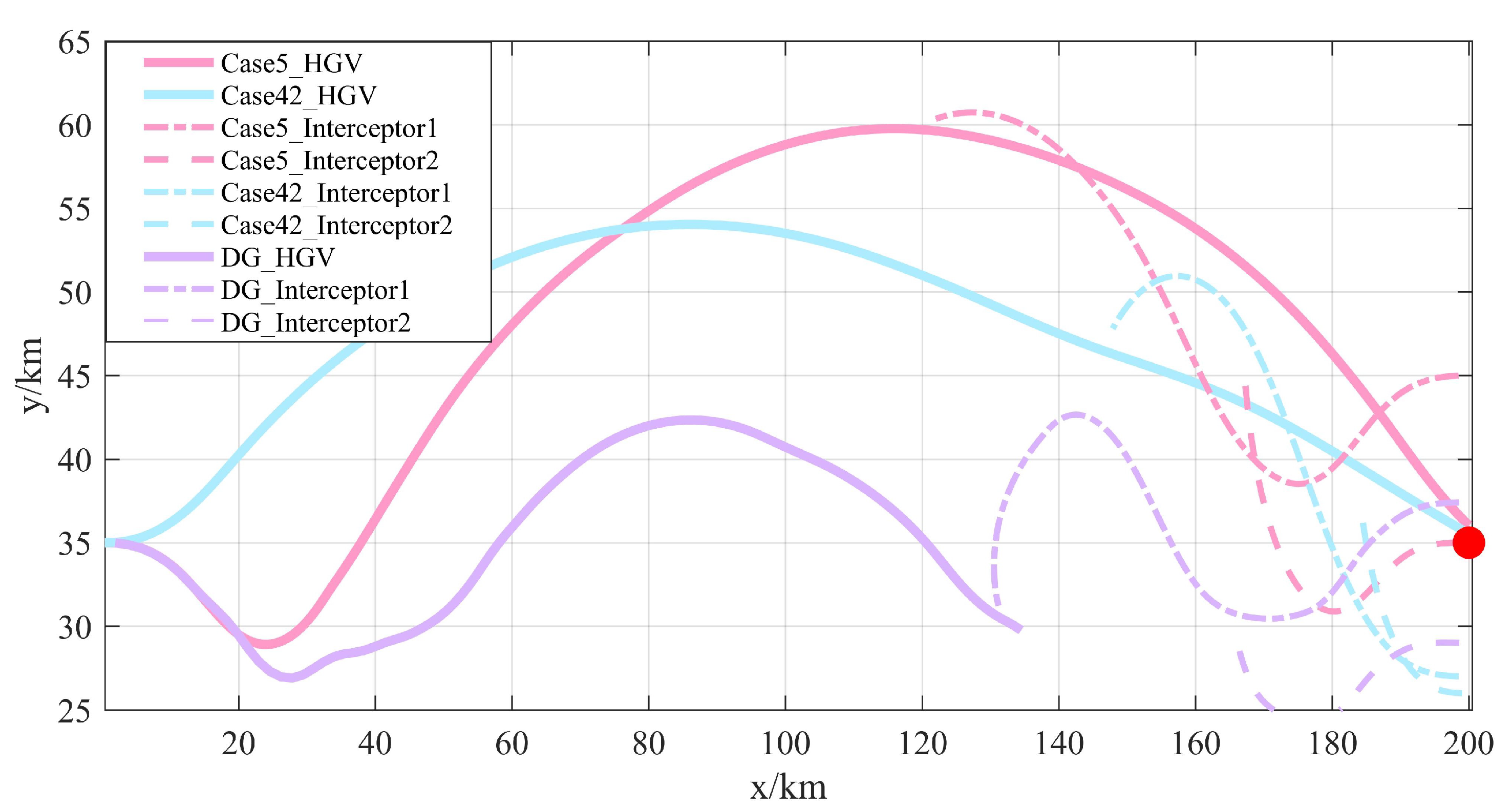
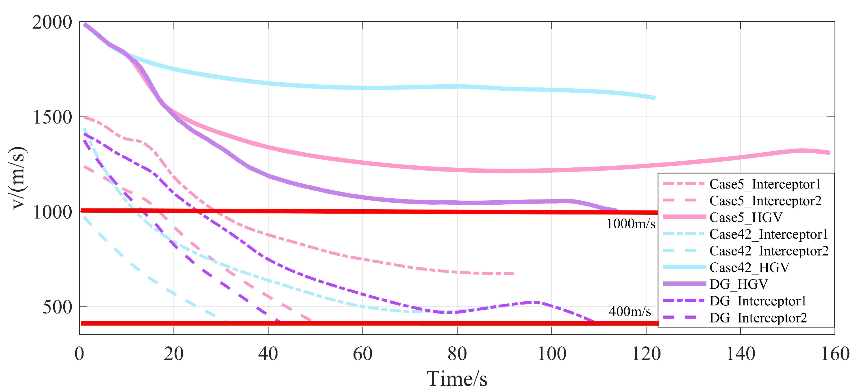
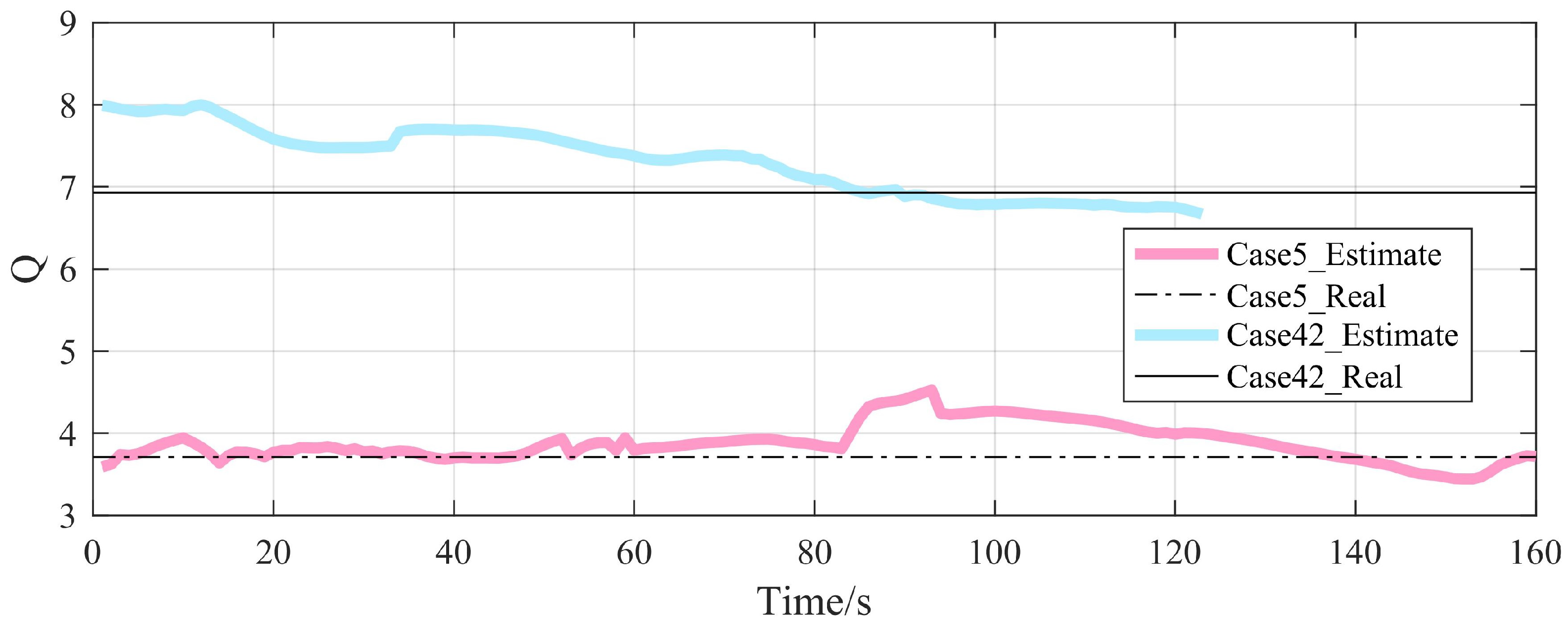
4.3.1. Monte Carlo Test

To reveal the specific strategy that was obtained from training, AN from RBT-DDPG controls an HGV in virtual scenarios to perform anti-interception tests. To verify the adaptability of an AN facing different initial states, a test was conducted using scenarios in which the initial altitude and velocity of the interceptors were randomly distributed (the same distribution as used during training). Since exploration is no longer needed, no further OU processes were added to AN. A total of 1000 episodes were conducted.

AN from DDPG and RBT-DDPG were tested for 1000 episodes each.

Table 3. Statistical results.

Algorithm	Anti-Interception Success Rate	$\overline{\mathit{e}}\left({\mathit{t}}_f\right)$/m	$\overline{\mathit{v}}\left({\mathit{t}}_f\right)$/(m/s)
DDPG	79.74%	1425.62	1377.17
RBT-DDPG	91.48%	1514.44	1453.81

and Figure 7 illustrate the results. Suppose that the measure of the success of an anti-interception is whether it eliminates two interceptors. In that case, the 91.48% anti-interception success rate of the RBT-DDPG AN is better than the 79.74% rate of the DDPG AN, reflecting the greater adaptability of the RBT-DDPG AN to complex initial conditions. According to the average terminal miss distance $\overline{e}\left(t_{\mathrm{f}}\right)$, having eliminated the interceptors, both two actors perform well in achieving DRP regression. However, on average, in terms of terminal velocity $\overline{v}\left(t_{\mathrm{f}}\right)$, the HGV guided by AN from RBT-DDPG is faster. For RBT-DDPG, the peak probability density is 7.4, while for DDPG, the peak probability density is 6.7, indicating that RBT-DDPG can perform well in more scenarios than DDPG.

To observe the specific strategies learned through RBT-DDPG, we traversed the initial conditions of the two interceptors and tested each individually. In Figure 8, the correspondence between the initial state of the interceptors and the test case serial number is indicated. The vertical motion of the HGV and interceptors in all cases are shown in Figure 9.

In Figure 9, the neural network adopts different strategies in response to interceptors with variable initial energies. In terms of behaviour, the strategies fall into two categories: S-curve (dive–leap–dive) and C-curve (leap–dive). There is also a specific pattern to the peaks. In general, the higher the initial energy of the interceptors faced by the HGV, the higher the peak.

4.3.2. Analysis of Anti-Interception Strategies

Using the data from the 5th and 42nd test cases mentioned in Section 4.3.1, we attempted to identify the strategies the neural network learned from DRL.

As shown by the solid purple trajectory in Figure 10 and Figure 11, we also used the Differential Game (DG) approach [33] as a comparison method. While the HGV evaded the interceptor with DG guidance, it lost significant kinetic energy due to its long residence in the dense atmosphere and its low ballistic dive point, and fell below the minimum velocity at approximately 55 km from the target. The DG approach uses the relative angle and velocity information as input to guide the flight, and can successfully evade the interceptor. In contrast, DG cannot account for atmospheric density and cannot optimize energy, which is a significant advantage of DRL.

The neural network chooses to dive before leaping in Case 5, whereas, in Case 42, it takes a direct leap. Furthermore, while the peak in Case 5 is 60 km, it only reaches 54 km in Case 42 before diving. In both cases, the HGV causes one of the interceptors to go below the minimum flight speed (400 m/s) before entering the rendezvous phase. At the rendezvous phase, the minimum distances between the interceptor and the HGV are 389 m and 672 m, respectively, which indicates that the HGV is almost within the interceptable area of interceptors. The terminal velocity of the HGV in Case 5 is approximately 100 m/s lower than that in Case 42, due to the higher initial interceptor energy faced in Case 5, which resulted in a longer manoeuvre path and a more violent pull-up in the dense atmospheric region. Figure 12 illustrates that the HGV tends to perform a large overload manoeuvre in the approach phase, almost exclusively utilizing the manoeuvring ability. In the regress phase of Case 42, only very small magnitude manoeuvres were required to correct the ballistic inclination, demonstrating that the neural network can control the HGV and select the appropriate ballistic inclination for the dive after escaping the interceptor.

We derived a rudimentary instant reward function with no prior knowledge of the strategy that should be implemented, resulting in a sparse reward problem. The RBT-DDPG trained a CN; however, it does not make significant Q estimation errors. There was an accurate Q estimation at the beginning of an episode, and accuracy was maintained throughout the processes, in both case 5 and case 42 (Figure 13). This phenomenon is consistent with the idea presented in Equation (12) that the flight states of both sides at the outset determine the optimal anti-interception strategy that the HGV should implement.

Figure 10, Figure 11 and Figure 12 illustrate the anti-interception strategy learned by the RBT-DDPG:(1) The HGV lures interceptors with high initial energy into dense atmospheres by diving manoeuvres in the approach phase, thus relying on pull-up manoeuvres with a denser atmosphere to drain much of the interceptors’ energy. It is important to note that this dive manoeuvre also consumes the kinetic HGV energy (e.g., Case 5). In contrast, when confronted with interceptors with low initial energy, the neural network does not choose to dive first, even though this strategy is feasible, but instead leaps directly into the thin-atmosphere region (e.g., Case 42), reflecting the optimality of the strategy. (2) Through the approach phase manoeuvre, the HGV reduces the kinetic energy of the interceptors to a proper level and attracts interceptors to the thin atmosphere. Here, the interceptor’s AO no longer supports the interceptable area to cover the whole reachable area of the HGV, which allows for the HGV to gain an available penetration path, as shown in Figure 14.

5. Conclusions

Traditionally, research on anti-interception guidance for aircraft has focused on differential game theory and optimization algorithms. Due to the high number of matrix calculations needed, applying differential game theory online is computationally uneconomic. Even though the newly developed ADP algorithm employs a neural network that significantly reduces the computation associated with the Hamilton functions, it cannot be applied to aircraft with very large flight envelopes, such as HGVs. It is challenging to implement convex planning, sequential quadratic planning, or other planning algorithms for HGVs due to their high computational complexity and insufficient real-time performance.

We conceptualize the penetration strategy of HGVs as a GTAO problem using the perspective of the optimal problem, revealing the significant impact that both the initial conditions of the attackers and defenders have on the penetration strategy. The problem is then modelled as an MDP and solved using the DDPG algorithm. The RBT-DDPG algorithm was developed to improve the CN estimation during the training process. At the end of the paper, the data on the training process and online simulation tests verify that RBT-DDPG can autonomously learn anti-interception guidance and adopt a rational strategy (S-curve or C-curve) when interceptors have differing initial energy conditions. Compared to the traditional DDPG algorithm, our proposed algorithm reduces the training episodes by 48.48%. Since the AN deployed online is straightforward, it is suitable for onboard computers. To our knowledge, this is the first to apply DRL to achieve anti-interception guidance for HGVs.

This paper focuses on a scenario in which one HGV breaks through the defences of two interceptors; this is a traditional scenario but may not be fully adapted to the future trends in group confrontation. In the future, we anticipate using multi-agent-DRL (MA-DRL) applied to multiple HGVs. The intelligent trained by MADRL can conduct guidance for each HGV in a distributed manner with limited information constraints, so the anti-intercept guidance strategy can adapt to the numbers of enemies and HGVs. This will greatly improve the intelligent generalizability to the battlefield. Additionally, RL is known to suffer from long training times. We anticipate using pseudo-spectral methods to create a collection of expert data and then combining some expert advice [43,44] to accelerate training.

References

1. Guo, Y.; Gao, Q.; Xie, J.; Qiao, Y.; Hu, X. Hypersonic vehicles against a guided missile: A defender triangle interception approach. In Proceedings of the 2014 IEEE Chinese Guidance, Navigation and Control Conference, Yantai, China, 8–10 August 2014; pp. 2506–2509. [Google Scholar]
2. Liu, K.F.; Meng, H.D.; Wang, C.J.; Li, J.; Chen, Y. Anti-Head-on Interception Penetration Guidance Law for Slide Vehicle. Mod. Def. Technol. 2008, 4, 39–45. [Google Scholar]
3. Luo, C.; Huang, C.Q.; Ding, D.L.; Guo, H. Design of Weaving Penetration for Hypersonic Glide Vehicle. Electron. Opt. Control 2013, 7, 67–72. [Google Scholar]
4. Zhu, Q.G.; Liu, G.; Xian, Y. Simulation of Reentry Maneuvering Trajectory of Tactical Ballistic Missile. Tactical Missile Technol. 2008, 1, 79–82. [Google Scholar]
5. He, L.; Yan, X.D.; Tang, S. Guidance law design for spiral-diving maneuver penetration. Acta Aeronaut. Astronaut. Sin. 2019, 40, 188–202. [Google Scholar]
6. Zhao, K.; Cao, D.Q.; Huang, W.H. Manoeuvre control of the hypersonic gliding vehicle with a scissored pair of control moment gyros. Sci. China Technol. 2018, 61, 1150–1160. [Google Scholar] [CrossRef]
7. Zhao, X.; Qin, W.W.; Zhang, X.S.; He, B.; Yan, X. Rapid full-course trajectory optimization for multi-constraint and multi-step avoidance zones. J. Solid Rocket. Technol. 2019, 42, 245–252. [Google Scholar]
8. Wang, P.; Yang, X.L.; Fu, W.X.; Qiang, L. An On-board Reentry Trajectory Planning Method with No-fly Zone Constraints. Missiles Space Vechicles 2016, 2, 1–7. [Google Scholar]
9. Fang, X.L.; Liu, X.X.; Zhang, G.Y.; Wang, F. An analysis of foreign ballistic missile manoeuvre penetration strategies. Winged Missiles J. 2011, 12, 17–22. [Google Scholar]
10. Sun, S.M.; Tang, G.J.; Zhou, Z.B. Research on Penetration Maneuver of Ballistic Missile Based on Differential Game. J. Proj. Rocket. Missiles Guid. 2010, 30, 65–68. [Google Scholar]
11. Imado, F.; Miwa, S. Fighter evasive maneuvers against proportional navigation missile. J. Aircr. 1986, 23, 825–830. [Google Scholar] [CrossRef]
12. Zhang, G.; Gao, P.; Tang, Q. The Method of the Impulse Trajectory Transfer in a Different Plane for the Ballistic Missile Penetrating Missile Defense System in the Passive Ballistic Curve. J. Astronaut. 2008, 29, 89–94. [Google Scholar]
13. Wu, Q.X.; Zhang, W.H. Research on Midcourse Maneuver Penetration of Ballistic Missile. J. Astronaut. 2006, 27, 1243–1247. [Google Scholar]
14. Zhang, K.N.; Zhou, H.; Chen, W.C. Trajectory Planning for Hypersonic Vehicle With Multiple Constraints and Multiple Manoeuvreing Penetration Strategies. J. Ballist. 2012, 24, 85–90. [Google Scholar]
15. Xian, Y.; Tian, H.P.; Wang, J.; Shi, J.Q. Research on intelligent manoeuvre penetration of missile based on differential game theory. Flight Dyn. 2014, 32, 70–73. [Google Scholar]
16. Sun, J.L.; Liu, C.S. An Overview on the Adaptive Dynamic Programming Based Missile Guidance Law. Acta Autom. Sin. 2017, 43, 1101–1113. [Google Scholar]
17. Sun, J.L.; Liu, C.S. Distributed Fuzzy Adaptive Backstepping Optimal Control for Nonlinear Multimissile Guidance Systems with Input Saturation. IEEE Trans. Fuzzy Syst. 2019, 27, 447–461. [Google Scholar]
18. Sun, J.L.; Liu, C.S. Backstepping-based adaptive dynamic programming for missile-target guidance systems with state and input constraints. J. Frankl. Inst. 2018, 355, 8412–8440. [Google Scholar] [CrossRef]
19. Wang, F.; Cui, N.G. Optimal Control of Initiative Anti-interception Penetration Using Multistage Hp-Adaptive Radau Pseudospectral Method. In Proceedings of the 2015 2nd International Conference on Information Science and Control Engineering, Shanghai, China, 24–26 April 2015. [Google Scholar]
20. Liu, Y.; Yang, Z.; Sun, M.; Chen, Z. Penetration design for the boost phase of near space aircraft. In Proceedings of the 2017 36th Chinese Control Conference, Dalian, China, 26–28 July 2017. [Google Scholar]
21. Marcus, G. Innateness, alphazero, and artificial intelligence. arXiv 2018, arXiv:1801.05667. [Google Scholar]
22. Silver, D.; Schrittwieser, J.; Simonyan, K.; Antonoglou, I.; Huang, A.; Guez, A.; Hubert, T.; Baker, L.; Lai, M.; Bolton, A.; et al. Mastering the game of go without human knowledge. Nature 2017, 550, 354–359. [Google Scholar] [CrossRef]
23. Osband, I.; Blundell, C.; Pritzel, A.; Van Roy, B. Deep Exploration via Bootstrapped DQN. arXiv 2016, arXiv:1602.04621. [Google Scholar]
24. Chen, J.W.; Cheng, Y.H.; Jiang, B. Mission-Constrained Spacecraft Attitude Control System On-Orbit Reconfiguration Algorithm. J. Astronaut. 2017, 38, 989–997. [Google Scholar]
25. Dong, C.; Deng, Y.B.; Luo, C.C.; Tang, X. Compression Artifacts Reduction by a Deep Convolutional Network. In Proceedings of the 2015 IEEE International Conference on Computer Vision, Santiago, Chile, 7–13 December 2015. [Google Scholar]
26. Fu, X.W.; Wang, H.; Xu, Z. Research on Cooperative Pursuit Strategy for Multi-UAVs based on DE-MADDPG Algorithm. Acta Aeronaut. Astronaut. Sin. 2021, 42, 311–325. [Google Scholar]
27. Brian, G.; Kris, D.; Roberto, F. Adaptive Approach Phase Guidance for a Hypersonic Glider via Reinforcement Meta Learning. In Proceedings of the AIAA SCITECH 2022 Forum, San Diego, CA, USA, 3–7 January 2022. [Google Scholar]
28. Wen, H.; Li, H.; Wang, Z.; Hou, X.; He, K. Application of DDPG-based Collision Avoidance Algorithm in Air Traffic Control. In Proceedings of the ISCID 2019: IEEE 12th International Symposium on Computational Intelligence and Design, Hangzhou, China, 14 December 2020. [Google Scholar]
29. Lin, G.; Zhu, L.; Li, J.; Zou, X.; Tang, Y. Collision-free path planning for a guava-harvesting robot based on recurrent deep reinforcement learning. Comput. Electron. Agric. 2021, 188, 106350. [Google Scholar] [CrossRef]
30. Lin, Y.; Mcphee, J.; Azad, N.L. Anti-Jerk On-Ramp Merging Using Deep Reinforcement Learning. In Proceedings of the IVS 2020: IEEE Intelligent Vehicles Symposium, Las Vegas, NV, USA, 19 October–13 November 2020. [Google Scholar]
31. Xu, X.L.; Cai, P.; Ahmed, Z.; Yellapu, V.S.; Zhang, W. Path planning and dynamic collision avoidance algorithm under COLREGs via deep reinforcement learning. Neurocomputing 2021, 468, 181–197. [Google Scholar] [CrossRef]
32. Lei, H.M. Principles of Missile Guidance and Control. Control Technol. Tactical Missile 2007, 15, 162–164. [Google Scholar]
33. Cheng, T.; Zhou, H.; Dong, X.F.; Cheng, W.C. Differential game guidance law for integration of penetration and strike of multiple flight vehicles. J. Beijing Univ. Aeronaut. Astronaut. 2022, 48, 898–909. [Google Scholar]
34. Zhao, J.S.; Gu, L.X.; Ma, H.Z. A rapid approach to convective aeroheating prediction of hypersonic vehicles. Sci. China Technol. Sci. 2013, 56, 2010–2024. [Google Scholar] [CrossRef]
35. Sutton, R.S.; Barto, A.G. Reinforcement Learning: An Introduction; MIT Press: Cambridge, MA, USA, 1998. [Google Scholar]
36. Liu, R.Z.; Wang, W.; Shen, Y.; Li, Z.; Yu, Y.; Lu, T. An Introduction of mini-AlphaStar. arXiv 2021, arXiv:2104.06890. [Google Scholar]
37. Deka, A.; Luo, W.; Li, H.; Lewis, M.; Sycara, K. Hiding Leader’s Identity in Leader-Follower Navigation through Multi-Agent Reinforcement Learning. arXiv 2021, arXiv:2103.06359. [Google Scholar]
38. Xiong, J.-H.; Tang, S.-J.; Guo, J.; Zhu, D.-L. Design of Variable Structure Guidance Law for Head-on Interception Based on Variable Coefficient Strategy. Acta Armamentarii 2014, 35, 134–139. [Google Scholar]
39. Jiang, L.; Nan, Y.; Li, Z.H. Realizing Midcourse Penetration With Deep Reinforcement Learning. IEEE Access 2021, 9, 89812–89822. [Google Scholar] [CrossRef]
40. Li, B.; Yang, Z.P.; Chen, D.Q.; Liang, S.Y.; Ma, H. Maneuvering target tracking of UAV based on MN-DDPG and transfer learning. Def. Technol. 2021, 17, 457–466. [Google Scholar] [CrossRef]
41. Wang, J.; Zhang, R. Terminal guidance for a hypersonic vehicle with impact time control. J. Guid. Control Dyn. 2018, 41, 1790–1798. [Google Scholar] [CrossRef]
42. Ge, L.Q. Cooperative Guidance for Intercepting Multiple Targets by Multiple Air-to-Air Missiles. Master’s Thesis, Nanjing University of Aeronautics and Astronautics, Nanjing, China, 2019. [Google Scholar]
43. Cruz, F.; Parisi, G.I.; Twiefel, J.; Wermter, S. Multi-modal integration of dynamic audiovisual patterns for an interactive reinforcement learning scenario. In Proceedings of the RSJ 2016: IEEE International Conference on Intelligent Robots & Systems, Daejeon, Korea, 9–14 October 2016. [Google Scholar]
44. Bignold, A.; Cruz, F.; Dazeley, R.; Vamplew, P.; Foale, C. Human engagement providing evaluative and informative advice for interactive reinforcement learning. Neural Comput. Appl. 2022. [Google Scholar] [CrossRef]
Figure 1. Illustration of an HGV anti-interception manoeuvre. The anti-interception of an HGV can be divided into three phases. ①Approach. The HGV manoeuvres according to anti-interception guidance, while the interceptor operates under its own guidance. Since the HGV is located a long distance from the interceptor, and has high energy, various penetration strategies are available during this phase. ②Endezvous. At this phase, the distance between the HGV and the interceptors is the shortest. This distance may be shorter than the kill radius of the interceptors, allowing for the HGV to be intercepted, or greater than the kill radius, allowing for the HGV to successfully avoid interception. ③Egress. With its remaining energy, the HGV flies to the DRP after moving away from the interceptors. A successful mission requires the HGV to arrive at the DRP with the highest levels of energy and accuracy. From the above analysis, it can be seen that whether the HGV can evade the interceptors in phase ② depends on the manoeuvres adopted in phase ①. Phase ① also determines the difficulty of ballistic regression in phase ③.
Aerospace 09 00424 g001
Figure 2. Signal flow of the RBT-DDPG algorithm. When a sample batch is used to update the CN parameters, the CN is repetitively trained using the loss function as its reference threshold (as shown in Steps 4–7 of the Figure), thereby avoiding a serious misestimate of CN.
Aerospace 09 00424 g002
Figure 3. Structures of the neural networks ((Left) AN. (Right) CN) with theparameters of each layer.
Aerospace 09 00424 g003
Figure 4. Cumulative reward during training. With the help of the RBT mechanism, both DDPG and TD3 reached a faster training speed.
Aerospace 09 00424 g004
Figure 5. Loss function of AN and CN during training. Similar to the cumulative reward curve presented in Figure 4, the actor loss function of RBT-DDPG in Figure 5 decreases faster, indicating that RBT-DDPG ensures that AN learns faster. RBT-DDPG has a lower CN loss function almost throughout the episodes, reflecting that RBT can improve the CN estimation. The same phenomenon occurs in the comparison between RBT-TD3 and its original version.
Aerospace 09 00424 g005
Figure 6. The number of RBT iterations that occur during RBT-DDPG training. RBT is repeated several times at the beginning of training (near the first training iteration), and CN is required to train to a tiny estimation error. RBT is barely executed before 60,000 training steps, as CN can already provide accurate estimates for the samples in the current memory pool, and no additional training is needed. From steps 100,000 to 200,000, RBT is repeated several times, and many of the executions are greater than 10. Due to the introduction of new strategies into the memory pool, the original CN does not accurately estimate the Q value, so additional training is performed. Between steps 20,000 and 35,000, RBT is occasionallyexecuted, and most executions contain less than 10 repetitions because fine-tuning CN can accommodate the new strategies that are explored by the actor. RBT executions increase after 350,000 steps, as CN must adapt to the multiple strategy samples brought into the memory pool. At the end of training, the average -number of repetitions is approximately 2, which is an acceptable algorithmic complexity cost.
Aerospace 09 00424 g006
Figure 7. Probability distribution and density of the cumulative reward for each episode in the Monte Carlo test. About 10% of the RBT-DDPG rewards are less than 3, compared to about 24% of DDPG reflecting the greater adaptability of the RBT-DDPG AN to complex initial conditions.
Aerospace 09 00424 g007
Figure 8. Correspondence between initial state and test case serial number (the horizontal coordinate represents the initial state of the first interceptor, while the vertical coordinate represents the second interceptor. The letters M, H, and L in the first position represent 44 km, 35 km, and 26 km altitude, respectively. The letters M, H, and L in the second position represent 1500 m/s, 1250 m/s, and 1000 m/s velocities, respectively).
Aerospace 09 00424 g008
Figure 9. Vertical motion of the HGV and interceptors in the test cases. The strategies fall into two categories: S-curve (dive–leap–dive) and C-curve (leap–dive). There is also a specific pattern to the peaks.
Aerospace 09 00424 g009
Figure 10. Vertical motion comparison between RBT-DDPG(Cases 5 and 42) and Differential Game. The DG approach uses the relative angle and velocity information as input to guide the flight, and can successfully evade the interceptor. In contrast, DG cannot account for atmospheric density and cannot optimize energy, which is a significant advantage of DRL. The AN learned by RBT-DDPG chooses to dive before leaping in Case 5, whereas, in Case 42, it takes a direct leap. Furthermore, while the peak in Case 5 is 60 km, it only reaches 54 km in Case 42 before diving. The AN can control the HGV to select the appropriate ballistic inclination for the dive after escaping the interceptor.
Aerospace 09 00424 g010
Figure 11. Velocities comparison between RBT-DDPG(Cases 5 and 42) and Differential Game.
Aerospace 09 00424 g011
Figure 12. Overloads comparison between Cases 5 and 42.
Aerospace 09 00424 g012
Figure 13. Q-value comparison between Case 5 and 42, as shown in Figure 12. An accurate Q estimation at the beginning of an episode and maintains accuracy throughout the processes in both case 5 and case 42.
Aerospace 09 00424 g013
Figure 14. Illustration of the penetration strategy during the rendezvous phase learned by RBT-DDPG. The interceptor’s AO no longer supports the interceptable area to cover the whole reachable area of the HGV, which allows for the HGV to gain an available penetration path.
Aerospace 09 00424 g014