A Prognostic and Health Management Framework for Aero-Engines Based on a Dynamic Probability Model and LSTM Network

Abstract

In this study, a prognostics and health management (PHM) framework is proposed for aero-engines, which combines a dynamic probability (DP) model and a long short-term memory neural network (LSTM). A DP model based on Gaussian mixture model-adaptive density peaks clustering algorithm, which has the advantages of an extremely short training time and high enough precision, is employed for modelling engine fault development from the beginning of engine service, and principal component analysis is introduced to convert complex high-dimensional raw data into low-dimensional data. The model can be updated from time to time according to the accumulation of engine data to capture the occurrence and evolution process of engine faults. In order to address the problems with the commonly used data driven methods, the DP + LSTM model is employed to estimate the remaining useful life (RUL) of the engine. Finally, the proposed PHM framework is validated experimentally using NASA’s commercial modular aero-propulsion system simulation dataset, and the results indicate that the DP model has higher stability than the classical artificial neural network method in fault diagnosis, whereas the DP + LSTM model has higher accuracy in RUL estimation than other classical deep learning methods.

1. Introduction

Aero-engines are core machinery systems with complex structures, high levels of integration and poor working conditions, of which the reliable and efficient operations are crucial to the flight safety of aircraft. Prognostics and health management (PHM) is an effective maintenance technique to achieve safe and reliable operations of machines and systems, and plays a significant role in the operations of aero-engines [1,2,3]. Incomplete statistics showed that failures of gas path components account for more than 90% of all engine failures, 60% of the aero-engine maintenance costs are spent on gas-path components [4]. However, due to the unique manufacturing technologies and special materials of the aero-engine, it is difficult to maintain and replace the components of engines frequently [5]. The PHM system is capable of determining whether a gas-path component has failed and deciding whether it needs to be repaired or replaced, thus can reduce routine maintenance costs and time. Fault diagnosis and remaining useful life (RUL) estimation are research emphases of PHM.

In general, PHM approaches can be categorized into model-based methods [6,7] and data-driven methods [8,9]. Model-based methods include physical models, structural analysis, contact analysis cumulative damage models, cyclic fatigue, and crack propagation models, etc., [10]. Obviously, they need a detailed mathematical model of the aero-engine [11]. In addition, their reliability decreases as the system nonlinearities, complexity, and modeling uncertainties increase. Data-driven methods can be roughly divided into two categories, namely machine learning algorithms and probability models, and they do not require deep knowledge of the engine mechanism, and mostly depend on real-time or collected historical data from the engine sensors and measurements, so they have attracted considerable attention and have been developed rapidly. Commonly used data-driven methods include artificial neural network (ANN), support vector machine (SVM), k-means clustering algorithm, Bayesian method, Markov model, Gaussian distribution, etc. [12,13,14,15,16,17,18].

The operation and external conditions of aero-engine change over time and, therefore, the time-varying problems, have become the main challenge. Machine learning can be used for fault diagnosis, but it is not flexible enough to deal with time-varying problems and is difficult to update as data accumulates. The traditional ANN is also known as the black box model. Its construction process does not reflect the actual operation law of the engine. In addition, it has the limitations of weak generalization ability and difficulty in dealing with time-varying problems, etc. Chen et al. [1] proposed a new deep learning method called deep belief network (DBN) for engine fault diagnosis. Compared with the traditional back propagation (BP) model, it has been greatly improved, but its essence is still ANN, which has the above-mentioned drawbacks. Compared with ANN, the probability model has unique advantages in dealing with time-varying problems due to its solid mathematical background. The Gaussian mixture model (GMM) is a typical probability model, which can fit the fault monitoring features (FMFs) of random distribution by a combination of a finite number of Gaussian components (GCs) [19]. Avendaño Valencia et al. [20] proposed a stochastic framework based on the Gaussian mixture random coefficient model for structural health state monitoring under time-varying conditions, and their results showed that GMM has great flexibility in dealing with time-varying and uncertain problems. Qiu et al. [21] proposed an enhanced dynamic Gaussian mixture model-based damage monitoring method for aircraft structural health monitoring (SHM). Fang et al. [22] proposed a probability modeling-based aircraft structural health monitoring framework under time-varying conditions.

However, the probability model is rarely used in aero-engine PHM systems, especially the GMM model. The difficulty of applying the probability model to aero-engines lies in the data of aero-engine contain noise, which is much more complex than those of other objects such as aircraft structural analysis [23]. In addition, the biggest disadvantage of the traditional GMM model is that the initial values have a great influence on the result, and manual selection is required. At present, the most common improvement is to use the k-means clustering algorithm [24], but it is still unable to achieve complete self-adaptation. A new method called adaptive density peaks clustering algorithm (ADPC) can solve these problems and realize adaptive initial clustering. Another difficulty in aero-engine fault diagnosis lies in the difficulty of obtaining a large amount of failure data for an engine. Most of the engine’s life cycle is in the non-failure state, and it is a gradual process for an engine from health to failure. Therefore, it is necessary to design a dynamic model that makes full use of the normal data and can be updated as the data accumulates.

RUL estimation is another focus in the PHM framework. Data-driven approaches are typical algorithms for RUL estimation. Soualhi et al. [25] developed a data-driven approach for bearing RUL prediction using the Hilbert–Huang transform (HHT) and the SVM. Li et al. [26] proposed a smooth transition auto-regression model combined with the Bayesian model to estimate the RUL. Listou et al. [27] proposed a semi-supervised learning method for RUL prediction, which reduced the amount of marker training data. However, these methods also suffer from some deficiencies. For instance, the imperfection of expert knowledge may cause the handcrafted feature to fail to effectively reflect the engine degradation, and these methods do not propose a good solution mechanism for the utilization of historical data and current data. In addition, the prediction accuracy of these methods is not optimal.

In the construction of the PHM framework, Che et al. [1] proposed a framework combining DBN and long short-term memory neural network (LSTM) methods. In his framework, fault diagnosis and RUL estimation are not deeply linked, and health indicators are not fully utilized in RUL estimation, which makes it necessary to mine information from engine sensor data again before RUL estimation, which is not the most efficient. Li et al. [28] proposed a framework for deriving system requirements for PHM system development to provide a solution for predicting RUL. Similarly, the framework does not consider a technical route that combines fault diagnosis with RUL estimation.

Given the above, an aero-engine PHM framework based on GMM-ADPC algorithm and LSTM network is proposed in this study. In this study, a new GMM-ADPC algorithm is proposed to construct probability distribution space of engine data. Based on the GMM-ADPC algorithm, a dynamic probability (DP) model is proposed for modeling engine fault development. This model has a solid mathematical foundation and can make full use of engine life cycle data. And principal component analysis (PCA) is used to convert complex high-dimensional raw data into low-dimensional data. For the purpose of addressing the problems with the commonly used data-driven methods, the DP + LSTM model is introduced for RUL estimation. Here, the engine fault probability distribution data constructed by the DP model is used as the input of the LSTM network, which realizes the information transmission between the two modules, avoids sensor noise interference to a certain extent, and improves the stability and accuracy of the PHM framework.

The rest of this paper proceeds as follows. Section 2 introduces the DP model and LSTM algorithms. Section 3 details the architecture and the realization of the framework. Section 4 provides the validation results of the framework in NASA’s dataset. Finally, the conclusion of this work is given in Section 5.

2. PHM Basic Theory

2.1. Probability Modeling

The core algorithm of the probability model is the GMM-ADPC algorithm, and the probability difference measuring method is used to quantify the difference between two probability models so as to generate fault detection indexes.

2.1.1. GMM-ADPC Algorithm

GMM is an extension of single Gaussian probability density function. It is a weighted sum of a finite number of GCs. Assume $X=\left[{\mathit{x}}_1,{\mathit{x}}_2,\cdot \cdot \cdot ,{\mathit{x}}_i,\cdot \cdot \cdot ,{\mathit{x}}_N\right]$ denote a feature sample set composed by N FMFs, i = 1, 2, …, N, where ${\mathit{x}}_i=\left[{\mathit{x}}_1,{\mathit{x}}_2,\cdot \cdot \cdot ,{\mathit{x}}_D\right]$ represents a FMF with D dimensionality. Equation (1) expresses the probability density function of GMM and Equation (2) expresses the GC.

$$\Phi \left({\mathit{x}}_i|\zeta \right)={\displaystyle \sum _{k=1}^K{w}_k{\phi }_k\left({\mathit{x}}_i|{\mu }_k,{\Sigma }_k\right)}$$

(1)

$${\phi }_k\left({\mathit{x}}_i|{\mu }_k,{\Sigma }_k\right)=\frac{1}{{\left(2\pi \right)}^{\frac{D}{2}}{\left|{\Sigma }_k\right|}^{\frac{1}{2}}}{e}^{-\frac{1}{2}{\left({\mathit{x}}_i-{\mu }_k\right)}^T{\Sigma }_k{}^{-1}\left({\mathit{x}}_i-{\mu }_k\right)}$$

(2)

where $\zeta =\left\{\left(w_1,{\mu }_1,{\Sigma }_1\right),\cdot \cdot \cdot ,\left(w_k,{\mu }_k,{\Sigma }_k\right),\cdot \cdot \cdot ,\left(w_K,{\mu }_K,{\Sigma }_K\right)\right\}$ is the most important parameter set of GMM. The number of GCs is K and $k=1,2,\cdot \cdot \cdot ,K$. The parameter $\zeta$, $w_k$, ${\mu }_k$ and ${\Sigma }_k$ denote the mixture weight, mean, and covariance matrix of the k-th GC, respectively, $|\cdot |$ is the determinant value, and T is the transpose.

Usually, the Expectation-Maximization (EM) algorithm is used to construct GMM [29]. However, the drawback of the EM algorithm is that the initial values of $\zeta$ will greatly affect the result, which results in reduced stability of GMM. Some methods, such as the Bayesian non-parametric clustering approach and enhanced dynamic GMM method, have been proposed to determine $\zeta$ [21,30]. However, the ideal approach is adaptive and not computationally intensive. In addition, since each sample set belongs to a different FMF, the selected method is required to have good generalization performance. In fact, GMM represents the probability distribution of FMFs, with each GC representing a cluster. ADPC is an improved clustering algorithm based on probability density distribution [31,32]. The main advantage of the ADPC algorithm is that it could effectively identify clustering centers and cut-off distances with low-dimensions or arbitrary data sets. The ADPC algorithm contains the following two main steps:

Step 1: Automatic identification of the cut-off distance.

First, define a variable H to represent the uncertainty of the system expressed as Equations (3)–(5). If the values of H are smaller, the uncertainty of the system will be smaller, which is in favor of clustering.

$$H=-{\displaystyle \sum _{i=1}^n\left({\delta }_i{\displaystyle \sum _j{e}^{-{\left(\frac{d_{ij}}{d_c}\right)}^2}}\right)}\log \left({\delta }_i{\displaystyle \sum _j{e}^{-{\left(\frac{d_{ij}}{d_c}\right)}^2}}\right)$$

(3)

$${\delta }_i=\underset{{\rho }_i<{\rho }_j}{\min }\left(d_{ij}\right)$$

(4)

$${\rho }_i={\displaystyle \sum _j{e}^{-{\left(\frac{d_{ij}}{d_c}\right)}^2}}$$

(5)

where $d_{ij}$ is the distance between FMF ${\mathit{x}}_i$ and FMF ${\mathit{x}}_j$, ${\rho }_i$ is the local density of FMF ${\mathit{x}}_i$. Make the $d_c$ gradually increase from 0 until H has the minimum value, in which case $d_c$ is the most appropriate cut-off distance.

For some samples, it is difficult to find the cut-off distance that meets the above requirements. In this case, $d_c$ can be set as the top 1% to 2% of the distance between all data points [31].

Step 2: Automatically identify clustering centers.

Clustering centers should have both large ${\rho }_i$ and ${\delta }_i$ values. Define a variable $\gamma$ expressed as Equation (6). Sample points with larger $\gamma$ values are more suitable for clustering centers.

$${\gamma }_i={\rho }_i{\delta }_i$$

(6)

In addition, the number of cluster centers needs to be determined. Firstly, calculate the $\gamma$ value of each FMF and sort them. Let $ten{d}_i$ be a criterion for determining the number of cluster centers, and $ten{d}_i$ expressed as Equation (7).

$$ten{d}_i=\left(i-1\right)\frac{{\gamma }_{i-1}-{\gamma }_i}{{\gamma }_i-{\gamma }_{i+1}}$$

(7)

Then, select the n FMFs with the largest $\gamma$ value, and calculate the $ten{d}_i$ value for each FMF. If the $ten{d}_i$ value of the m-th FMF is the largest, then the former m − 1 FMFs are taken as the clustering center.

After the initial clustering is completed, the mean, covariance, and weight of FMFs belonging to each cluster can be obtained and can be used as the initial value $\zeta$ of the EM algorithm.

2.1.2. Probability Difference Measuring Method

In this paper, two probability models are constructed, as detailed in the following sections. Appropriate rules for quantifying the difference between the two models need to be determined. Some methods such as Renyi divergence and Kullback-Leibler divergence [33] have been proposed to measure the difference. However, these methods are not symmetric and normalized. Qiu et al. [21] used the Monte Carlo simulation method in probability similarity measuring and achieved good results [34]. Firstly, let $X_{MC}=\left\{{\mathit{x}}_1,{\mathit{x}}_2,\cdot \cdot \cdot ,{\mathit{x}}_R\right\}$ denote a large number of random samples that are generated by Monte Carlo sampling. Secondly, the posterior probability of $X_{MC}$, is denoted as $P\left(X_{MC}|\zeta \right)={\left\{\Phi \left({\mathit{x}}_1|\zeta \right),\Phi \left({\mathit{x}}_2|\zeta \right),\cdot \cdot \cdot ,\Phi \left({\mathit{x}}_R|\zeta \right)\right\}}^T$, which can be calculated by Equations (1) and (2). Finally, the difference between the two probability models can be calculated by Equation (8). In this paper, $Diff\left({\zeta }_1,{\zeta }_2\right)$ actually denotes the fault detection indexes.

$$Diff\left({\zeta }_1,{\zeta }_2\right)=1-\frac{P{\left(X_{MC}|{\zeta }_1\right)}^{T}P{\left(X_{MC}|{\zeta }_2\right)}^T}{\Vert P\left(X_{MC}|{\zeta }_1\right)\Vert \cdot \Vert P\left(X_{MC}|{\zeta }_2\right)\Vert }$$

(8)

2.2. Long Short-Term Memory Networks

LSTM model based recurrent neural network (RNN) can adaptively learn the representative information through multiple non-linear transformations [35,36,37]. Compared with the traditional ANN, LSTM can remember all the historical information entered and is suitable for dealing with time-varying problems. Compared with RNN, LSTM has been improved in two main aspects. First, in order to solve the limitation of information forgetting, the cell state is split into the short-term state ${\mathit{h}}_t$ and the long-term state ${\mathit{c}}_t$. Second, the cell states are regulated by three control gates, the forget gate, the input gate, and the output gate [38]. The architecture of LSTM can be described in Figure 1.

A typical LSTM is illustrated in Figure 1, and the hidden layer contains three gates: forget gate, input gate, and output gate. The functions of these three gates are: information forgetting, long-term state updating, and short-term state updating.

• Information forgetting. The states removed from the previous long-term state ${\mathit{c}}_{t-1}$ are controlled by the forget gate ${\mathit{f}}_t$. The ${\mathit{f}}_t$ can be described by Equation (9).

  $${\mathit{f}}_t=\sigma \left({\mathit{w}}_f\cdot \left[{\mathit{h}}_{t-1},{\mathit{x}}_t\right]+{\mathit{b}}_f\right)$$

  (9)

  where $\sigma$ is the sigmoid function, ${\mathit{x}}_t$ is the previous current time, ${\mathit{w}}_f$ is the weight vectors, ${\mathit{b}}_f$ is the bias term of the forget gate, and “$\cdot$” means matrix multiplication.
• Long-term state updating. The input gate layer determines what values will be updated. The input gate ${\mathit{i}}_t$ and candidate value vector ${\mathit{c}}_t^{\prime }$ are expressed by Equations (10) and (11).

  $${\mathit{i}}_t=\sigma \left({\mathit{w}}_i\cdot \left[{\mathit{h}}_{t-1},{\mathit{x}}_t\right]+{\mathit{b}}_i\right)$$

  (10)

  $${\mathit{c}}_t^{\prime }=\mathrm{Tanh}\left({\mathit{w}}_c\cdot \left[{\mathit{h}}_{t-1},{\mathit{x}}_t\right]+{\mathit{b}}_c\right)$$

  (11)

  where $\left({\mathit{w}}_i,{\mathit{w}}_c\right)$ are the weight vectors, and $\left({\mathit{b}}_i,{\mathit{b}}_c\right)$ are bias terms.

Then, the new long-term cell state ${\mathit{c}}_t$ can be obtained by Equation (12).

$${\mathit{c}}_t={\mathit{f}}_t\otimes {\mathit{c}}_{t-1}\oplus {\mathit{i}}_t\otimes {\mathit{c}}_t^{\prime }$$

(12)

where $\left(\otimes ,\oplus \right)$ are element-wise multiplication and addition.

3.

Short-term state updating. The function of the output gate is to change the long-term state to the short-term state. Equation (13) describes the output gate ${\mathit{o}}_t$.

$${\mathit{o}}_t=\sigma \left({\mathit{w}}_o\cdot \left[{\mathit{h}}_{t-1},{\mathit{x}}_t\right]+{\mathit{b}}_o\right)$$

(13)

Finally, the short-term state of the cell unit at time t can be described as Equation (14).

$${\mathit{h}}_t={\mathit{o}}_t\otimes \mathrm{Tanh}\left({\mathit{c}}_t\right)$$

(14)

In this study, LSTM implements the prediction of sequential to point, the dimension of the input sequence is 10. The loss function is mean squared error (MSE), and the optimizer is the ADAM algorithm, which is an extension of the gradient descent algorithm.

3. Design of the Aero-Engine PHM Framework

3.1. DP Model for Fault Monitoring

Data collected by aero-engine sensors vary over time and contain noise [39]. Furthermore, aero-engines are designed based on failure-tolerance, which means that the engine will keep a healthy state in the early stage of the engine, and the influence of fault is minimal and even far lower than the time-varying influence. As time goes on, the influence of the fault becomes greater and greater until the engine is unable to function properly. Therefore, it is necessary to find a method that can not only eliminate the influence of noise but also capture the accumulation of engine fault. Generally, the operating state of the engine cannot be directly reflected by sensor data at a certain moment. Deriving the engine state from the physical meaning of the data itself is difficult and complex. Therefore, the core idea of the proposed framework is to construct the probability distribution of engine life cycle data, which is dynamically updated. Different health states necessarily correspond to different probability distributions. Double probability models are constructed to represent the engine health state and the health monitoring state, respectively, and the monitoring probability model must be updatable so as to reveal the progressive variation trend. Once the double probability models are constructed, the engine fault can be quantified by comparing the difference between the two probability models. It should be noted that this method is proposed on the assumption that the time-varying influences of the two states are the same.

In addition, the DP model is designed as standardized architecture. In the PHM field, some model-driven methods such as Kalman Filtering, particle filter [40], and so on are all aimed at fixed objects. When the engine model is different, the PHM model needs to be modified. Some data-driven methods such as ANN, SVM, and so on also have limited generalization capability [14,15]. In contrast to these methods, the DP model can be designed as standardized architecture that is suitable for different engine models, because the DP model is updated dynamically with the accumulation of engine data, so it does not require much prior knowledge or complex model parameter adjustment, and considering the inevitability of data transfer in the framework, the proposed PHM framework in this paper will use a generalized data interface between the parts. In addition, the input and output data of the framework are normalized. Another significant advantage of the DP model is that it does not need training as ANN does, so this method is more efficient than ANN.

3.2. Combining the DP Model and LSTM for the PHM Framework

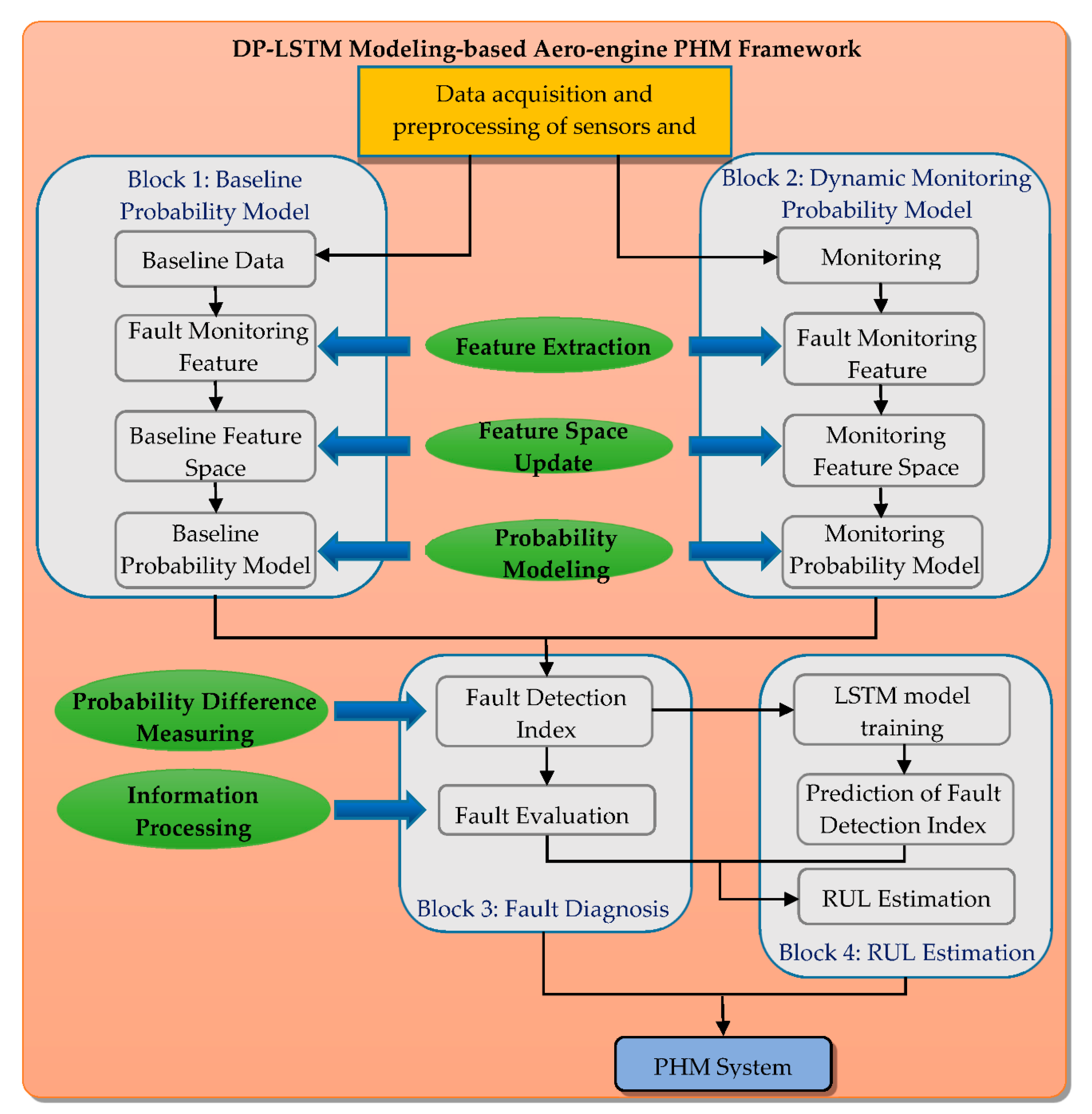
The modular hierarchical structure is a prominent feature of the proposed PHM framework, and the framework contains four blocks, as shown in Figure 2. The first step of the framework is to obtain sensors data for the entire life cycle and RUL information of the engine, which is large and contains noise. Therefore, in this step, it is necessary to clean these sensors’ data and reduce their dimensions through the PCA technique [41]. Then, the data after dimension reduction should be standardized. The preprocessed data is divided into baseline data and monitoring data, which are passed into Block 1 and Block 2, respectively. These two blocks constitute the double probability models. Block 1 constructs the baseline probability model based on the baseline data; that is, the data under the engine health state. For the same engine, the baseline probability model remains unchanged and is updated for different engines. Block 2 constructs the monitoring probability model based on real-time monitoring data, which needs to be updated in real-time. After the construction of the double probability models, the difference ($Diff\left({\zeta }_B,{\zeta }_O\right)$, where ${\zeta }_B$ and ${\zeta }_O$ are the parameters of baseline and monitoring probability models, respectively) between the two models can be used to evaluate the degree of engine failure, and that is what Block 3 does. In this paper, the normalized $Diff\left({\zeta }_B,{\zeta }_O\right)$ are used as fault detection indexes. Block 4 is the second part of the PHM framework-RUL estimation. The large amount of fault detection index data generated by the fault diagnosis module is taken as the training sample of the LSTM network. In this way, the interference of sensor data noise can be avoided. In addition, since the probability model contains the information of the entire data set, it is difficult for the fault detection indexes to be disturbed by a very small number of abnormal data. Therefore, the framework combining the two models has better stability. RUL prediction can be started from any time of different engines. A threshold value can be selected to conduct RUL evaluation according to the fault detection index curve.

4. Results and Discussions

In order to further evaluate the PHM model, a turbofan engine performance degradation dataset, which is generated by commercial modular aero-propulsion system simulation (C-MAPSS) [42], is utilized. Each example within the turbofan dataset is a time series signal of various sensor data and operating conditions data which is measured periodically over the life-cycle of the turbofans [43].

4.1. Data Sets Characterization

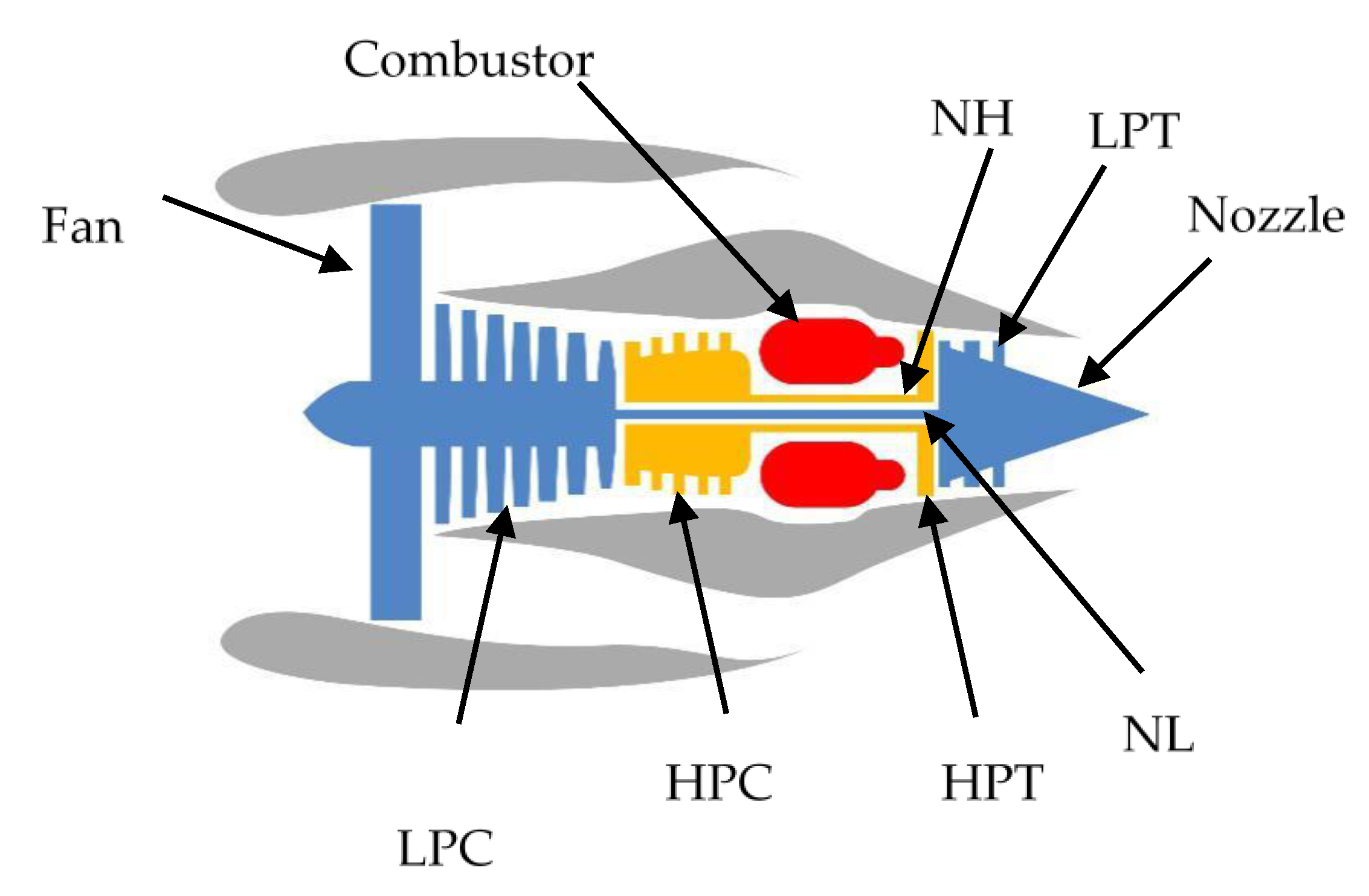
As shown in Figure 3, a turbofan engine normally includes a fan, low pressure compressor (LPC), low pressure turbine (LPT), high pressure compressor (HPC), high pressure turbine (HPT), combustor, and a nozzle. The C-MAPSS data sets are multiple multivariate time series. Each dataset has been partitioned into training and test sample sets. Each dataset (i.e., a 24-element vector) includes 21 characteristic sensors for engine health data recording. With the preprocessing method, 14 sensors that are currently available onboard for many commercial turbofan engines are selected for PHM in this study [44].

Table 1. Fourteen selected sensors in C-MAPSS.

No.	Sensor Abbreviation	Description	Units
1	T24	Total temperature at low pressure compressor outlet	${}^{\circ }R$
2	T30	Total temperature at high pressure compressor outlet	${}^{\circ }R$
3	T50	Total temperature at low pressure turbine outlet	${}^{\circ }R$
4	P30	Total pressure at high pressure compressor outlet	psia
5	Nf	Physical fan speed	rpm
6	Nc	Physical core speed	rpm
7	Ps30	Static pressure at high pressure compressor outlet (Ps30)	psia
8	Phi	Ratio of fuel flow to Ps30	pps/psi
9	NRf	Corrected fan speed	rpm
10	NRc	Corrected core speed	rpm
11	BPR	Bypass ratio	-
12	Ht Bleed	Burner fuel–air ratio	-
13	W31	High pressure turbine coolant bleed	lbm/s
14	W32	Low pressure turbine coolant bleed	lbm/s

shows the description of selected sensors.

After the raw data is selected, the Z-score method is used to standardize the 14 sensor parameters. The Z-score actually reflects the relative standard distance from an element to the mean. It can be calculated as:

$$z=\left(x-\mu \right)/\sigma$$

(15)

where z is the z-score, x is the value of the element, μ is the population mean, and σ is the standard deviation.

In this paper, four datasets (Engine #1–#4) are selected to validate the DP model, and 80 datasets (60 datasets as training samples and 20 datasets as testing samples) are selected to validate the LSTM model.

4.2. Fault Diagnosis

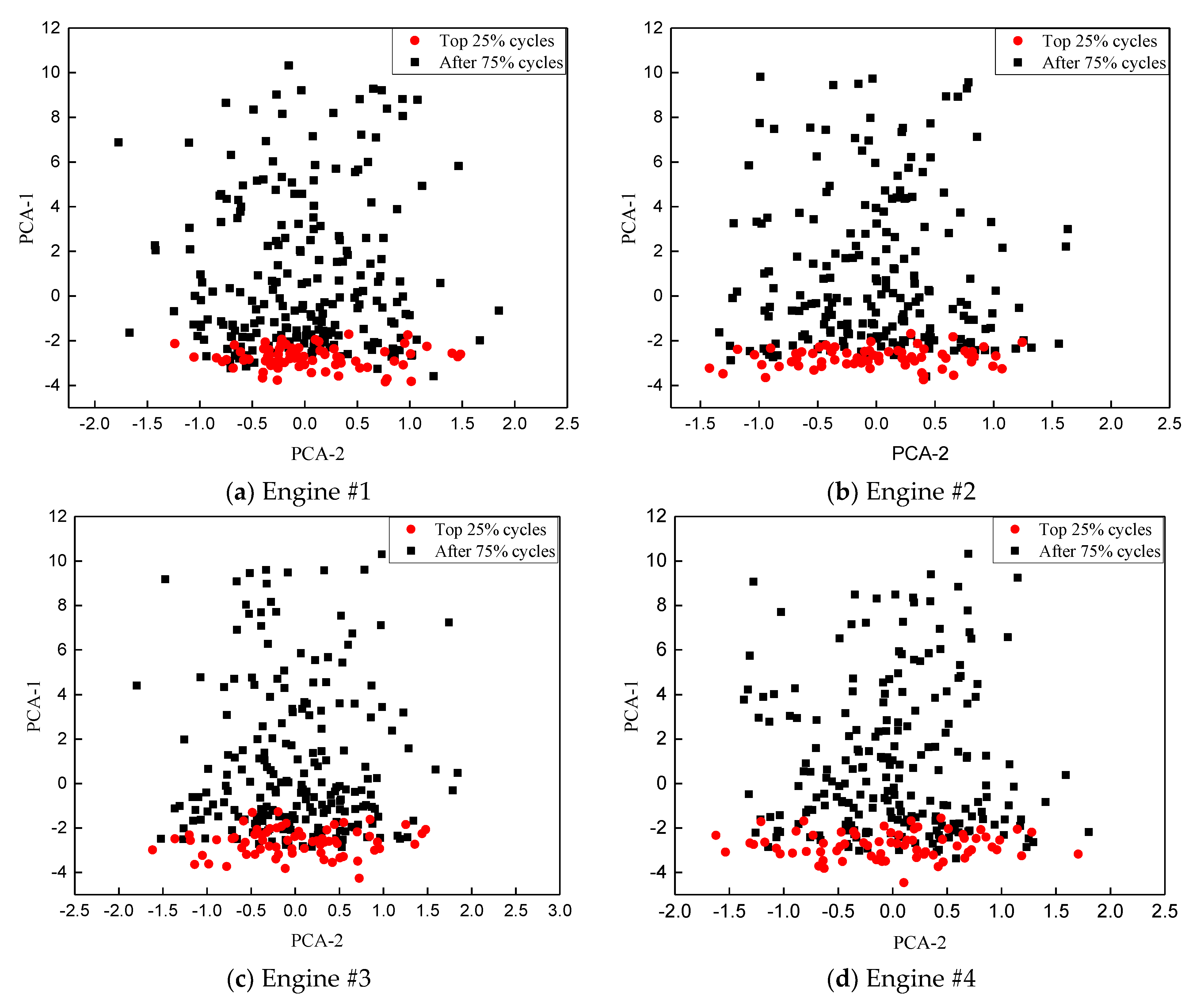
This section corresponds to Block 1, Block2, and Block3 in the PHM framework diagram. In Section 4.1, a high dimensional dataset containing 14 sensor parameters was obtained. Because of the limitation of DP model in processing high-dimensional data, PCA is used to construct a two-dimensional FMF. The data of the four engines processed by PCA is shown in Figure 4.

As can be seen in the figure, the red dots represent the data of the top 25% cycles, which are very concentrated, and there is little difference in the first principal component among the data points. Based on experience, we can assume that the engine is in a healthy state for the top 25% cycles, and the data of top 25% cycles is considered to be baseline data. Here, 25% is a conservative estimate and does not mean that the engine will fail after 25%. Figure 4 also tells us that the data for the after 75% cycles of the engine is heavily dispersed, which means that the operating data of the engine during this period has gradually deviated from the data of the health state.

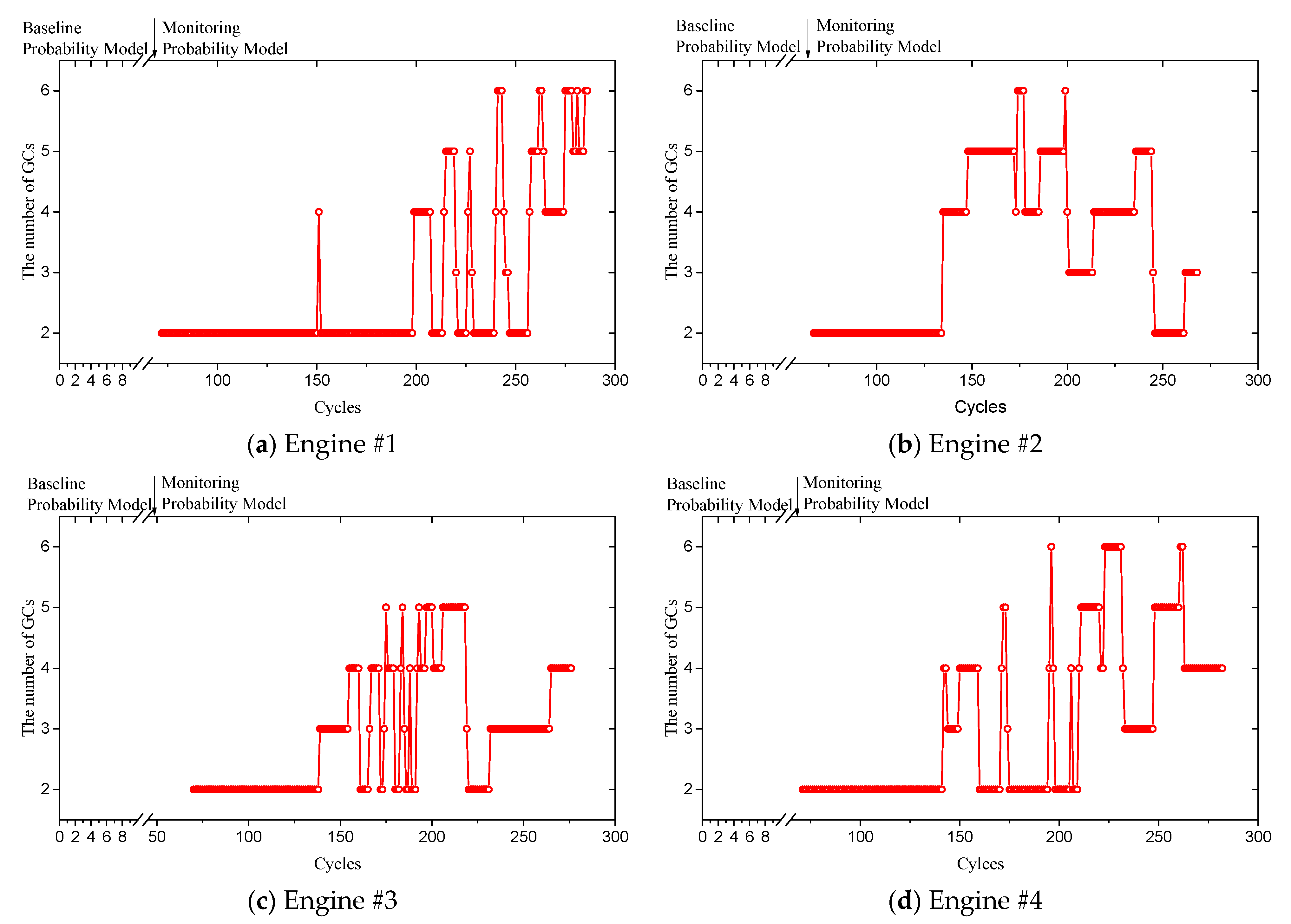
After the preprocessing of the original data is completed, the initial classification of these data can be achieved by the ADPC algorithm, so as to obtain the initial values of $\zeta$ required by the GMM. Although the ADPC algorithm can adaptively identify clustering centers and cut-off distance, the research in this paper finds that the method has limitations when dealing the sample sets with small sizes. Therefore, in the early stage of engine operation, the sample size is still small, and a limiter is added to the ADPC algorithm to keep the number of clustering centers and cut-off distance unchanged. Therefore, a fixed number of cluster centers and cut-off distance are used for the top 50% of the engine full life cycles. In addition, the number of cluster centers is set between the interval [2,6], and the difference between the number of cluster centers of two adjacent samples cannot be more than two. The idea is to prevent violent oscillations in rare cases. The above measures can ensure the accuracy and stability of the established model. The variation of the number of clustering centers in the full life cycles is shown in Figure 5. This figure reflects that the number of GCs recognized by the ADPC is changing adaptively to the changing monitoring feature space along with the engine life cycle.

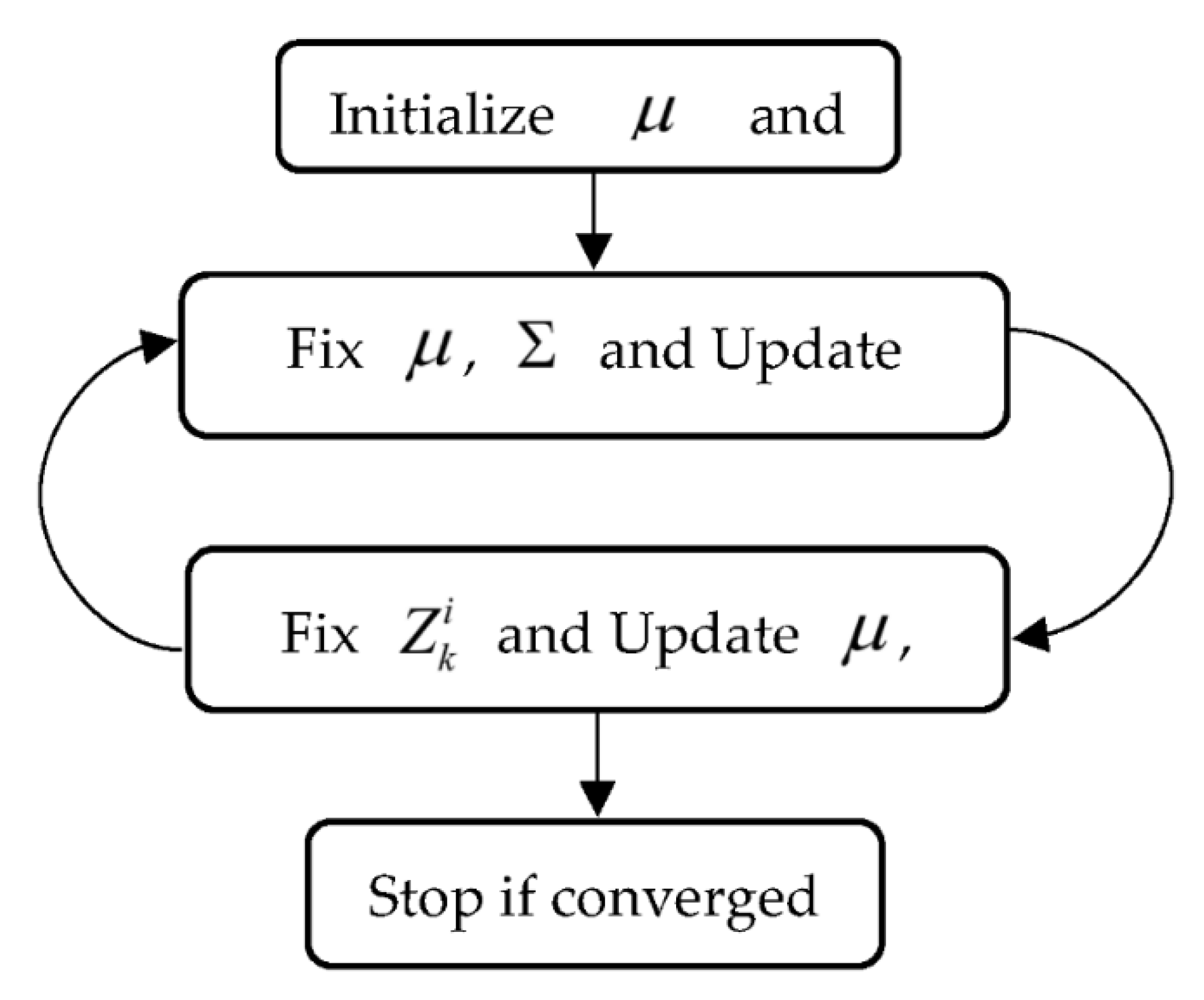
After the initial clustering of the original data using the ADPC algorithm is completed. The initial values $\zeta$ can be determined, and the EM algorithm is used to build the GMM. The implementation process is shown in Figure 6.

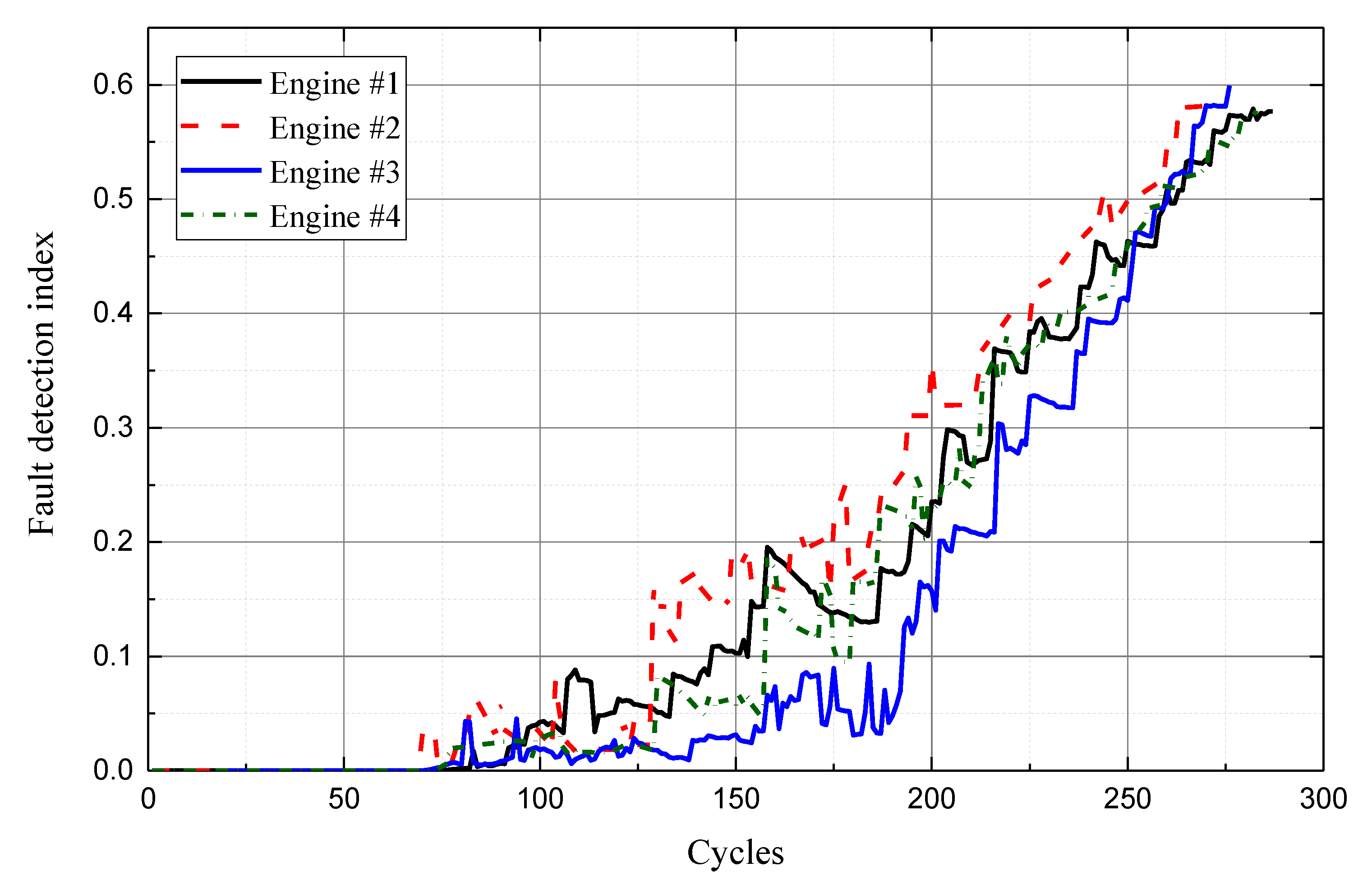
The GMM model for the health state and monitoring state need to be constructed. This kind of DP model is also called the dynamic double probability model. Among them, data from the top 25% of the engine life cycles is used to construct the baseline probability model, and this model remains unchanged in the process of engine fault diagnosis. Data from after 75% of the engine life cycles is used to construct the monitoring probability model, which is continuously updated with the increase of the engine life cycles. In the fault diagnosis stage, the most important thing is to get the engine fault detection indexes, as is shown in Figure 7. In the probability difference measuring method, the number of Monte Carlo samples is R = 10,000.

Table 2. Parameters related to the four engines.

Engine No.	Full Life Cycle	Fault Detection Index at the End of the Cycle
Engine #1	287	0.5768
Engine #2	269	0.5814
Engine #3	276	0.5885
Engine #4	283	0.5747

shows the relevant parameters of the four engines and the fault detection indexes in case of engine failure. It can be seen from the figure that the fault detection indexes of the top 25% cycles are zero. This is because the engine is in a healthy state at this stage and failure monitoring is not carried out. In the fault monitoring stage, the fault detection index’s variation trend of the four engines is basically the same. Since the initial value and total life cycles of each engine are slightly different (this is a characteristic of the C-MAPSS data set itself), the four curves do not completely coincide in the early stage, but they tend to coincide very well in the later stage. And all four engines have almost the same fault detection index at the end of the cycle. These results are quite consistent with the real failure evolution law of engine.

In order to verify the superiority of the proposed model, BP and DBN models are used as comparison, among which the BP model is a classic algorithm, whereas the DBN model is a new and effective method used for engine fault diagnosis in recent years. Figure 8 indicates the analysis results of five samples, which are also from the C-MAPSS data (The relevant data of BP and DBN models are from reference [1]). The results show that the fault detection indexes obtained by BP or DBN models oscillate violently.

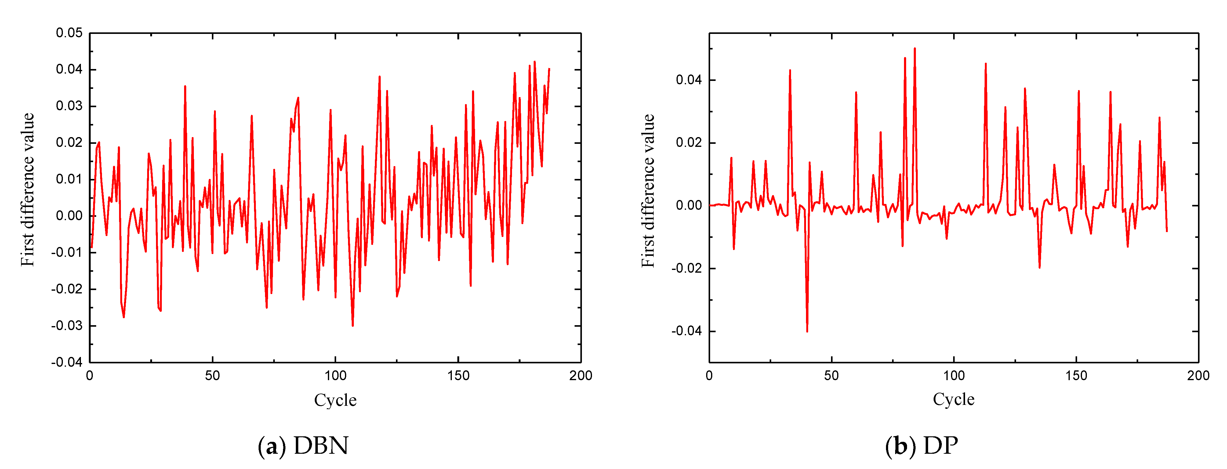
In order to compare the effect of the model more specifically, the first-order difference of the predicted fault detection indexes and the corresponding variance value are obtained, as shown in Figure 9. The variance of the proposed DP model is 0.015, whereas the variance of the BP and DBN models are 0.035 and 0.024, respectively, as shown in

Table 3. Comparison results of variance values of three models.

Model	Difference Variance (10−2)
BP	3.5
DBN	2.4
DP	1.5

. Obviously, the proposed DP model has lower difference variances and better fault diagnosis results compared with the BP model and DBN model. Unlike the DBN and other ANN methods, the key to the DP model is to construct the probability distribution of engine data set in a specific space, which is the statistical result of a large number of data. Therefore, the DP model has the ability to integrate historical data and current data, and its stability is bound to be better.

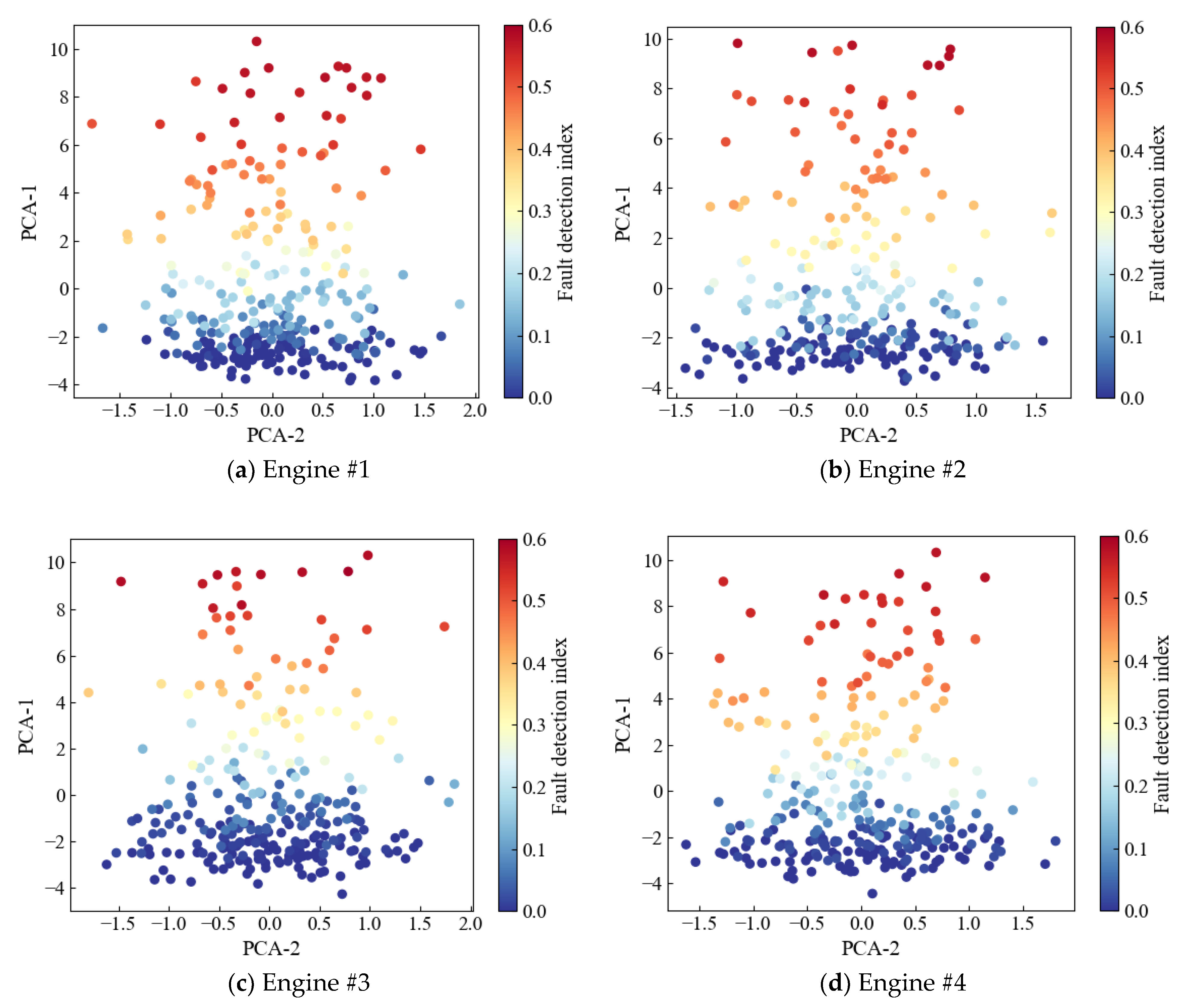
It is expected that the dynamic double probability model is able to capture the manifold of the healthy state and map differences between degradation trajectories into different regions of 2D FMF space. This visualization is given in Figure 10 using the first two principal components combined with the fault detection indexes. As can be seen from the figure, blue data points representing engine health status are mainly concentrated around PCA-1 = −3. As PCA-1 increases, the value of fault detection indexes also increases. The fault monitoring index reaches the maximum at about PCA-1 = 10 for all four engines, which means engine failure. It is clear that the DP model can well identify the evolution process of engine failure.

4.3. RUL Estimation

The DP + LSTM model is applied for RUL estimation. It is necessary to select appropriate parameters for LSTM models to avoid local optimum and fitting errors. As a matter of experience, the optimal parameter combinations of the LSTM model are shown in

Table 4. Designs based for LSTM networks.

Model Parameters	Value
Layer	3
Hidden units	[128, 64, 64]
Dropout	[0.3, 0.3, 0]
Batch size	100
Epoch	100
Input shape	[10, 1]
Output shape	[1, 1]

. The 80 representative engines in the C-MAPSS dataset are used to verify the reliability of the LSTM model, in which the training and test subsets are divided into a ratio of 3:1. The training data of LSTM is the fault detection indexes for each engine.

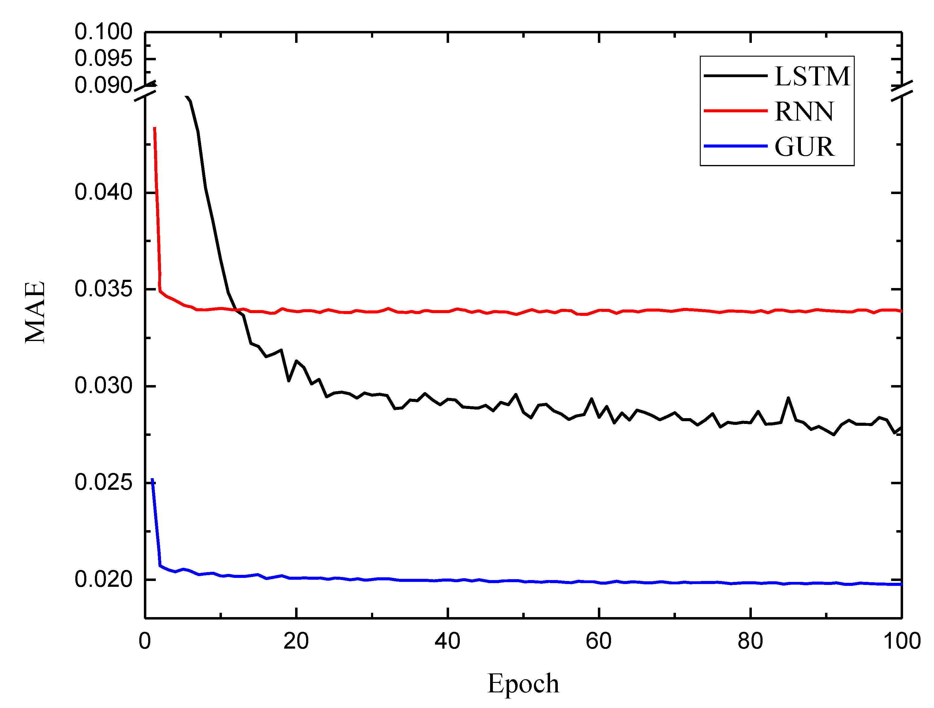
To verify the superiority of the proposed method, the RNN and gated recurrent unit (GRU) network, which is a variant of LSTM, are implemented as comparisons [1], Mean absolute error (MAE) is used as a training loss function, and the MAE values of the three models are shown in Figure 11. The results show that the training loss of these three models decreases gradually with the increasing epoch. When the epoch reaches 100, the training loss of LSTM is lower than that of RNN but higher than that of GRU. During the last 20 epochs, the mean loss is 0.028.

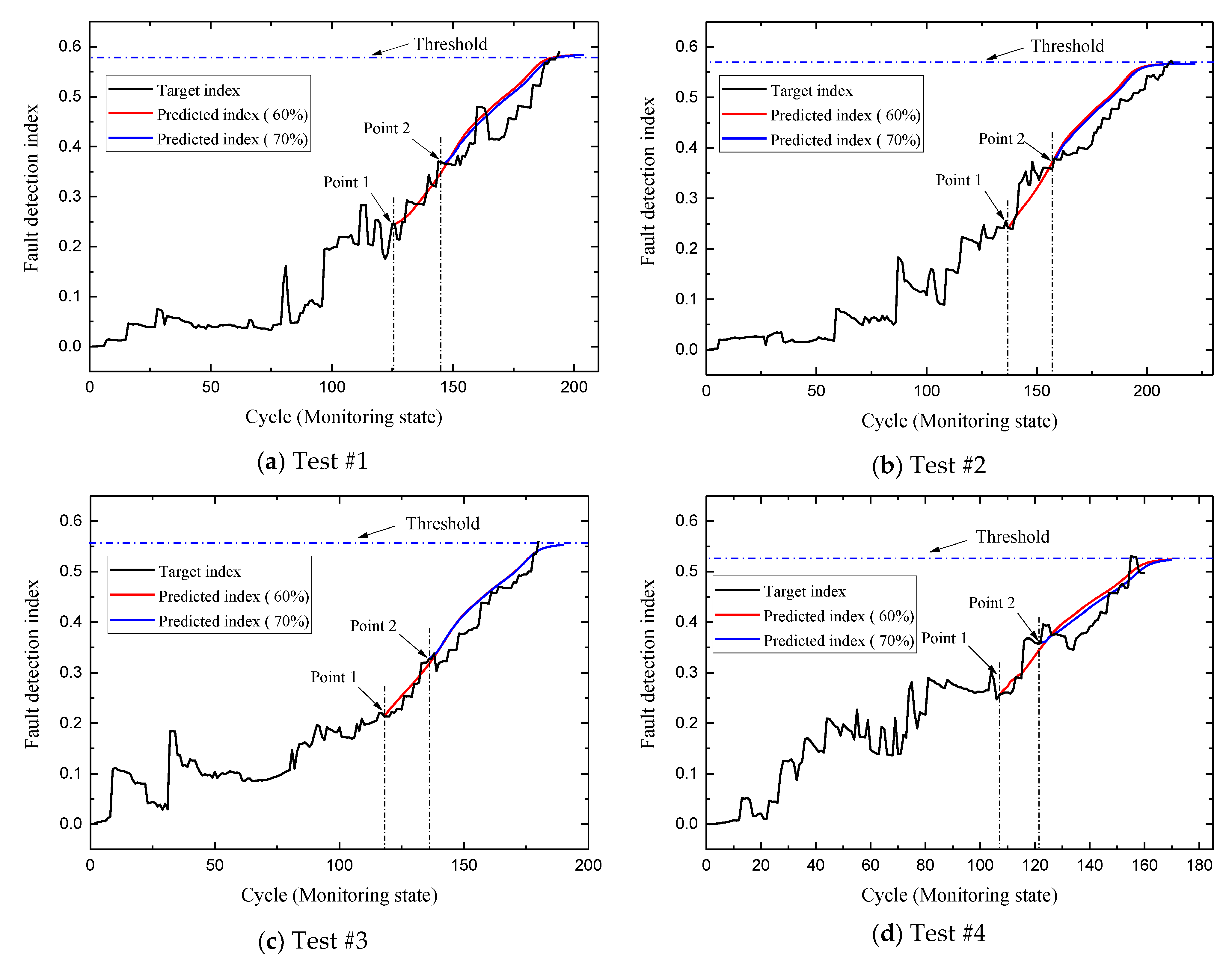
Figure 12 plots the prediction result of four testing sets from 60% and 70% of the monitoring cycles. As can be seen from the figure, the predicted results are in good agreement with the actual results. Especially near the cycle of engine failure, the actual value is highly coincident with the predicted value. High precision prediction can be achieved whether the prediction starts from 60% or 70% of the monitoring period. LSTM is a time series prediction model, and the prediction ability it has learned does not include the prediction after engine failure. Therefore, when the prediction curve tends to be stable, it means that the engine is about to fail. In addition, the prediction curve flattens out after the failure point and shows little growth. These prove the reliability and accuracy of the DP model and LSTM model proposed in this paper. The threshold needs to be set for RUL estimation since the initial state of each engine in the C-MAPSS data set is different, and the threshold value will vary slightly. The threshold value of the four engines selected in Figure 12 can be set to about 0.55.

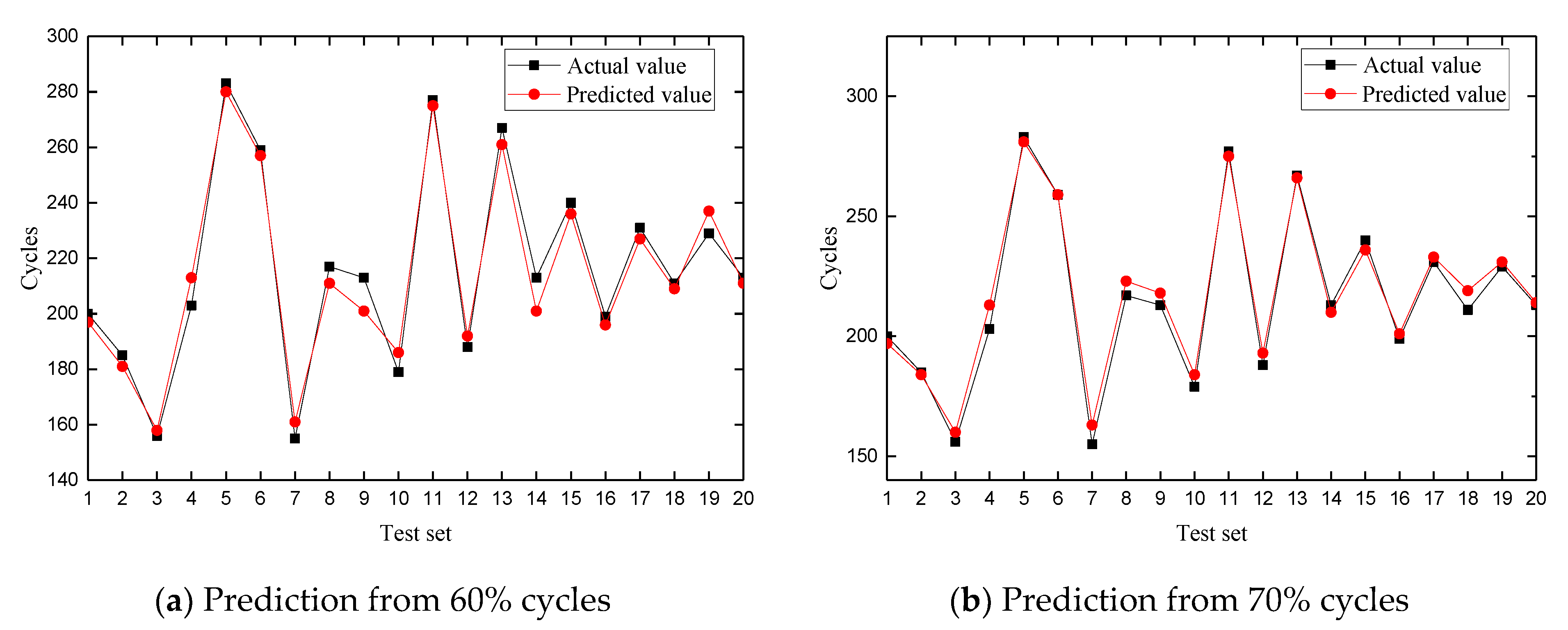
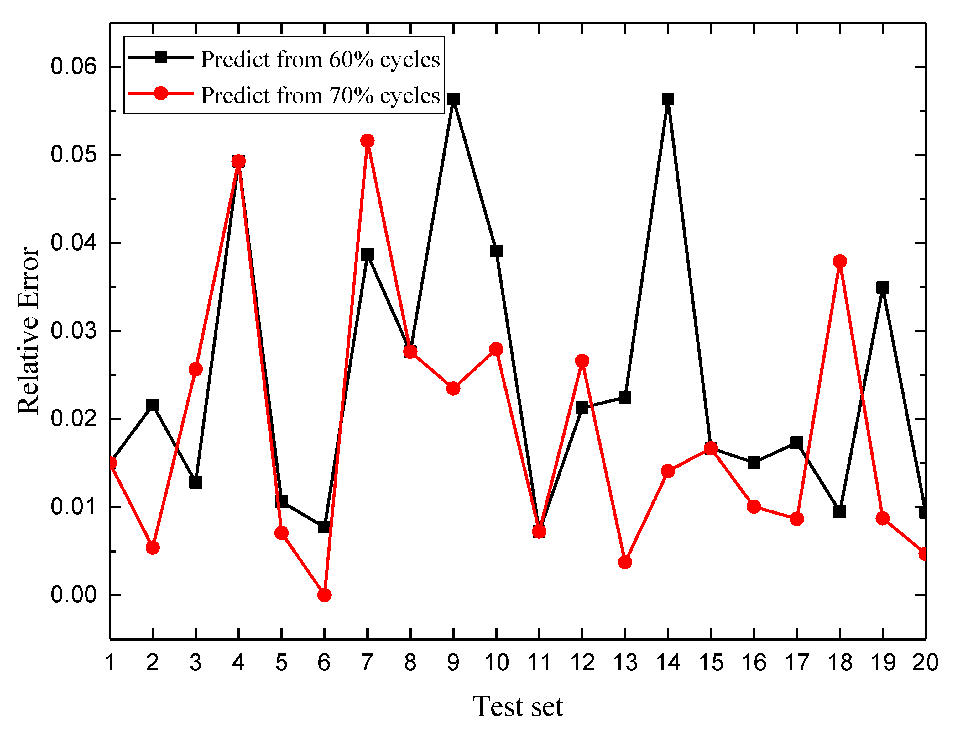
The engine cycles corresponding to the threshold can be determined according to the prediction curve; that is, the cycle when the failure is predicted. To get a more detailed understanding of the model’s accuracy, we calculated the relative error of prediction for 20 testing sets, as shown in Figure 13 and Figure 14. When predicted from 60% cycles, the mean relative error of the testing is 0.024%. When predicted from 70% cycles, the mean relative error of the testing is 0.019%. Obviously, the prediction accuracy is slightly higher when starting from 70% cycles, because time series prediction models generally have a certain degree of cumulative error. In general, the relative errors of both of them remain below 6%, which proves the high accuracy of the proposed model.

Several classical RUL estimation methods are compared to verify the superiority of the proposed method, and the RUL prediction errors of the five models are listed in

Table 5. RUL estimation error of different models.

Model	Point 1 (Cycles)	Point 2 (Cycles)	Average (Cycles)
DP + LSTM	5.1	3.7	4.4
DBN + LSTM	6.9	4.4	5.6
LSTM	8.2	6.8	7.5
RNN	10.2	7.9	9.0
GRU	10.0	7.0	8.5

(relevant data of the model used for comparison come from the reference [1]). Compared with DBN + LSTM, LSTM, RNN, and GRU, the average RUL estimation error of DP + LSTM model is 4.4, which decreases by 21%, 41%, 51%, and 48% (the data of these five models are all from the C-MAPSS dataset). The result shows that proposed DP + LSTM model has higher accuracy than those classical time series prediction models. In fact, several other methods belong to the ANN model, which can also be called a black box model. In essence, they achieve prediction by learning the inherent laws of a large amount of data. These methods are sensitive to data, and the hyper-parameters have a great impact on the model effect, and the adjustment of hyper-parameters is a complex process. The DP + LSTM method proposed in this study is the combination of probability model and ANN model. Solid mathematical basis is the advantage of probability model, which is an important factor for the DP + LSTM model to be more superior.

4.4. PHM Application Example

Standardizing the data processing flow of the PHM framework is one of the aims of this study. Algorithm 1 summarizes the function realization process of the PHM framework.

Algorithm 1. PHM framework process.

Input: Aero-engine raw sensor data. Process 1: Data preprocessing     (1) Data collation and standardization (z-score).     (2) Data dimension reduction based on PCA method. Process 2: DP model construction     (1) The preprocessed data are fed to the double probability models.     (2) Construct the baseline probability model.     (3) Construct the dynamic monitoring probability model.     (4) Difference measures for double probability models.     (5) Output fault detection indexes. Process 3: RUL Estimation     (1) Training LSTM network based on fault detection indexes.     (2) The prediction of engine RUL at the current time is realized from any cycle point in the engine life cycle.     (3) Output engine RUL. Output: Fault detection indexes and RUL.

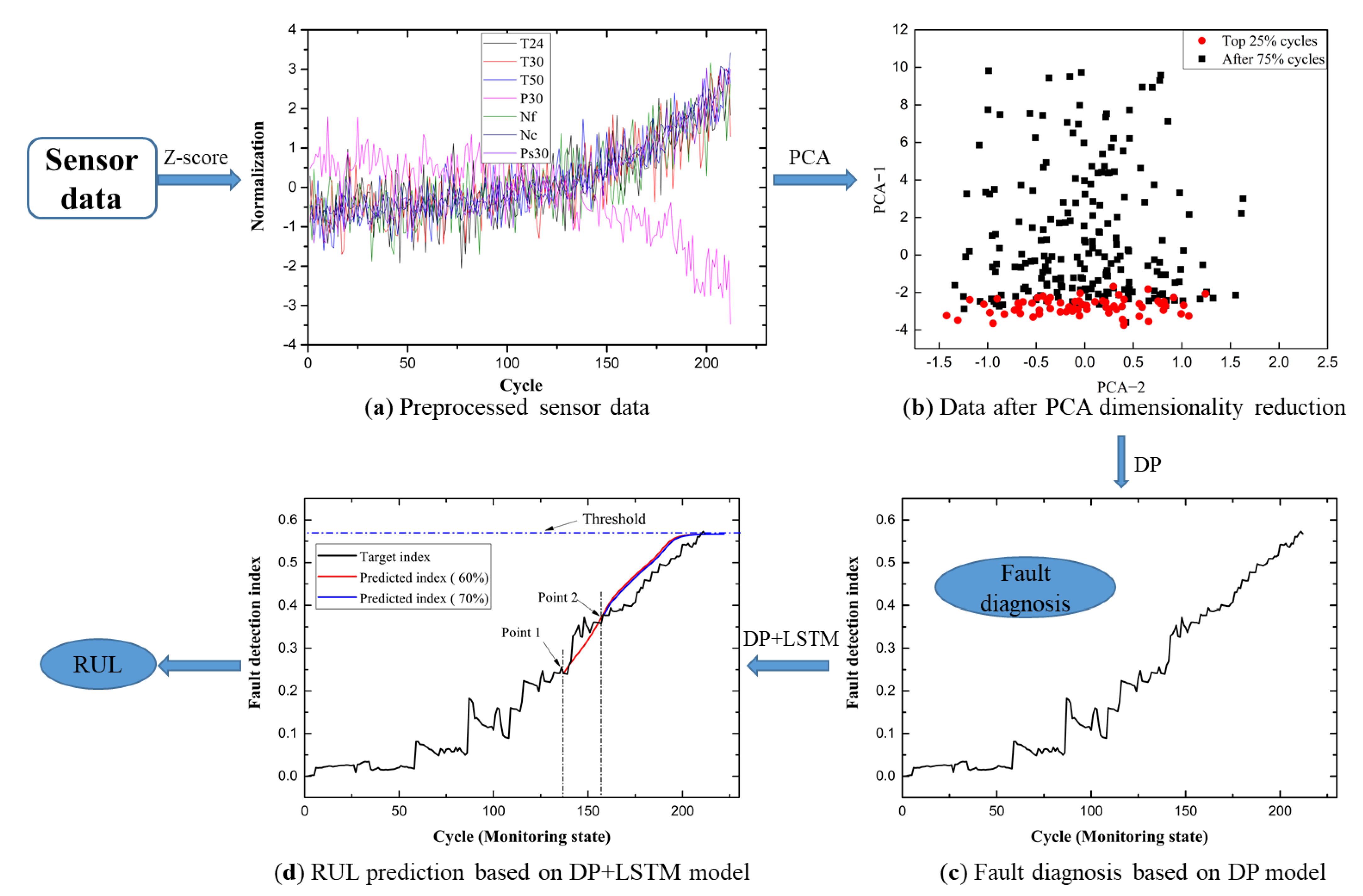
An engine data set in the C-MAPSS data set is selected to show the processing results of the proposed PHM framework, as shown in Figure 15a, which shows 7 of the 14 sets of raw sensor data for the engine. It can be seen that noise greatly interferes with sensor data, and the change trends of sensors are inconsistent in the whole life cycle of the engine. Figure 15b shows the data after dimension reduction. Figure 15c,d, respectively, show the results of fault diagnosis and RUL estimation respectively. The proposed framework realizes data analysis and mining from the original data of the engine to monitor engine health and realize the estimation of RUL.

5. Conclusions

In this study, a PHM framework combining the DP model and LSTM model is proposed for fault diagnosis and RUL estimation of aero-engine. Firstly, the DP model consisting of a baseline probability model and a monitoring probability model is constructed, in which the baseline probability model reflects the operating characteristics of the engine’s healthy state, and the monitoring probability model reflects the failure occurrence and evolution process of the engine. A GMM-ADPC algorithm is employed for modeling engine fault development, and the PCA method is adopted to reduce the dimension of the input data. Secondly, the probability difference measuring method is used to quantify the difference between the two probability models so as to obtain the fault detection indexes. Thirdly, the DP + LSTM model is introduced for a time series prediction of fault detection indexes, so as to estimate the RUL of the engine. Finally, the PHM framework is established by integrating the aforementioned models. The experimental results on the degradation datasets obtained by the C-MAPSS indicated that the proposed DP model can capture the process of engine failure well, and the DP + LSTM model can perform RUL estimation well. By comparing the results of the proposed method with some classical methods, it is shown that the proposed method has better stability and accuracy.

To sum up, the PHM framework proposed in this study can adequately realize the functions of fault diagnosis and RUL estimation.

References

1. Che, C.; Wang, H.; Fu, Q.; Ni, X. Combining multiple deep learning algorithms for prognostic and health management of aircraft. Aerosp. Sci. Technol. 2019, 94, 105423. [Google Scholar] [CrossRef]
2. Huang, Y.; Sun, G.; Tao, J.; Hu, Y.; Yuan, L. A modified fusion model-based/data-driven model for sensor fault diagnosis and performance degradation estimation of aero-engine. Meas. Sci. Technol. 2022, 33, 085105. [Google Scholar] [CrossRef]
3. Cui, L.; Zhang, C.; Zhang, Q.; Wang, J.; Wang, Y.; Shi, Y.; Lin, C.; Jin, Y. A Method for Aero-Engine Gas Path Anomaly Detection Based on Markov Transition Field and Multi-Lstm. Aerospace 2021, 8, 374. [Google Scholar] [CrossRef]
4. Tolani, D.; Yasar, M.; Chin, S.; Ray, A. Anomaly detection for health management of aircraft gas turbine engines. In Proceedings of the 2005 American Control Conference, Portland, OR, USA, 8–10 June 2005; pp. 459–464. [Google Scholar]
5. Fornlöf, V.; Galar, D.; Syberfeldt, A.; Almgren, T. RUL estimation and maintenance optimization for aircraft engines: A system of system approach. Int. J. Syst. Assur. Eng. Manag. 2016, 7, 450–461. [Google Scholar] [CrossRef]
6. Lu, S.; Zhou, W.; Huang, J.; Lu, F.; Chen, Z. A Novel Performance Adaptation and Diagnostic Method for Aero-Engines Based on the Aerothermodynamic Inverse Model. Aerospace 2022, 9, 16. [Google Scholar] [CrossRef]
7. Yan, L.; Zhang, H.; Dong, X.; Zhou, Q.; Chen, H.; Tan, C. Unscented Kalman-filter-based simultaneous diagnostic scheme for gas-turbine gas path and sensor faults. Meas. Sci. Technol. 2021, 9, 49. [Google Scholar] [CrossRef]
8. Baumann, M.; Koch, C.; Staudacher, S. Application of Neural Networks and Transfer Learning to Turbomachinery Heat Transfer. Aerospace 2022, 9, 49. [Google Scholar] [CrossRef]
9. Zaccaria, V.; Fentaye, A.D.; Stenfelt, M.; Kyprianidis, K.G. Probabilistic Model for Aero-Engines Fleet Condition Monitoring. Aerospace 2020, 7, 66. [Google Scholar] [CrossRef]
10. El-Thalji, I.; Jantunen, E. A summary of fault modelling and predictive health monitoring of rolling element bearings. Mech. Syst. Signal Process. 2015, 60, 252–272. [Google Scholar] [CrossRef]
11. Lu, F.; Wu, J.; Huang, J.; Qiu, X. Aircraft engine degradation prognostics based on logistic regression and novel OS-ELM algorithm. Aerosp. Sci. Technol. 2019, 84, 661–671. [Google Scholar] [CrossRef]
12. Ochella, S.; Shafiee, M.; Sansom, C. Adopting machine learning and condition monitoring P-F curves in determining and prioritizing high-value assets for life extension. Expert Syst. Appl. 2021, 176, 114897. [Google Scholar] [CrossRef]
13. Zhao, Y.P.; Song, F.Q.; Pan, Y.T.; Li, B. Retargeting extreme learning machines for classification and their applications to fault diagnosis of aircraft engine. Aerosp. Sci. Technol. 2017, 71, 603–618. [Google Scholar] [CrossRef]
14. Fentaye, A.D.; Ul-Haq Gilani, S.I.; Baheta, A.T.; Li, Y.G. Performance-based fault diagnosis of a gas turbine engine using an integrated support vector machine and artificial neural network method. Proc. Inst. Mech. Eng. Part A J. Power Energy 2019, 233, 786–802. [Google Scholar] [CrossRef]
15. Li, Y.; Du, X.; Wan, F.; Wang, X.; Yu, H. Rotating machinery fault diagnosis based on convolutional neural network and infrared thermal imaging. Chin. J. Aeronaut. 2020, 33, 427–438. [Google Scholar] [CrossRef]
16. Soualhi, A.; Clerc, G.; Razik, H.; Guillet, F. Hidden Markov Models for the Prediction of Impending Faults. IEEE Trans. Ind. Electron. 2016, 63, 3271–3281. [Google Scholar] [CrossRef]
17. Lambert, P.; Eilers, P.H. Bayesian proportional hazards model with time-varying regression coefficients: A penalized Poisson regression approach. Stat. Med. 2005, 24, 3977–3989. [Google Scholar] [CrossRef]
18. Ochella, S.; Shafiee, M.; Dinmohanmmadi, F. Artificial intelligence in prognostics and health management of engineering systems. Eng. Appl. Artif. Intel. 2022, 108, 104552. [Google Scholar] [CrossRef]
19. Sohn, H. Effects of environmental and operational variability on structural health monitoring. Philos. Trans. A Math. Phys. Eng. Sci. 2007, 365, 539–560. [Google Scholar] [CrossRef]
20. Gao, D.; Wu, Z.; Yang, L.; Zheng, Y.; Yin, W. Structural health monitoring for long-term aircraft storage tanks under cryogenic temperature. Aerosp. Sci. Technol. 2019, 92, 881–891. [Google Scholar] [CrossRef]
21. Qiu, L.; Fang, F.; Yuan, S.; Boller, C.; Ren, Y. An enhanced dynamic Gaussian mixture model–based damage monitoring method of aircraft structures under environmental and operational conditions. Struct. Health Monit. 2019, 18, 524–545. [Google Scholar] [CrossRef]
22. Fang, F.; Qiu, L.; Yuan, S.; Ren, Y. Dynamic probability modeling-based aircraft structural health monitoring framework under time-varying conditions: Validation in an in-flight test simulated on ground. Aerosp. Sci. Technol. 2019, 95, 105467. [Google Scholar] [CrossRef]
23. Aydemir, H.; Zengin, U.; Durak, U. The digital twin paradigm for aircraft—Review and outlook. In Proceedings of the AIAA Scitech 2020 Forum, Orlando, FL, USA, 6–10 January 2020; pp. 1–12. [Google Scholar]
24. Pernkopf, F.; Bouchaffra, D. Genetic-based EM algorithm for learning Gaussian mixture models. IEEE Trans. Pattern Anal. Mach. Intell. 2005, 27, 1344–1348. [Google Scholar] [CrossRef] [PubMed]
25. Soualhi, A.; Medjaher, K.; Zerhouni, N. Bearing Health Monitoring Based on Hilbert–Huang Transform, Support Vector Machine, and Regression. IEEE Trans. Instrum. Meas. 2015, 64, 52–62. [Google Scholar] [CrossRef]
26. Li, J.; Jing, B.; Dai, H.; Sheng, Z.; Jiao, X.; Liu, X. A remaining useful life prediction method for airborne fuel pump after maintenance. Proc. Inst. Mech. Eng. Part. G J. Aerosp. Eng. 2019, 233, 5660–5673. [Google Scholar] [CrossRef]
27. Listou Ellefsen, A.; Bjørlykhaug, E.; Æsøy, V.; Ushakov, S.; Zhang, H. Remaining useful life predictions for turbofan engine degradation using semi-supervised deep architecture. Reliab. Eng. Syst. Safe. 2019, 183, 240–251. [Google Scholar] [CrossRef]
28. Li, R.; Verhagen, W.J.C.; Curran, R. Toward a methodology of requirements definition for prognostics and health management system to support aircraft predictive maintenance. Aerosp. Sci. Technol. 2020, 102, 105877. [Google Scholar] [CrossRef]
29. Figueiredo Mario, A.T.; Jain Anil, K. Unsupervised learning of finite mixture models. IEEE Trans. Pattern Anal. Mach. Intell. 2002, 24, 381–396. [Google Scholar] [CrossRef]
30. Chakraborty, D.; Kovvali, N.; Papandreou-Suppappola, A.; Chattopadhyay, A. An adaptive learning damage estimation method for structural health monitoring. J. Intell. Mater. Syst. Struct. 2015, 26, 125–143. [Google Scholar] [CrossRef]
31. Yang, Z.; Wang, H.; Zhou, Y. A Clustering Algorithm with Adaptive Cut-off Distance and Cluster Centers. Data Anal. Knowl. Discov. 2018, 3, 39–48. (In Chinese) [Google Scholar]
32. Rodriguez, A.; Laio, A. Clustering by fast search and find of density peaks. Science 2014, 344, 1492–1496. [Google Scholar] [CrossRef]
33. Van Erven, T.; Harremos, P. Rényi divergence and kullback-leibler divergence. IEEE Trans. Inf. Theory 2014, 60, 3797–3820. [Google Scholar] [CrossRef]
34. Leser Patrick, E.; Warner James, E.; Leser William, P.; Bomarito Geoffrey, F.; Newman John, A.; Hochhalter Jacob, D. A digital twin feasibility study (Part II): Non-deterministic predictions of fatigue life using in-situ diagnostics and prognostics. Eng. Fract. Mech. 2020, 229, 106903. [Google Scholar] [CrossRef]
35. Bengio, Y.; Simard, P.; Frasconi, P. Learning Long-Term Dependencies with Gradient Descent is Difficult. IEEE Trans. Neural Netw. 1994, 5, 157–166. [Google Scholar] [CrossRef] [PubMed]
36. Hochreiter, S.; Schmidhuber, J. Long short-term memory. Neural Comput. 1997, 9, 1735–1780. [Google Scholar] [CrossRef] [PubMed]
37. Guo, L.; Li, N.; Jia, F.; Lei, Y.; Lin, J. A recurrent neural network based health indicator for remaining useful life prediction of bearings. Neurocomputing 2017, 240, 98–109. [Google Scholar] [CrossRef]
38. Zhang, J.; Wang, P.; Yan, R.; Gao, R.X. Long short-term memory for machine remaining life prediction. J. Manuf. Syst. 2018, 48, 78–86. [Google Scholar] [CrossRef]
39. Badea, V.E.; Zamfiroiu, A.; Boncea, R. Big Data in the Aerospace Industry. Inform. Econ. 2018, 22, 17–24. [Google Scholar] [CrossRef]
40. Li, C.; Mahadevan, S.; Ling, Y.; Choze, S.; Wang, L. Dynamic Bayesian network for aircraft wing health monitoring digital twin. AIAA J. 2017, 55, 930–941. [Google Scholar] [CrossRef]
41. Lu, C.; Wang, S.; Makis, V. Fault severity recognition of aviation piston pump based on feature extraction of EEMD paving and optimized support vector regression model. Aerosp. Sci. Technol. 2017, 67, 105–117. [Google Scholar] [CrossRef]
42. Saxena, A.; Goebel, K.; Simon, D.; Eklund, N. Damage propagation modeling for aircraft engine run-to-failure simulation. In Proceedings of the 2008 IEEE International Conference on Prognostics and Health Management, Denver, CO, USA, 6–9 October 2008; pp. 1–9. [Google Scholar]
43. Vollert, S.; Theissler, A. Challenges of machine learning-based RUL prognosis: A review on NASA’s C-MAPSS data set. In Proceedings of the 2021 26th IEEE International Conference on Emerging Technologies and Factory Automation (ETFA), Vasteras, Sweden, 7–10 September 2021; pp. 1–8. [Google Scholar]
44. Li, L.; Shi, W. A fault tolerant model for multi-sensor measurement. Chin. J. Aeronaut. 2015, 28, 874–882. [Google Scholar] [CrossRef]
Figure 1. Building block of long short-term memory (LSTM) network [1].
Aerospace 09 00316 g001
Figure 2. DP-LSTM modeling-based aero-engine PHM Framework.
Aerospace 09 00316 g002
Figure 3. Diagram of engine in C-MAPSS.
Aerospace 09 00316 g003
Figure 4. Two-dimensional PCA plot of the four engines.
Aerospace 09 00316 g004
Figure 5. The number of GCs along with the engine life cycle.
Aerospace 09 00316 g005
Figure 6. Steps of E-M algorithm.
Aerospace 09 00316 g006
Figure 7. Failure monitoring results in C-MAPSS data.
Aerospace 09 00316 g007
Figure 8. Comparison of BP and DBN for fault diagnosis of several samples [1].
Aerospace 09 00316 g008
Figure 9. First difference value of the fault detection indexes.
Aerospace 09 00316 g009
Figure 10. Two-dimensional PCA plot of the fault detection index.
Aerospace 09 00316 g010
Figure 11. The loss contrast among LSTM, GRU, and RNN.
Aerospace 09 00316 g011
Figure 12. RUL prediction of 4 engines.
Aerospace 09 00316 g012
Figure 13. The residuals of the actual RUL and estimated RUL on 20 testing sets.
Aerospace 09 00316 g013
Figure 14. The relative error of RUL prediction on 20 testing sets.
Aerospace 09 00316 g014
Figure 15. Example of PHM framework data processing flow.
Aerospace 09 00316 g015