A Generic Mission-Level Flight Control Surface EMA Power Consumption Simulation Tool

Abstract

The use of electromechanical actuators (EMAs) for aeronautical applications promises substantial benefits regarding efficiency and operability. To advance the design of power electronics and secondary power supply, there is a need for the ability to swiftly study the effects of aircraft mission and operational aspects on the actuator energy consumption. Pursuant to this, the aim of the work presented in this paper is twofold: (i) to build a generic mission-level flight control surface EMA power consumption simulation framework and (ii) to apply this framework to a case study involving a small all-electric aircraft, in which selected factors that impact energy consumption are investigated. The core of the framework comprises physics-based EMA power estimators, linked with a six-degree-of-freedom flight dynamics and control simulation module. The case study results show that the actuator power consumption correlates positively with the proportional gains in the flight control system but is inversely proportional to the trajectory radius and linearly dependent on turbulence intensity. The developed framework could aid in the selection of the actuator, as well as in the optimisation of airborne electronics and secondary power supply.

1. Introduction

For aeronautical applications, electromechanical actuators (EMAs) can offer several advantages over more traditional hydraulic actuators. These advantages relate to efficiency, operability, and maintainability, as employing EMAs can enable comparatively complicated and heavy centralised hydraulic systems to be eliminated. The study of the design and architecture analysis of these actuators is therefore becoming more widespread, and the body of literature is growing [1,2,3].

One area of active research involves the development of modelling and simulation tools to study and predict actuator energy consumption for different systems, mission trajectory, and flight condition factors [4,5]. Such tools are particularly essential to electric aircraft design, as the actuator energy consumption sizing, which affects power management optimization and secondary power supply sizing, can significantly impact flight endurance [6,7]. Examples of these include micro aerial vehicles, high altitude long endurance (HALE) aircraft, and more exotic aircraft, such as solar-powered aircraft, where atmospheric turbulence can significantly affect actuator power consumption [8,9].

Our previous work focused on producing a mission-level EMA energy consumption simulation framework [4]. Although enabling studying the aircraft-level energy consumption characteristics of the actuators, this framework has several limitations. These include limitations due to simplified modelling of the EMAs, the use of empirical methods for the prediction of control surface hinge moments (which limits the types of aircraft configurations that can be studied), and incomplete testing. Addressing these limitations would lead to a more generic and flexible tool that would enable more types of design and simulation studies to be performed on more types of aircraft.

The aim of the work presented in this paper was twofold: (i) to establish a generic flight control surface EMA energy consumption simulation framework and (ii) to demonstrate its capabilities by employing it to investigate selected factors that would affect EMA energy consumption.

To achieve this aim, the framework had to include a six-degree-of-freedom (6DOF) flight dynamics and control module, a new, more generic aerodynamics and hinge moment prediction module, and an actuator power ‘estimator’ in which more of the relevant physics is modelled.

In relation to the first part of the aim, the development of this framework is discussed in detail in this paper. The framework was developed in MATLAB Simulink^®, as this environment is highly suited to the time-based simulation of complex systems. Furthermore, addressing the second part of the aim, the application of the framework to a case study involving an investigation of the effects of turbulence intensity, proportional gains in the flight control algorithm, and aircraft trajectory radius on actuator energy consumption in a waypoint fly-over mission is also presented.

This introduction is followed by a short overview of previous related research. In Section 3, the framework architecture is introduced, followed in Section 4 by the case study. Finally, the paper is concluded, and future work is presented in Section 5.

2. Overview of Previous Related Research

Apart from work on improving the basic underlying technology, there is an increasing focus in the literature on studying and advancing the aircraft-level energy consumption characteristics of systems involving EMAs [4,5]. Swift, accurate prediction of actuator energy-use for the whole flight envelope can provide significant support in the design or selection of actuators, as well as the sizing of secondary power systems.

Several previous efforts involved studies related to actuator energy consumption in flight. In Ref. [5], the electric consumption of different actuator configurations was analysed for a single flight profile. The electricity drawn from the power buses was determined by control surface deflection angular velocities and hinge moments (as determined by an empirical method), as well as component efficiencies and gear ratios. The average surface actuation energy consumption was then calculated for each separate flight segment, using the mean predicted power for when the actuators are active. The implementation of the trajectory analysis and mean power calculations enable the evaluation of actuator system energy consumption; however, for small aircraft, such as UAVs, aerodynamic results from the empirical methods may require a corrective curve for low Reynolds numbers [10]. In Ref. [11], Simpson pointed out that the hinge moment result from DATCOM (a commonly used tool for predicting stability and control of air vehicles) does not include the term $\partial C_{h\delta }/\partial \alpha$, and therefore cannot represent a wide range of conditions. Furthermore, such steady-state methods may lack accuracy when transient effects are to be considered and therefore have limited flexibility when analysing the impact of several factors in flight.

The 6DOF flight simulation could be a powerful method to investigate flight control actuator energy consumption. In Ref. [12], the energy consumption requirement of three types of actuators, including EMAs, were analysed quantitatively as the application aircraft under consideration followed predefined trajectories under two multiple-input–multiple-output (MIMO) flight control schemes, total energy control system, and total heading control system (TECS/THCS). In Ref. [4], 6DOF simulation was also employed in a dynamic actuator power consumption tool for trajectory optimization. In that study, the EMA power models interacted with the control surface load estimator to obtain the transient power during different flight segments. However, the model was limited in several respects. For example, the EMA modelling was simplified considerably, with electrical and magnetic losses merely represented by an ‘equivalent resistance’. This resistance was ‘selected’ such as to make the efficiency equal to 30%. Furthermore, the aerodynamic modelling was performed based on the data of a small UAV and is therefore specific to that aircraft.

For some unconventional aircraft configurations, empirical methods for hinge moment estimation may lack flexibility and accuracy. The use of Vortex-Lattice Methods (VLM) for aerodynamics estimation has shown promise for modelling novel unconventional configurations [13,14]. Under the assumption of all potential flow (incompressible, inviscid, and irrotational), thin lifting surface, and small angle approximation, VLM is valid for estimating hinge moments with reasonable accuracy in certain cases, where the control surface deflections and the angle of attack and sideslip are both small (usually less than 15° [11,15]). Care should also be taken for cases where the Reynolds numbers are small, as viscid effects may negate the inviscid assumption for VLM (the lift and hinge moment result under full potential flow assumption can be fairly accurate for the Reynolds number regime from 8.4 × 10⁴ to 4.2 × 10⁵ [10]). If adhering to these constraints, VLM can be a powerful tool to study hinge moment characteristics for a wide range of aircraft [11,16]. It was, therefore, a goal of this study to incorporate a VLM aerodynamics solver into the proposed framework.

From this literature survey, it was concluded that to analyse the EMA power characteristics at the aircraft level, 6DOF flight simulation can be the most advantageous approach; however, improved EMA modelling (especially electromagnetic modelling) can support the accuracy of electric consumption estimation. Furthermore, to devise a truly generic framework, by enabling more types of configurations to be studied, the use of VLM for hinge moment estimation should be investigated further.

3. Proposed Simulation Framework

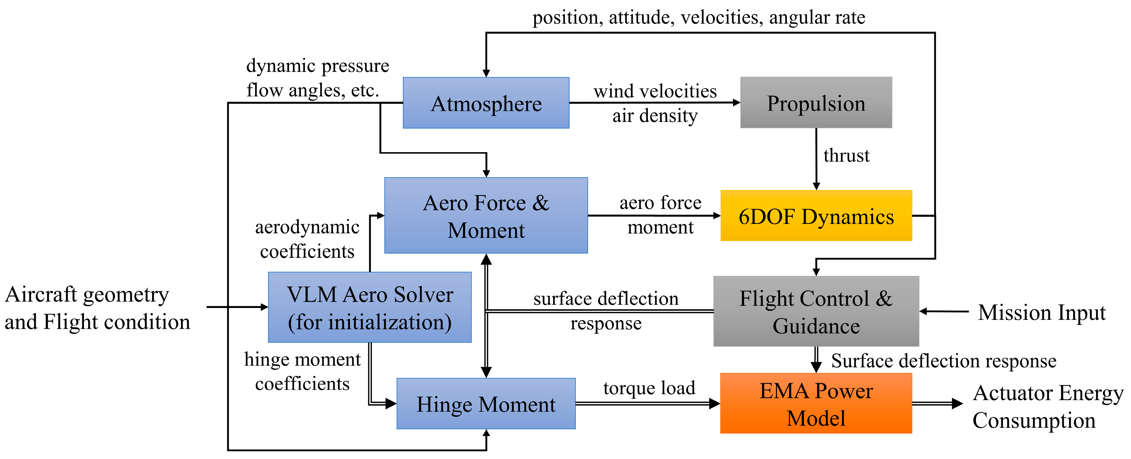
In this section, the framework architecture and main functional modules are described. These are represented by the top-level block diagram in Figure 1. The modularity of the framework is based on a rigid interface definition between blocks, which simplifies the substitution of individual modules for different aircraft or flight missions.

Figure 1. Block diagram representing the simulation framework.

There are eight top-level modules, divided into four types: ‘Atmosphere and Aerodynamics (blue)’, ‘Control Input (grey)’, ‘EMA Power Estimator (orange)’, and ‘6DOF Dynamics (yellow)’. To initialize the simulation, the ‘VLM Aero Solver’ calculates and exports the aerodynamics and hinge moment coefficients to be used by the ‘Aero Force and Moment’ and ‘Hinge Moment’ modules. During the simulation, the ‘6DOF Dynamics’ module updates the flight parameter vectors, such as position, attitude, velocities, and angular rates. The ‘Atmosphere’ module computes wind velocities, density, and flow angles. The ‘Hinge Moment’ module updates the current torque load, which along with the surface deflection response, are processed in the ‘EMA Power Model’, resulting in a transient power consumption output.

Each of the blocks is introduced in more detail in the subsequent sections.

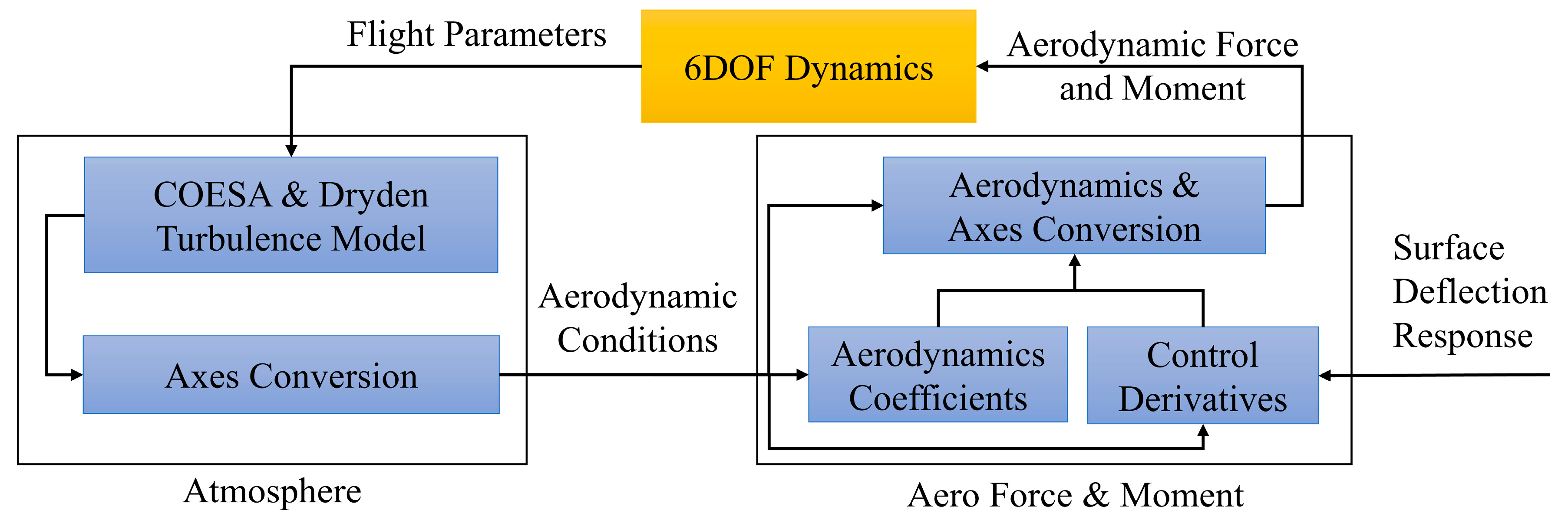
3.1. Atmosphere and Aero Force and Moment

The interaction between these two modules is shown in Figure 2.

Figure 2. The interaction between the Atmosphere and Aero Force and Moment modules.

Within the ‘Atmosphere’ module, the standard atmosphere model, which implements the mathematical representation of the 1976 Committee on Extension to the Standard Atmosphere (COESA) [17], calculates the atmospheric properties. Meanwhile, the Dryden turbulence model uses these parameters to determine transient turbulence properties, including angular and linear wind velocity [18]. These two models are standard blocks provided in the Aerospace toolbox within the MATLAB/Simulink Library. The atmospheric and turbulence properties are then transformed to aerodynamic conditions (wind velocity, angles of attack, and sideslip) with the ‘Axes Conversion’ block.

The ‘Aero Force and Moment’ block contains ‘Aerodynamic Coefficients’ and ‘Control Derivatives’ blocks, which generate corresponding data based on the aerodynamic conditions. The two blocks use a series of 2-D lookup tables, with indices of angles of attack and sideslip. These data are then sent to the ‘Aerodynamics & Axes Conversion’ block for the aerodynamic force and moment calculation and axes conversion (for conversion between wind axes and body axes).

The proposed aerodynamics framework was designed to simulate realistic atmospheric flight conditions, but two limitations still exist. The first is that the aircraft is modelled as rigid and the effects of aeroelasticity are therefore not taken into consideration. The second limitation is that the aerodynamic results from the VLM solver are only reliable in linear regions of the coefficient-parameter relationships (small deflections, large Reynolds numbers, and small angles of attack). Considering this simulation tool is established to address mission-level EMA power consumption for aircraft design, the rigid assumption and the linear combination of aerodynamic coefficients and control derivatives were deemed acceptable.

3.2. Hinge Moment

The ‘Hinge Moment’ module was built to generate the transient hinge moment during the flight simulation. The hinge moment derivatives for each control surface were stored in a series of 2-D lookup tables to which the inputs were angle of attack (angle of sideslip for rudder) and control surface deflection angle. The hinge moments on each surface at different aerodynamics conditions could be calculated with Equation (1). The atmospheric property is embodied in air density $\rho$.

$$T_{HM}={C_{HM}|}_{\alpha ,\delta }\overline{q}{A}_{w}c ,\overline{q}=\frac{1}{2}\rho {\overline{V}}^2$$

(1)

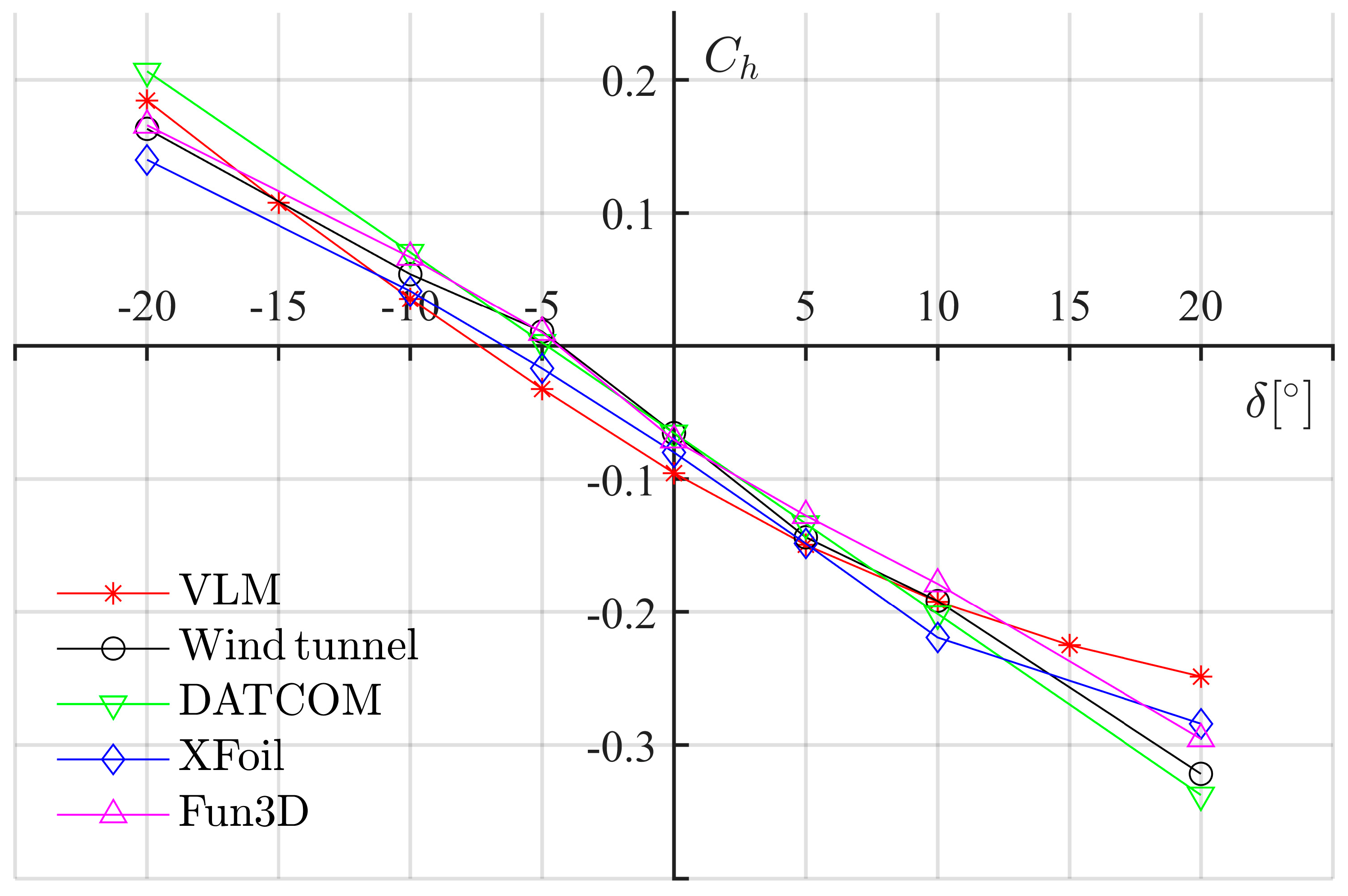
The hinge moment coefficients were estimated with the VLM solver, which is based on inviscid, irrotational, potential flow theory. Because the aerodynamic interactions of the control surface and wing can result in complex and detached flow, a VLM approach is not always valid. 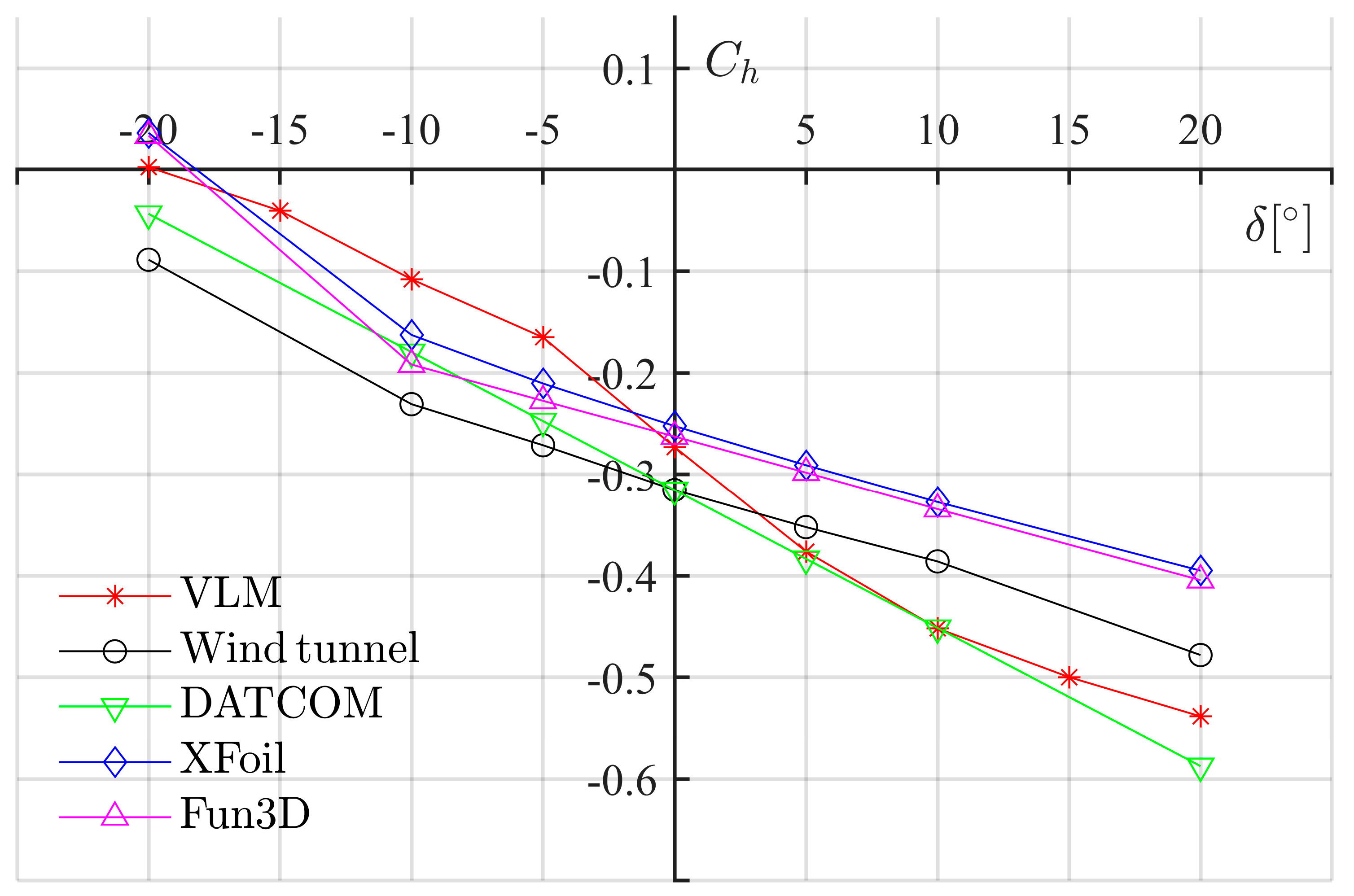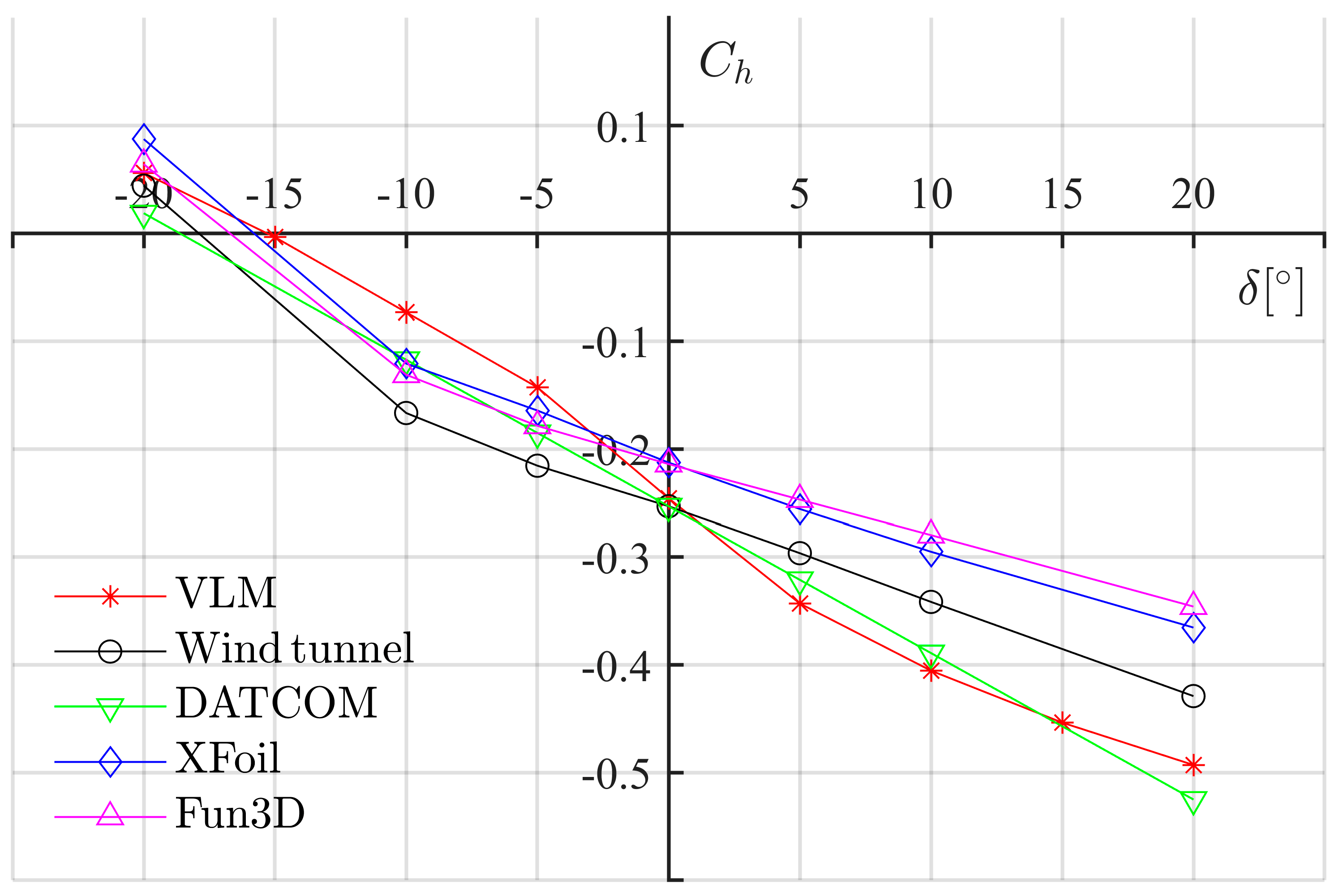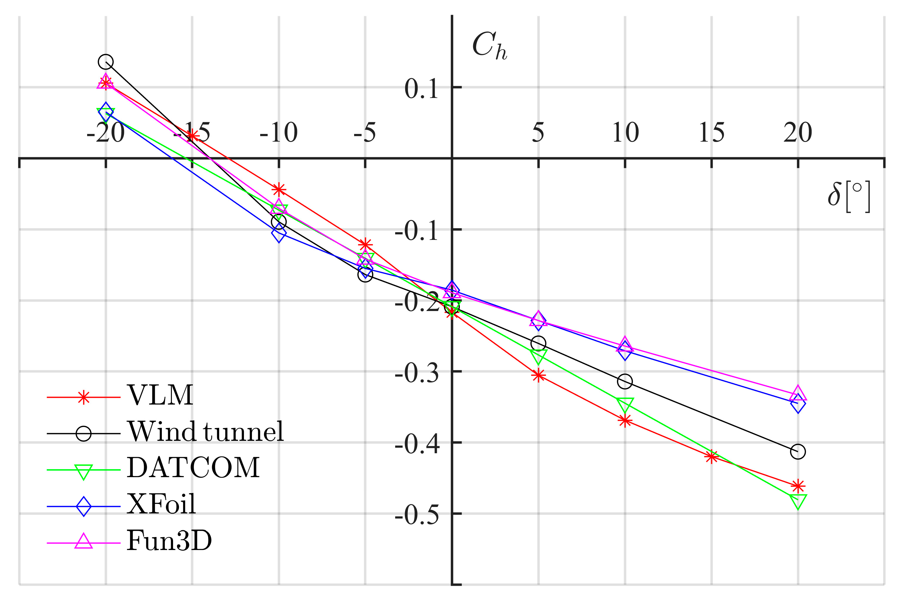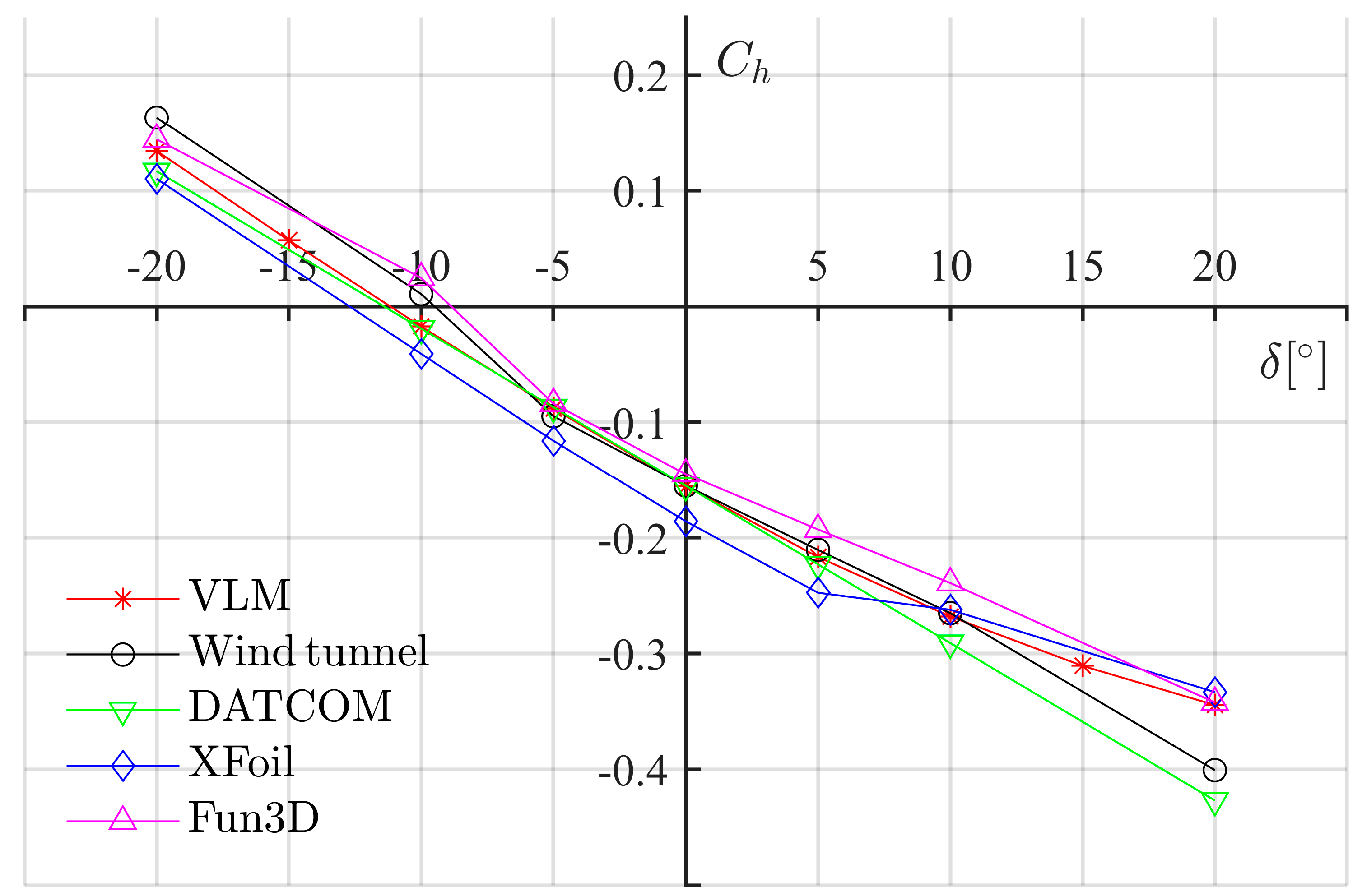Past work has shown that the linear relationship between hinge moment and deflection angle is reasonably accurate within a range of 15° surface deflection in subsonic flight conditions [11,19]. Thus, such surface deflection limits were maintained during the application of the framework and the hinge moment coefficients from the VLM solver are acceptable for subsonic aircraft whose flight conditions can satisfy the flow field assumption. In Appendix A, the hinge moments of a general aviation airfoil (GA(W)-1) with a plain flap under a series of deflection angles and attack angles were calculated by the VLM solver. The results were compared with that from a wind tunnel test, DATCOM (an empirical method), XFoil (no separated flow), and Steady Fun3D (Navier–Stokes solutions) for a cross-check [11,20]. The results show good comparison and indicate that the VLM solver is acceptable for the purposes of this study.

However, in the later stages of the design process, aerodynamic data from high fidelity CFD or wind tunnel experiments could substitute for more accurate hinge moment analysis, but these incur time and cost.

3.3. EMA Power Model

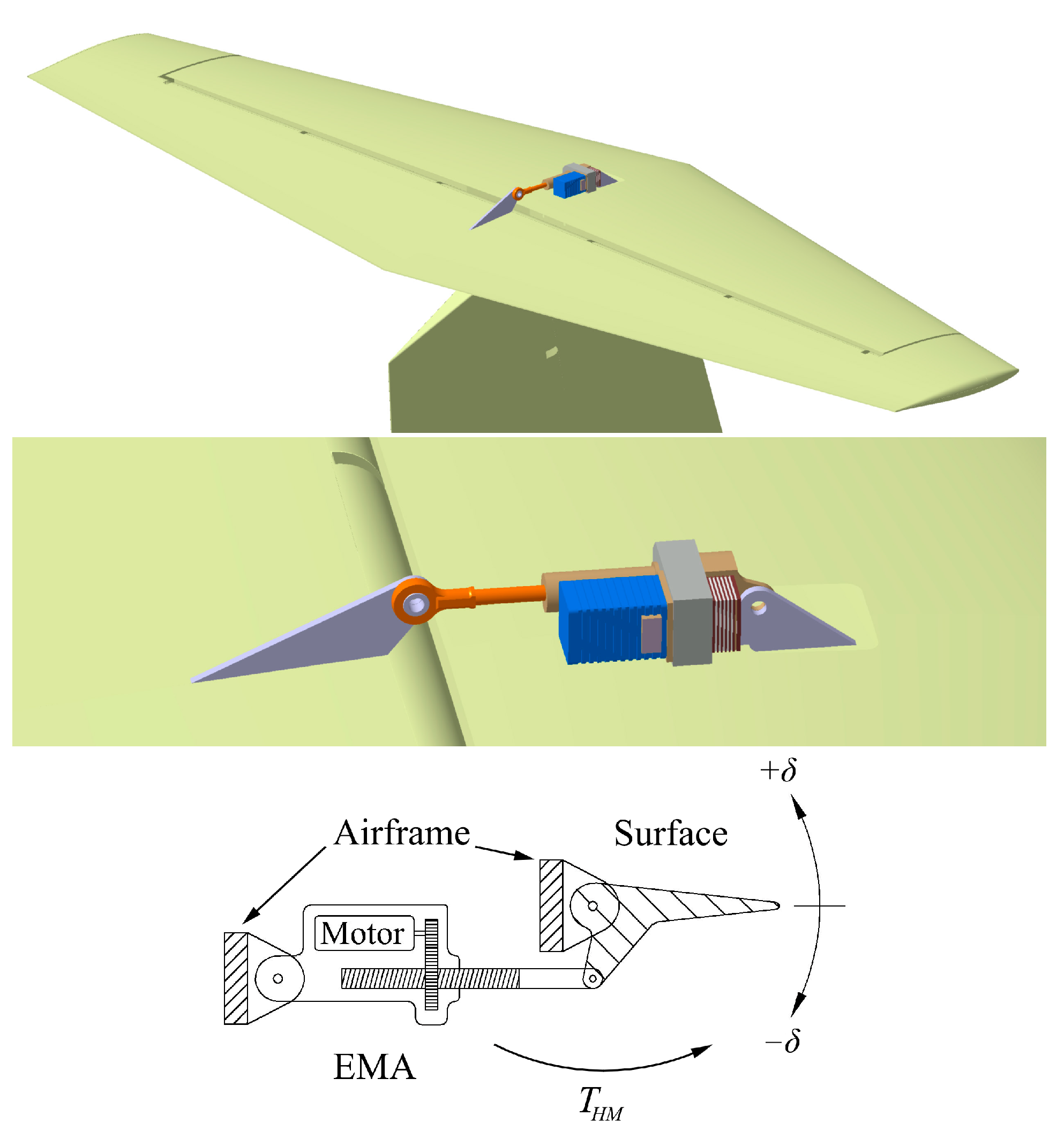
The ‘EMA Power Model’ estimates the power consumption of a single EMA for a given control surface deflection response and hinge moment. The mechanical transmission and motor sub-models were built to obtain transient electric power under different flight conditions and control laws. For this purpose, the EMA and linkage rods with a control surface were simplified to a single-DOF rigid-body mechanism, as mechanical compliance has been neglected. The moving parts include the gearbox, ball screw, control surface, and motor to convert motor shaft rotational motion to the surface deflect angles, as shown in Figure 3.

Figure 3. A schematic diagram of the simplified Single-DOF EMA model and surface actuation.

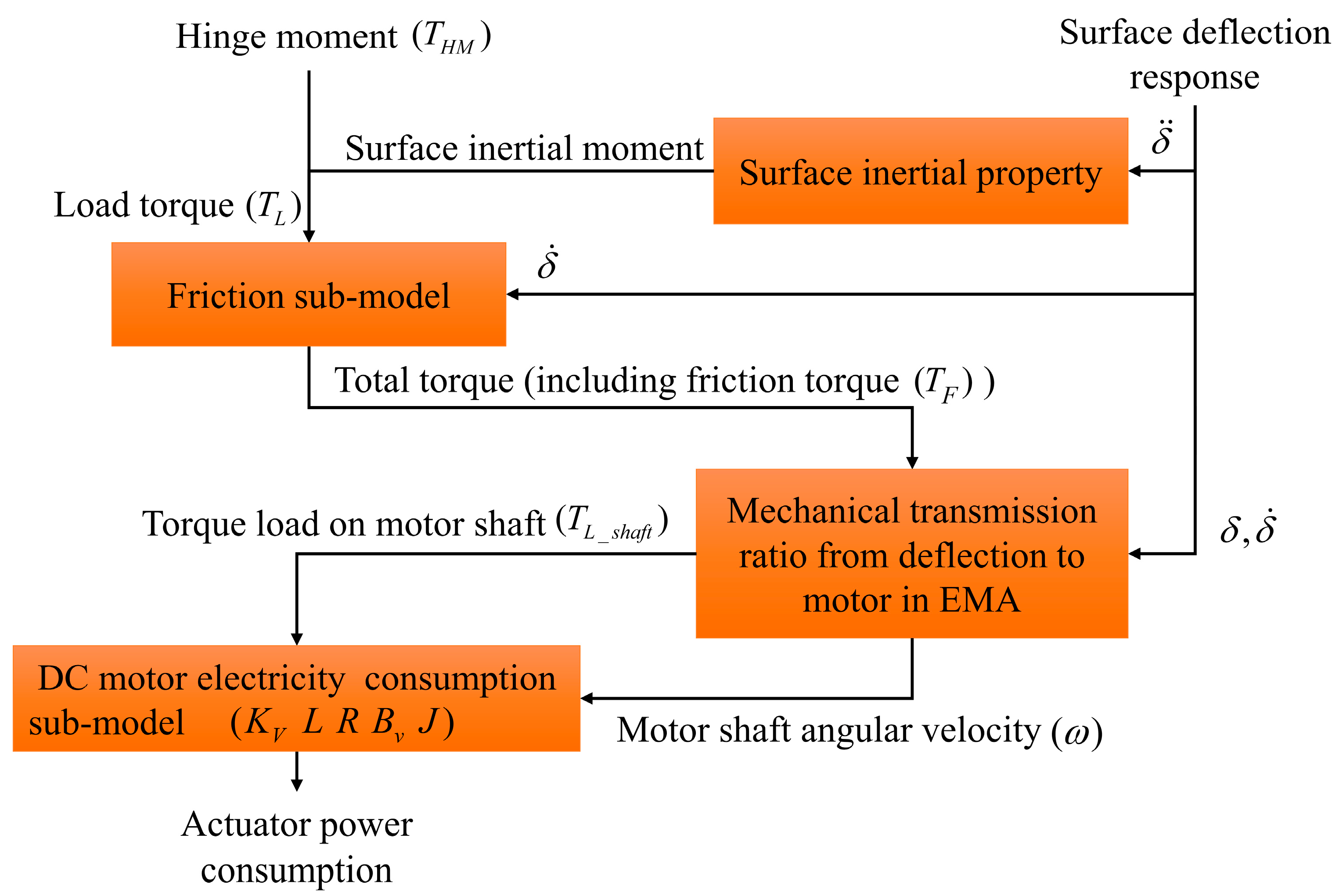
A top-level schematic describing the ‘EMA Power Model’ is shown in Figure 4. This schematic outlines the algorithm for the calculation of transient power from the surface deflection response. Considering the aim to simulate mission-level EMA power consumption, which can reflect different surface deflection motions and flight conditions, the friction estimation in mechanical transmission and motor electromagnetic characteristics model is a critical issue to address. The inertial effect of the surface and motor rotor and the non-linear effect in friction due to load directions are also considered.

Figure 4. Schematic showing the power consumption calculation in the EMA Power Model.

3.3.1. Friction Sub-Model in Mechanical Transmission

Friction is the dominant source of mechanical losses in both the motor and mechanical transmission. In this paper, Borello’s Friction Model was applied in which a set of parameters were used to model both load-dependent and load invariant friction torques [21,22]. It should be noted that the impact of temperature on friction was not considered in this paper, though its effect on friction has been widely studied.

According to Coulomb’s dry friction model [23], in the static case, the load invariant friction moment, $T_{Fi}$, is less than the maximum static (breakaway) value, $F_S$, and balances the driving and load torques to oppose the motion, while in the contrary case, it is equal to the dynamic value, $F_D$. The maximum static value, $F_S$, can be obtained by multiplying the static-to-dynamic friction ratio by the dynamic value, $F_D$. However, within the scope of this research (inverse simulation solving the driving torque, $T_d$, from the load torque, $T_L$, and deflection response), the load invariant friction moment is supposed to be $\left|T_{Fi}\right|=F_S=F_D$ and the driving torque $T_d$ is supposed to be no-less-than $F_S$ so as to avoid a statically indeterminate situation (two unknown variables, friction and driving torque). Under these assumptions, an arbitrary load torque, $T_L$, can be mapped to one single driving torque $T_d$. It should be noted that, in real circumstances (with mechanical compliance and the behaviour of real friction), only load torque magnitudes larger than a certain threshold (dictated by the position sensor tracking sensitivity) can be responded to by the EMA; therefore, the resulting power consumptions for the implemented model are conservative estimates, compared with the real conditions.

The direction of $T_{Fi}$ is opposite to the direction of rotation or the driving torque in the static case, as shown in Equation (2).

$$T_{Fi}=\{\begin{array}{c}{F}_D\cdot \mathrm{sgn}\left(\omega \right),\hspace{0.17em}\omega \ne 0\\ F_D\cdot \mathrm{sgn}\left(T_d\right),\hspace{0.17em}\omega =0\end{array},\hspace{0.17em}\left|T_d\right|\ge F_S=F_D$$

(2)

The load-dependent part, $T_{Fd}$, of the total friction torque is proportional to the load torque, $T_L$, and can be expressed by the transmission efficiency; however, it is worth emphasizing that the efficiency is related to the load direction relative to the deflection motion. When the load acts in the same direction as the deflection angular velocity, the efficiency is defined as the aiding efficiency, ${\eta }_A$. In the contrary case, when the load resists the deflection motion (including the static case), the efficiency is defined as the opposing efficiency, ${\eta }_O$. An equation for gear transmission, which relates aiding and opposing efficiencies is defined with an equivalent transmission, $\tau$, as shown in Equation (3) [24]. Due to the ball screw, this could only partly represent the real efficiency relationship in this hypothetical study. In future work, experimental work would be used to improve the accuracy of the mechanical efficiency model.

$${\eta }_A=\frac{2{\tau }^2{\eta }_O-{\tau }^2+\tau }{{\tau }^2{\eta }_O+\tau -{\eta }_O+1}$$

(3)

$T_L$ includes the hinge moment part and the inertial moment of the control surface. The surface inertial moments are calculated by the inertia around the hinge axis and surface deflection angular acceleration. The total friction torque, $T_F$, is then calculated with the efficiency under driving or resisting load, as shown in Equation (4).

$$T_F=T_{Fi}+T_{Fd}=\{\begin{array}{c}{F}_D+\left(1-{\eta }_A\right)\cdot \left|T_L\right|,\hspace{0.17em}\hspace{0.17em}\mathrm{under} \mathrm{aiding} \mathrm{load}\\ F_D+\left(\frac{1}{{\eta }_O}-1\right)\cdot \left|T_L\right|,\hspace{0.17em}\hspace{0.17em}\mathrm{under} \mathrm{opposing} \mathrm{load}\end{array}$$

(4)

The total friction torque and total load torque are added, and the sum is divided by the transmission ratio to obtain the torque load on the EMA motor shaft, $T_{L\_shaft}$. This is subsequently used for the electric power consumption calculation in the DC Motor sub-model.

3.3.2. DC Motor Electric Consumption Sub-Model

The DC Motor electric consumption sub-model can be seen as an inverse simulation model, in which, with a given shaft load torque and shaft angular velocity, the power consumption is obtained. The control surface load, along with the mechanical transmission friction, can be regarded as the external load on the motor and can be converted to the torque on the fast shaft by the transmission ratio. The motor shaft angular speed, $\omega$, is computed from the surface deflection response and mechanical transmission ratio. The air-gap torque of the motor ($K_{t}i$) can subsequently be obtained by the rotor dynamic equation, as shown in Equation (5).

$$\frac{d\omega }{dt}=\frac{1}{J}\left(K_{t}i-B_v\omega -T_{L\_shaft}\right)$$

(5)

The air-gap torque can be expressed as the product of the torque constant, $K_t$, and the transient current, $i$. The angular velocity and acceleration are the derivative and second derivative of the deflection response, respectively. The viscous friction of the rotor can be represented by the product of the damping factor and angular velocity. The damping factor can usually be obtained by the no-load rated characteristics of the selected motor, as in Equation (6).

$$B_v=\frac{K_t{i}_{noload}}{{\omega }_{noload}}$$

(6)

Typically, the motors in EMAs or servos are coreless (i.e., direct-current, with a permanent magnet stator inside). The electric consumption model of the motor is based on the theory of electromagnetic induction. The current differential equation of the motor is shown in Equation (7), where the motor transient input voltage can be obtained. The electric power consumption can subsequently be obtained by the product of the transient voltage and current, together with the efficiency assumed for the controller.

$$\frac{di}{dt}=\frac{1}{L}\left(V-iR-K_V\omega \right)$$

(7)

A schematic of the motor electric consumption sub-model is shown in Figure 5. This second-order sub-model involves two differential blocks; therefore, it is capable of accounting for transient power, including due to motor stall characteristics. Negative power consumption would indicate that the motor is operating as a generator. For this model, if this happens, the value is set to zero due to no power inverter being considered.

Figure 5. The schematic diagram of the DC motor electric consumption model.

Some limitations exist in the ‘EMA Power Model’ module described above. First, the surface deflection motion is limited to low-frequency responses, as the mechanical transmission, including the ball screw and linkage rod, are assumed as ideal rigid bodies; however, this is deemed acceptable, as the purpose of the module is to produce fast power estimates rather than detailed structural dynamics of the actuator. Secondly, the electrical power generation and distribution system, as well as the DC link management, are not included in the scope of the module. Rather, the impact of the actuator controller on energy consumption is represented by a power-efficiency factor. Thirdly, the temperature effects on the motor in EMA are not considered. During heavy-duty or frequent actuation of the EMA, a rising temperature could result in motor resistance and $K_V$ changes, which would, in turn, affect the power consumption.

3.4. Propulsion

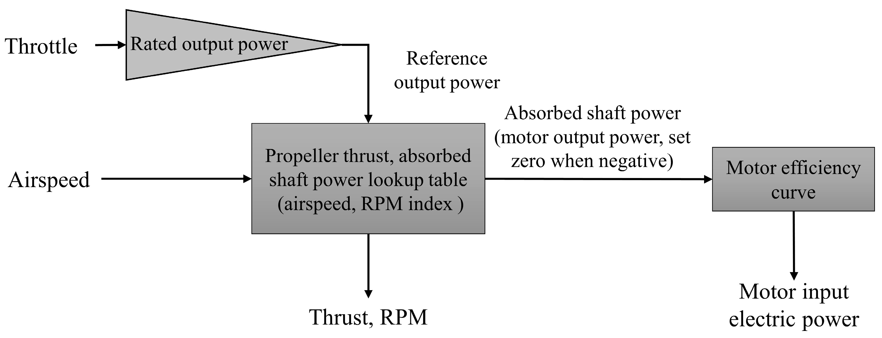
The ‘Propulsion’ module in this framework represents a model of a propeller driven by an electric motor. The module calculates the thrust at a given throttle position and airspeed, and also estimates the electric power consumption. The model was designed and verified with wind-tunnel testing to match the operational conditions of an electric aircraft from the literature [25]. In the module, the propeller performance is represented as two-dimensional lookup tables that provide thrust and absorbed shaft power values as output, with airspeed and RPM values as input. The electric motor controller can guarantee a linear relationship between shaft output power versus throttle position. Figure 6 shows a schematic of the module.

Figure 6. Data flow diagram for the propeller propulsion unit.

The motor reference output power is determined by multiplying the rated output power and throttle position (fraction from 0 to 1). Then, together with the airspeed, the corresponding RPM and thrust can be obtained from the lookup table interpolation. If the reference output power is larger than the absorbed shaft power at the maximum RPM, this absorbed shaft power should be regarded as the motor output power. Negative absorbed shaft power is set to zero, otherwise, the motor will function as a generator. The motor input electric power is obtained by the motor output power and the power efficiency curve, obtained from the datasheet [26].

3.5. Flight Control and Guidance

To comprehensively investigate the impact of the flight control and guidance algorithms on the EMA energy consumption, it is imperative that an appropriate guidance algorithm is used to ensure manoeuvres are performed consistently. The flight control philosophy in this work is closed-loop control of the 6DOF aircraft dynamics model to manoeuvre as required. The motion of the aircraft is decoupled in the longitudinal and lateral-directional dimensions. In order to investigate the characteristics of EMA electric consumption and its impact in real flight conditions, and especially to ensure industrial relevance, the flight control schemes were built with reference to ones commonly applied to conventional fixed-wing aircraft.

The attitude control loops were based on a classic proportional-integral (PI) controller with modifications to ensure improved dynamic performance in maintaining level flight (either in turning manoeuvres or under different airspeed). As shown in Figure 7, all three-axis control loops involve an airspeed scaling to keep the same aircraft dynamic response characteristics, as seen from the controller. By doing so within the specific range of airspeed, high-speed resonance or low-speed loose oscillation can be avoided. To compensate pitch control when the aircraft is in a bank, a roll compensation calculation block is included, which employs the measured bank angle to feed to the attitude error in the pitch attitude control loop.

Figure 7. Attitude control loop schematic diagram.

The two main functional targets for the yaw control loop are (i) eliminating sideslip when conducting coordinated turns and (ii) damping yaw oscillations. The sideslip angle is the direct variable used for sideslip elimination and is usually obtained by the weathercock sensor mounted on the aircraft nose; however, for some drones without a sideslip sensor, the acceleration information can be used instead to achieve a similar effect. As shown in Figure 8, in straight-and-level flight, the sideslip acceleration and yaw rate measurement inputs downstream from the high-pass filter are used to calculate rudder deflection to damp the yaw oscillation. When conducting coordinated turns, the measured bank angle is processed in the turn coordination calculation block and negatively feeds to the measured yaw rate.

Figure 8. Yaw control loop schematic diagram.

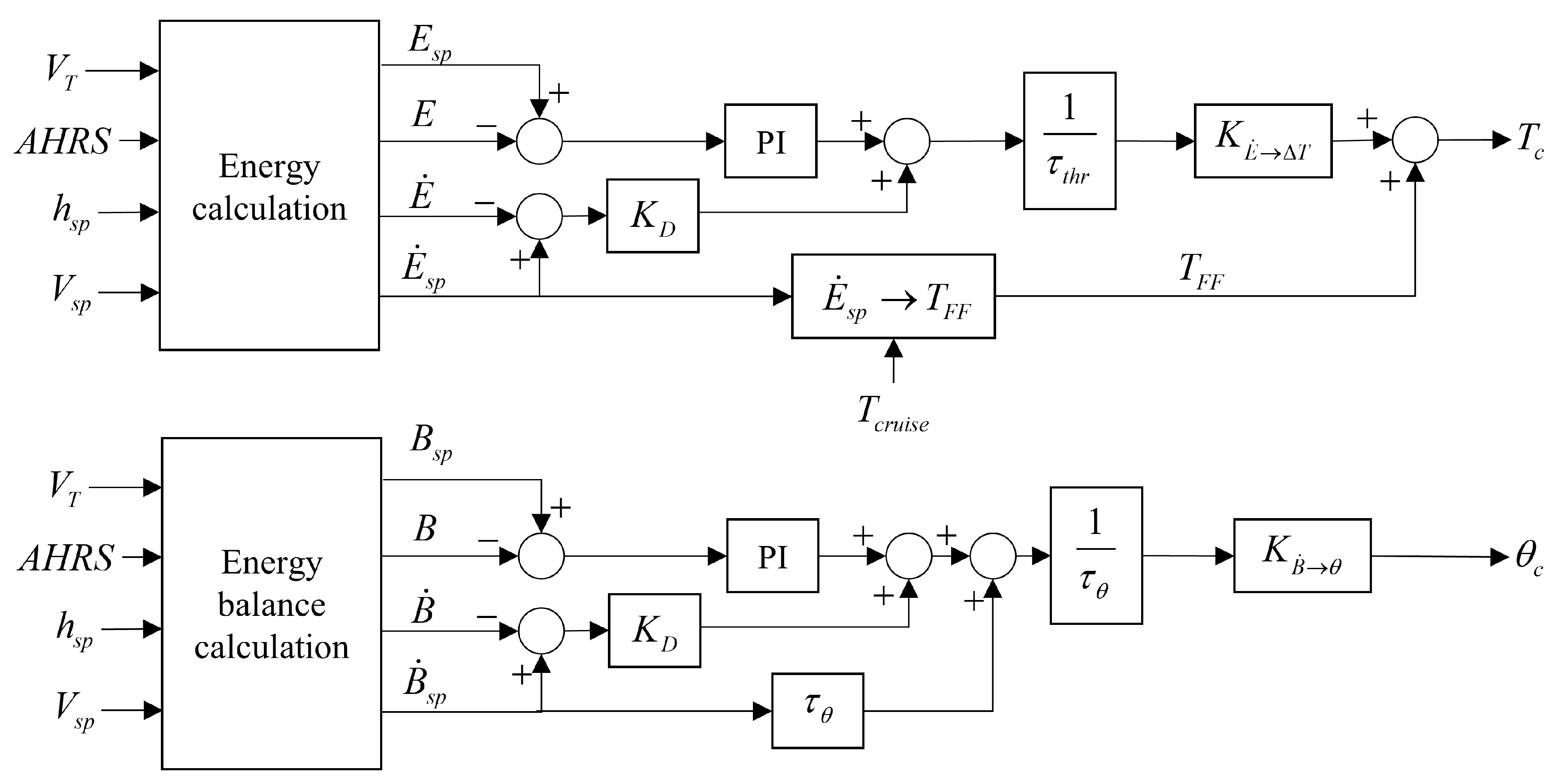
Altitude and speed control are implemented with the total energy control system (TECS), which is an integrated multi-input–multi-output (MIMO) algorithm decoupling altitude and speed control by regarding the total energy (kinematic and gravitational potential energy) and energy balancing states as the two separated targets. As shown in Figure 9, the current motion status (true airspeed $V_T$, attitude and acceleration information from attitude heading reference system (AHRS)), target altitude $h_{sp}$, and the speed setpoint, $V_{sp}$, are the multiple inputs to calculate throttle and demanded pitch angle, respectively.

Figure 9. The schematic diagram of the Total Energy Control System (TECS).

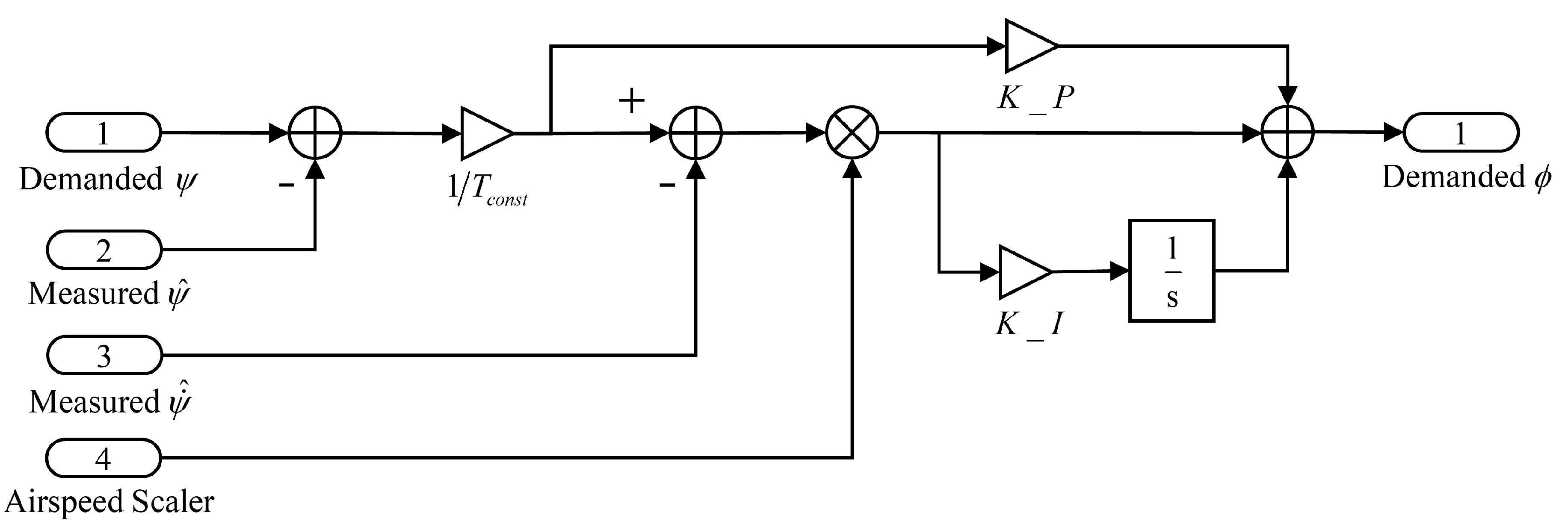
In this paper, the level trajectories are also taken as the study objective. According to the conclusion of previous work [4], trajectories with small turning radii will have larger EMA energy consumption. Moreover, for a tangential circular orbit connecting two intersecting straight flight paths, larger radii are equivalent to shorter trajectory lengths, which is expected to invoke less total energy consumption; however, for some applications, the aircraft need to pass by one waypoint and then switch to another, where the trajectories with smaller radii can be relatively shorter in length correspondingly. The presented guidance algorithm, as shown in Figure 10, was established in this manner to study the trajectory impact on total energy consumption. The PI controller is used to maintain and switch the heading direction to the next waypoint by generating a demanded bank angle.

Figure 10. Level navigation heading control loop schematic diagram.

4. Case Study: Small, All-Electric Fixed-Wing Aircraft

To demonstrate the capability of the framework, it was applied to a case study in which the impact on EMA energy consumption of turbulence intensity, parameters in the flight control algorithm, and the trajectory radius size were investigated.

4.1. Aircraft Parameters and EMA Sizing

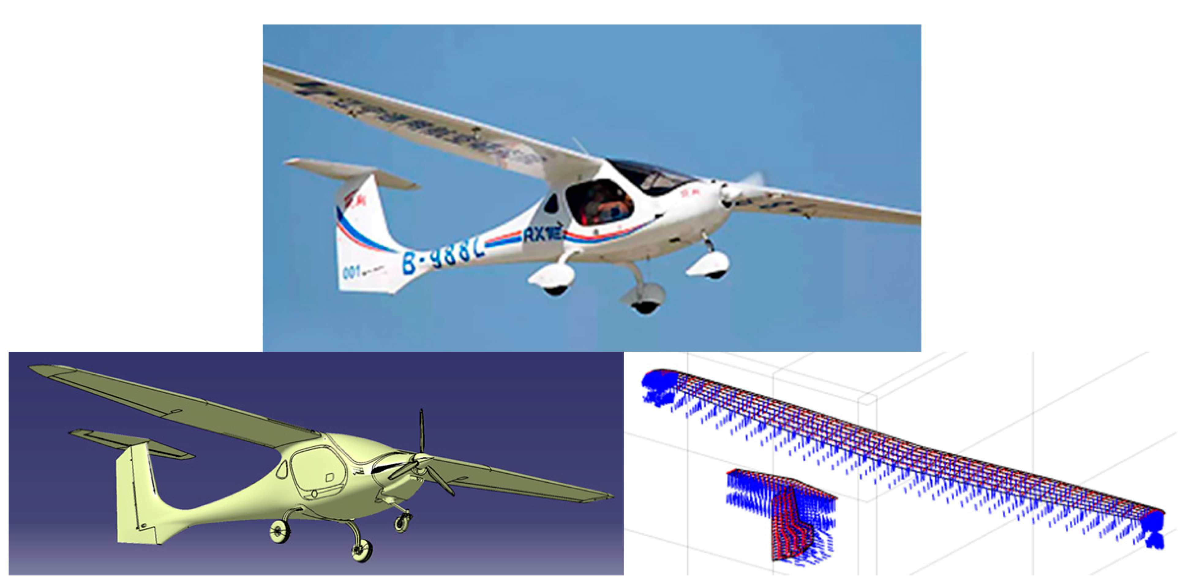
The application aircraft selected for the study was the two-seat all-electric RX-1E [27] (Figure 11). The salient characteristics of this aircraft are listed in Table 1. The selection of this aircraft was driven by its all-electric configuration and data availability, which made it feasible to demonstrate the framework. Although originally manually controlled, for this study, it was hypothetically equipped with flight control and guidance systems, and EMAs for control surfaces were incorporated to meet the deflection requirements.

Figure 11. Two-seat all-electric aircraft RX-1E and the vortex lattice distribution [27].

Table 1. Key characteristics of the RX-1E electric aircraft.

Wingspan (m)	Length (m)	Gross Weight (kg)	Cruise Speed (km/h)
14.5	6.6	500	110

To size an EMA, the rated power of the EMA motor and transmission ratio needs to be determined to match the surface requirements of the maximum hinge moment and deflection rates within the flight envelope. The designated deflection rate saturation should be large enough to avoid oscillation.

To illustrate the EMA sizing process, the aileron surface was selected as an example to calculate the maximum hinge moment. The hinge moment coefficient is maximal at $\alpha =10°,\delta =15°$ and the corresponding torque at the maximum airspeed of 40 m/s is calculated with Equation (1). The deflection rate saturation was set to 80°/s, which is close to other aircraft equipped with EMAs for surface actuation [28]. This maximum hinge moment estimate is imposed to ensure the hinge moment will not exceed the EMA-rated torque, even under the most severe condition in the simulation. From the perspective of conceptual design, the hinge moment sizing methods that take certification requirements into account should be considered.

The gearbox ratio, screw lead, and rod arm were sized iteratively to obtain a set of feasible parameters, which produce an actuation output that matches the deflection requirements. Commonly used values were selected for all the transmission parameters. Table 2 shows the resulting parameters of the sized EMA, as well as its characteristics that meet the requirements. The DC motor (Portescap 35GLT2R82-426E) was selected because of its suitable rated power and RPM capabilities [29].

Table 2. EMA sizing parameters and performance comparison.

Required Rate (°/s)	Deflection Rate (°/s)	Maximum Hinge Moment at 40 m/s (Nm)	Torque Output (Nm)
80	87	31.1	43.8
Transmission Parameters	Gearbox Ratio	Ball Screw Lead (mm)	Rod Arm (mm)
	14	16	68
MotorParameter	Continuous Torque (Nm)	No-Load Speed (RPM)	Rated Power (W)
	0.16	5439	150
Friction modelparameters	${\eta }_A$	${\eta }_O$	$T_{Fi}$(Nm)
	0.67	0.75	0.59

The friction model parameters are also listed in Table 2. The load invariant friction moment of 0.59 Nm is set to be one percent of the theoretically rated output torque (59 Nm) at zero-friction conditions, referenced to the hinge axis. The mechanical transmission efficiency at the opposing load was assumed to be 75%, and in the case of an aiding load of 67%, can be calculated according to Equation (3). For future work, experimental data could be used to revise the aforementioned parameters so that the model would accurately match the friction of a real EMA.

The moment of inertia of the surfaces, motor, and mechanical transmission are listed in Table 3.

Table 3. Moment of inertia of moving parts of the EMA system.

Moving Parts	Moment of Inertia [kg∙m2]
Aileron Surface (hinge axis reference)	9.10 × 10−3
Elevator Surface (hinge axis reference)	1.73 × 10−2
Rudder Surface (hinge axis reference)	1.79 × 10−2
DC Motor Rotor (motor shaft reference)	7 × 10−6
Gearbox and Ball Screw (motor shaft reference)	9 × 10−6

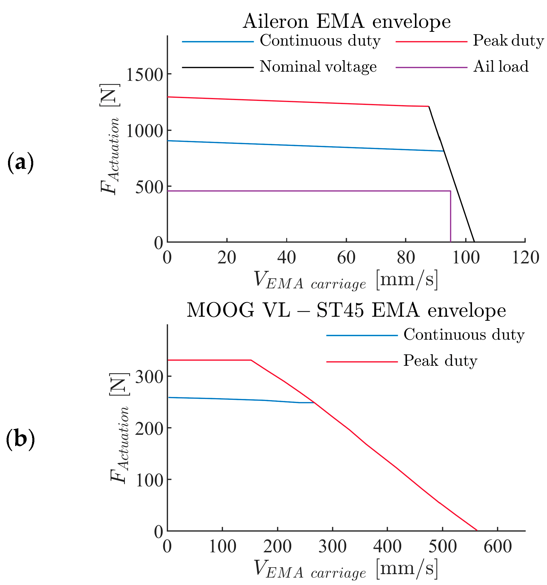
The performance envelope of the sized EMA module was generated using the rated parameters of the motor, including continuous current, peak-duty current, and nominal voltage. The aileron hinge moment was converted to the force on the rod for reference. The peak-duty and continuous current limits constitute the two horizontal lines in the aileron EMA envelope, representing the force limits. The nominal voltage forms the sloping line between the force limit and the rod translational velocity, which indicates that the load capability decreases with increasing EMA actuation velocity. The area below these limits constitutes the performance envelope. A comparison of the aileron EMA envelope with an off-the-shelf EMA is shown in Figure 12 [30]. The topology comparison of the envelopes indicates that the modelling approach properly captures the EMA limits required for a power consumption study.

Figure 12. (a) Performance envelope of the aileron EMA and the hinge moment load requirement; (b) performance envelope of the MOOG VL-ST45 EMA product.

The following sections introduce four EMA energy consumption impact studies involving proportional gains in the attitude control loop, turbulence intensity, proportional gain in the heading control loop, and trajectory radius, respectively.

4.2. Attitude Control Proportional Gains Tunning

Ideal attitude control is supposed to exhibit a rapid response, small overshoot, and a short settling time for a given attitude demand. The step response is a widely applied experiment to evaluate the dynamic performance of a control system. In the proposed case study, the proportional gains in the pitching and rolling attitude control loop were tuned under a demanded attitude step input.

The initial status before the step input is a straight-and-level flight at 30 m/s cruise speed. After a series of step response experiments, three pairs of proportional gains are selected for both longitudinal and lateral control. The dynamic response for these three pairs parameters, as shown in Figure 13 and Figure 14, can be described to have “moderate”, “normal”, and “aggressive” performance with the proportional gain increase. The rise in proportional gain leads to less response time and a larger overshoot, but the settling times for the gain settings of the three pairs are all shorter than five seconds.

Figure 13. Pitch control step responses at three proportional gains (1.5, 2.0, 2.5). The corresponding elevator EMA power consumption is also shown.

Figure 14. Roll control step responses at three proportional gains (0.7, 2.0, 4.0). The corresponding aileron and rudder EMA power consumption is also shown.

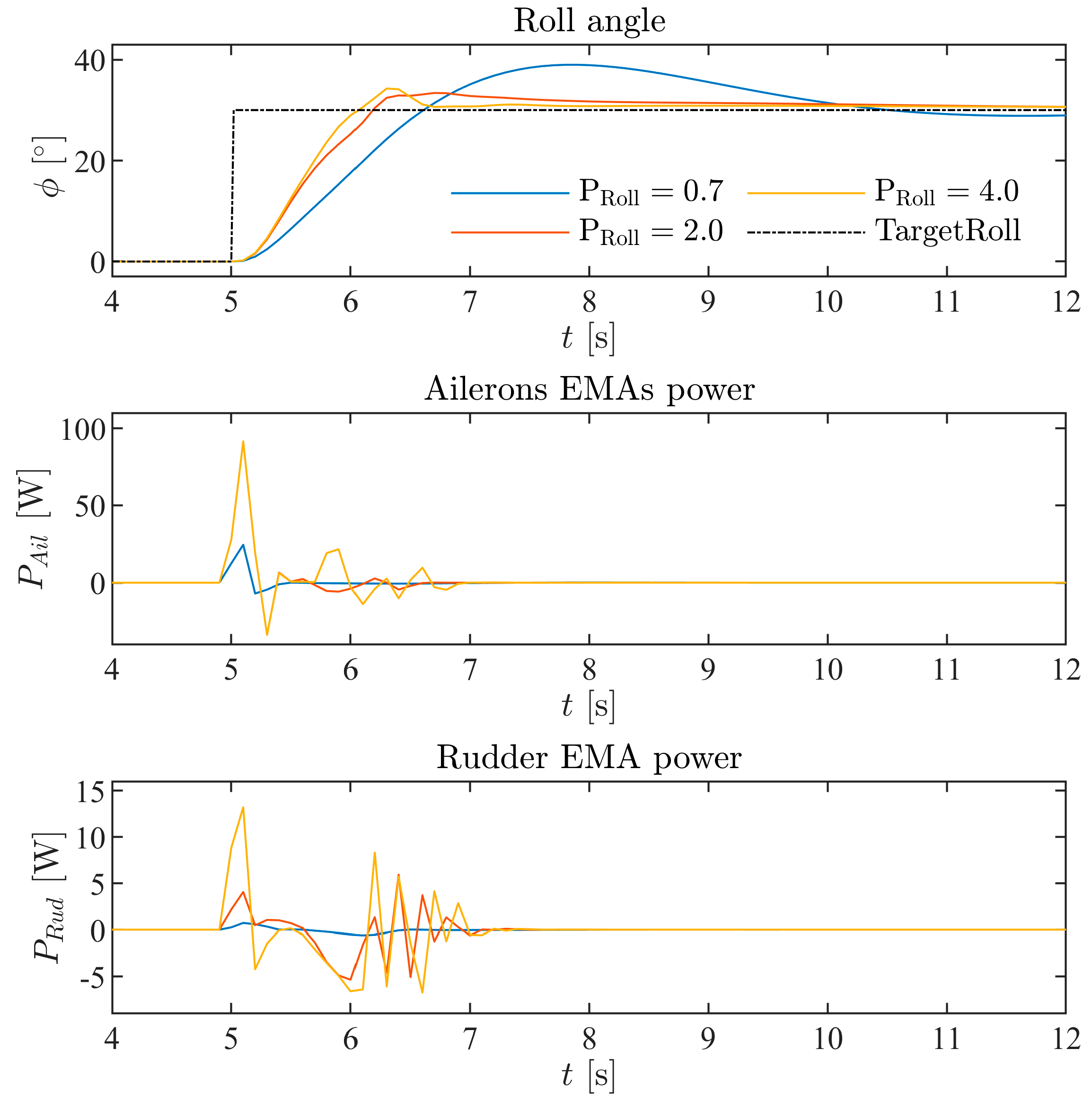
The EMA power features in step response are presented simultaneously with the attitude response. For both longitudinal and lateral-directional responses, a more “aggressive” proportional gain results in larger EMA power consumption. From the longitudinal step response in Figure 13, it can be seen that a larger pitch proportional gain corresponds to a larger amplitude in pitch oscillation, which in turn results in a larger elevator deflection as well as EMA power consumed. For the roll step response, as shown in Figure 14, a larger proportional gain in the lateral control loop renders the roll response ‘stiffer’, especially as it relates to overshooting. This leads to additional significant rudder EMA power consumption. The basic EMA power consumption characteristics in step response provided instructively supported the more comprehensive EMA power impact studies provided next.

4.3. Turbulence Impact

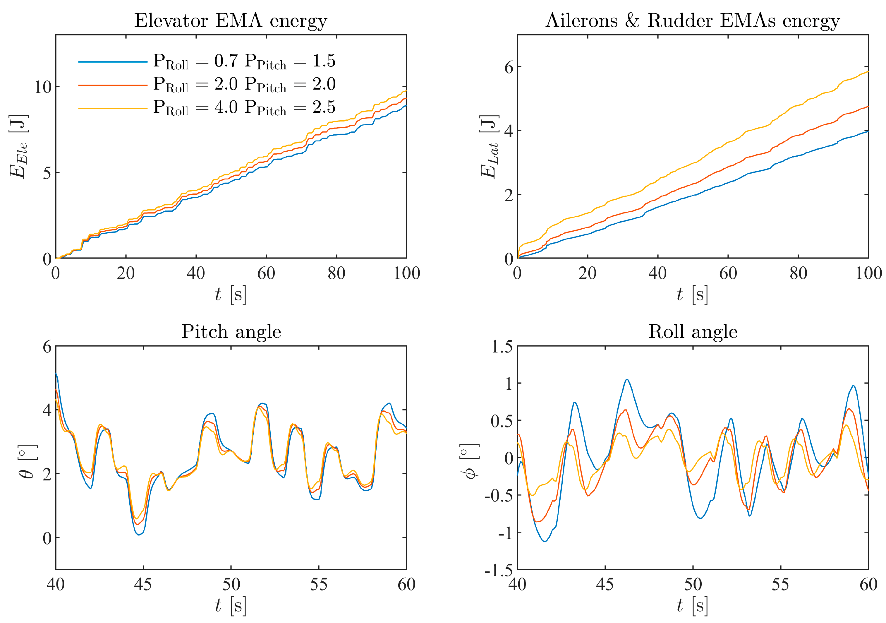
Atmospheric turbulence is intuitively expected to impact EMA electric power, because the flight control system frequently generates surface deflection commands to eliminate attitude error. The EMA energy consumption study with respect to turbulence impact was conducted in two steps. First, the aircraft was set to maintain straight-and-level flight in turbulent air with a constant intensity (10 m/s), while the above three sets of selected proportional gains were set in the attitude control loop to analyse the EMA energy consumption difference. Secondly, the proportional gains were set at the “normal” value ($P_{Roll}=2.0\hspace{0.17em}{P}_{Pitch}=2.0$) and the EMA energy consumption impacts from three turbulence intensities (5 m/s, 10 m/s, 15 m/s) were compared.

Figure 15 shows the aircraft EMA energy consumption and attitude response for a 10 m/s turbulence intensity at different attitude proportional gains. The results for longitudinal and lateral-directional dimensions are presented separately. The fluctuations in pitch angle of three sets of parameters are all less than 5° and, for the roll angle, the amplitudes are less than 3°. It can be observed that the larger attitude proportional gain corresponds to larger EMA energy consumption and less fluctuation amplitude in attitude control, which is consistent with the results of the aforementioned step response. Moreover, in both the longitudinal and lateral-directional dimensions, the attitude fluctuation amplitudes are approximately inversely proportional to the EMA energy consumption.

Figure 15. Longitudinal, lateral-directional EMAs energy consumption, and attitude response in turbulence (at 10 m/s intensity) for three proportional gain settings in the attitude control loop.

The EMA energy consumption and attitude plots of Figure 16 show the turbulence intensity impact for when the attitude control proportional gains are set at “normal” values ($P_{Roll}=2.0\hspace{0.17em}{P}_{Pitch}=2.0$). It shows an approximate linear growth in EMA power consumption and attitude fluctuation with the intensity increase in the Dryden atmospheric turbulence model. This increase in energy consumption is caused by the increase in disturbance amplitude, resulting in larger and more frequent deflections to maintain level flight.

Figure 16. Longitudinal, lateral-directional EMAs energy consumption, and attitude response for different turbulence intensities (5 m/s, 10 m/s, 15 m/s).

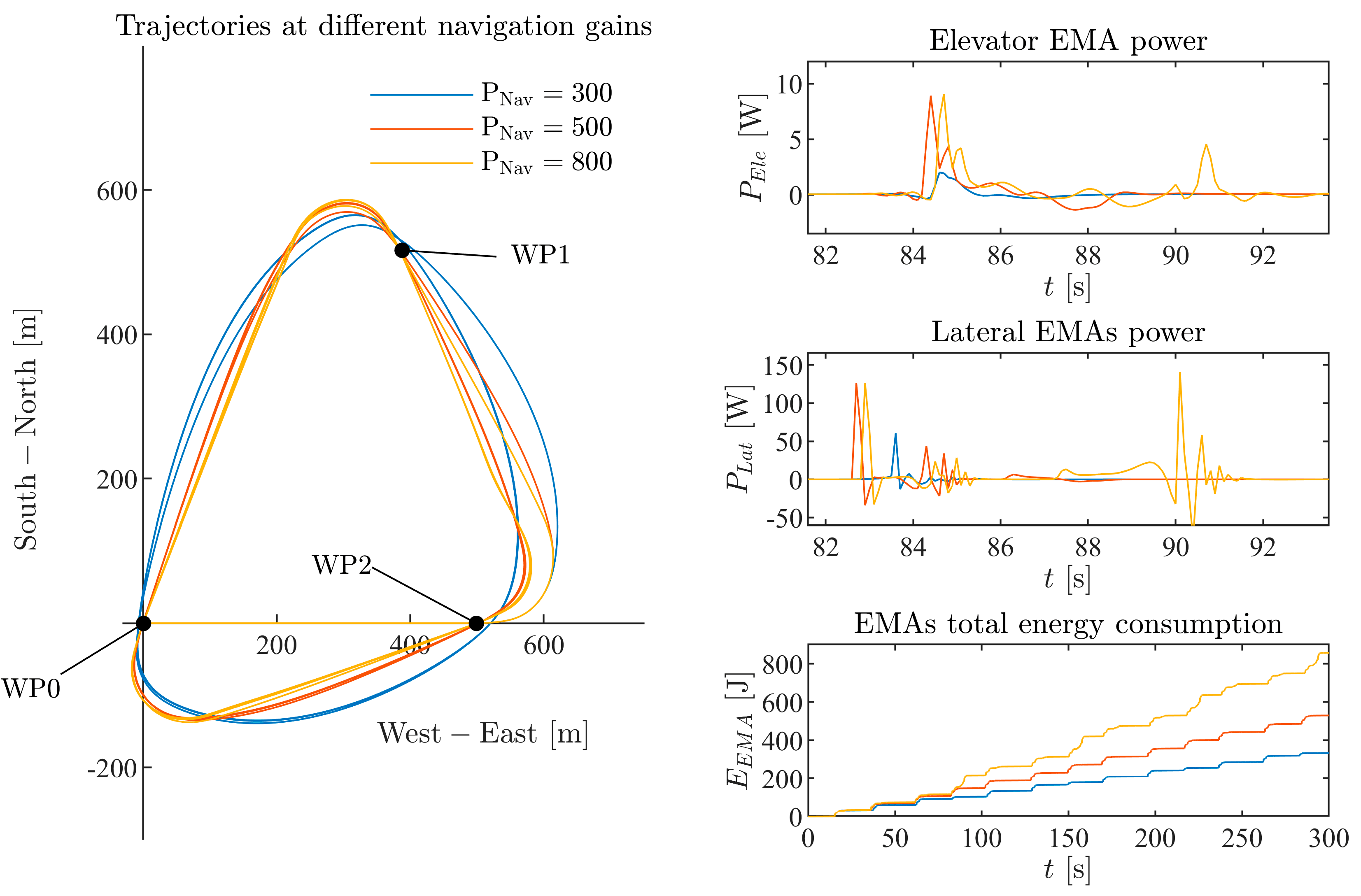
4.4. Proportional Gain in Heading Control Loop

The dimensionless proportional gain in the heading control loop, as shown in Figure 10, reflects the heading control stiffness in level navigation. To demonstrate the impact of this parameter on the EMA power consumption, a waypoint fly-over flight mission was set up to enable the aircraft to fly towards three subsequent designated waypoints. Once the distance to the current heading waypoint is less than a threshold (20 m), the target waypoint switches to the next one. During the simulation, the altitude and velocity are set to stay at the initial, constant values.

The trajectories for the three heading control gain settings and the resulting EMA power consumption are shown in Figure 17 (The power consumption graph only shows one turn). The maximum bank angles for all these three trajectories are all set at 45°. With the increase in heading control gain, the autopilot steers the aircraft more aggressively toward the target heading and is accompanied by an increase in EMA electric consumption. The longitudinal and lateral-directional EMA power consumption both increase significantly at the beginning of each turning manoeuvre, with the gain increasing from 300 to 500. At a heading control gain of 800, a slight overshoot emerges at the end of each turn. A notable influence on the power consumption is also noticed for this gain setting.

Figure 17. Trajectories and EMA power consumption of the RX-1E at different heading control gain settings.

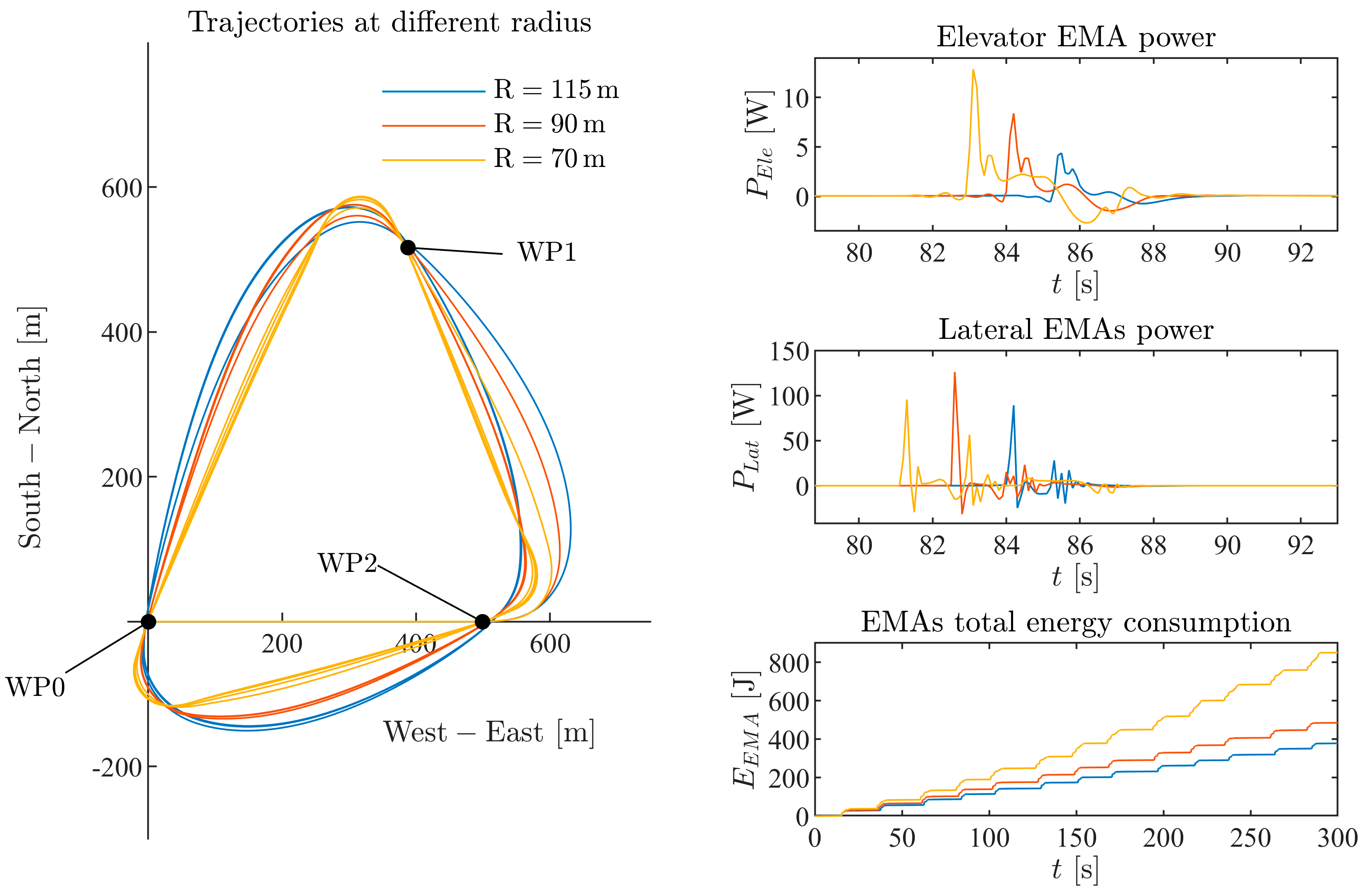
4.5. Effect of Trajectory Radius

The trajectory radius impact was studied for the same waypoint fly-over mission, with all of the other parameters held at the same values as before. The radius of the trajectory was varied by adjusting the maximum roll angle limit. Results for trajectories with radii of 70 m, 90 m, and 115 m, along with the associated EMA power consumption, are presented in Figure 18. As can be seen, as the radius increases, the trajectories gradually become more circular, and their length increases as well.

Figure 18. Trajectories and EMA power consumption at turning radii of 115 m, 90 m, and 70 m.

The decrease in trajectory radius results in a significant increase in elevator EMA power consumption. In order to maintain altitude, the increase in bank angle requires a corresponding increase in the angle of attack, which requires larger elevator deflection. At the maximum of the aileron and rudder EMA power consumption, three radii are similar in magnitude, but smaller radii require more power to level the aircraft; therefore, the total EMA electric power consumption shows a significant increase as the trajectory radius decreases.

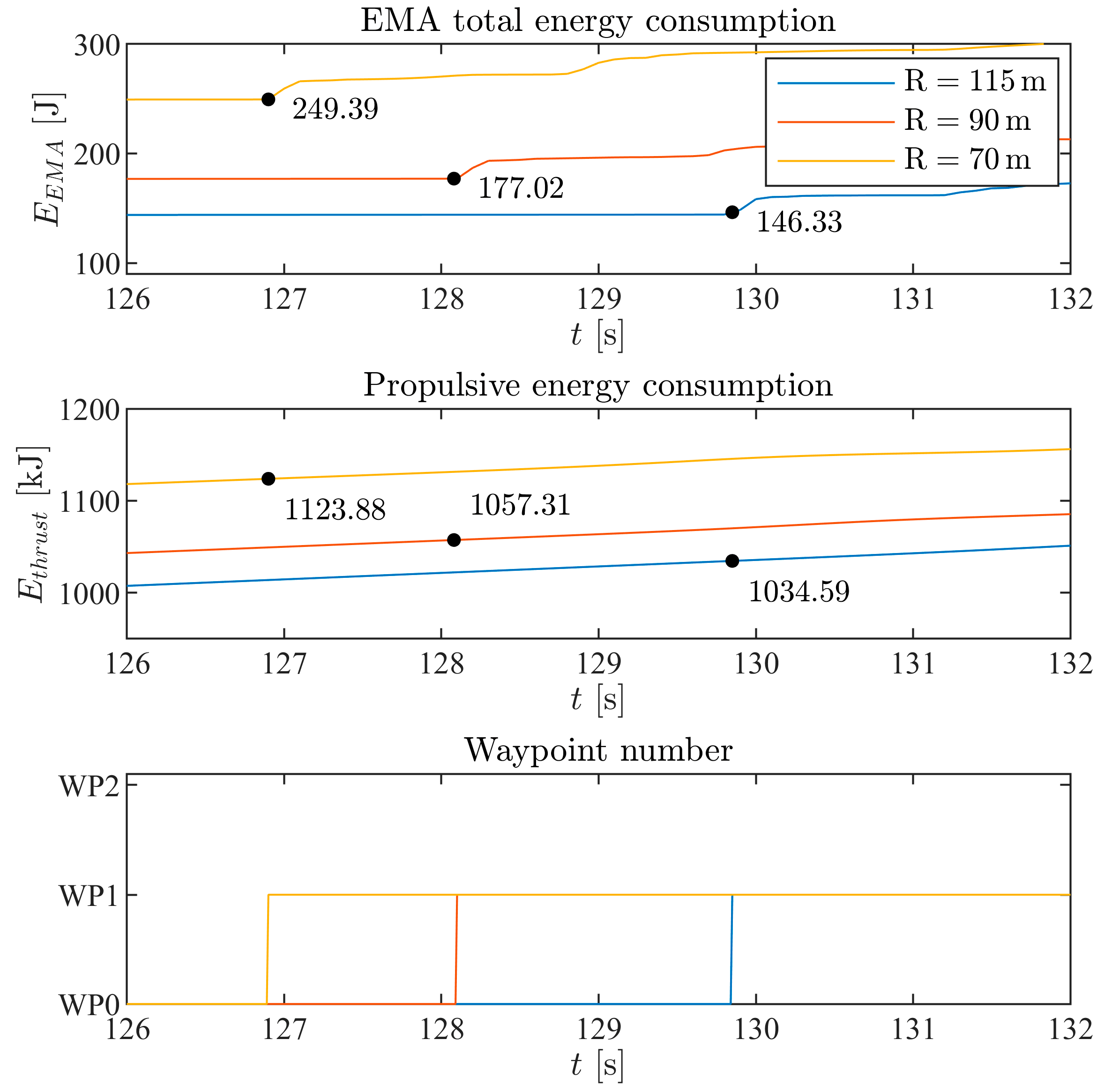
However, if the propulsion energy consumption is considered, even though the trajectory for 70 m radius is the shortest and fastest, its electric power consumption appears to be larger compared with the other two cases, both for the EMAs and propulsion. Figure 19 shows the combined propulsive and EMA energy consumption as the aircraft flies over waypoint WP1.

Figure 19. Energy consumption comparison at the same waypoint for the EMA and propulsion units.

This can be explained as follows: when the aircraft turns with a large bank angle (due to the small, enforced waypoint radius), it requires extra thrust to overcome the increased induced drag; therefore, even though the trajectory length and flight time are related to the amount of energy consumed, in this case, the shorter trajectories correspond to higher EMA and propulsive power consumption instead. This counterintuitive result reveals the need for a fully integrated airframe systems simulation when conducting an energy-efficiency trajectory investigation.

Although the EMA energy consumption is almost negligible compared with the propulsive cost, estimating its magnitude is still important as it directly affects the electric power supply and power electronics sizing. This includes the important sizing cases for emergency backup power, where the basic flight control energy requirement and an energy-efficient flight control strategy may be considered for some aircraft types. Moreover, the proposed simulation tool can be applied to a case where the flight control EMA power consumption would have a nonnegligible effect on the whole aircraft. For example, high altitude long endurance (HALE) solar-powered unmanned aircraft are exposed to significant levels of turbulence, for which the EMA energy losses may need to be comprehensively considered when the main energy reservoirs are sized.

5. Conclusions and Future Work

In this paper, a generic simulation framework was presented to investigate mission-level electromechanical actuator (EMA) energy consumption. The framework enables the user to analyse transient EMA power for different flight control algorithms, mission trajectories, and flight conditions, among other factors.

The core of the framework encompasses physics-based EMA power estimators linked with a 6DOF dynamics and flight control simulation module. The electromagnetic motor relationship, actuator mechanical friction model, and control surface deflection inertia are all taken into consideration for this no-regeneration inverse EMA simulation. The mechanical transmission is assumed to be rigid, and the application of Borello’s friction model excludes the sub-breakaway stiction to avoid a statically indeterminate situation. This enables a comprehensive calculation of actuator power at different conditions. The aerodynamics and control surface hinge moments were modelled with a vortex-lattice method-based rapid aerodynamics estimation program. Although additional care is required in some low Reynolds number cases, it enables the study of more types of aircraft compared with empirical methods. This is particularly relevant and useful during the early aircraft design stages.

To demonstrate the capabilities of the simulation tool, a case study to investigate the EMA energy consumption of a small all-electric fixed-wing aircraft was devised. In this case study, turbulence intensity and selected parameters of the flight control and guidance system were varied to investigate their impact on the EMA energy consumption. The results of the case study can be summarized as follows:

• The proportional gains in the attitude control loop directly impact the EMA electric power consumption. In the step response tests for three sets of gains, it was shown that a more aggressive proportional gain setting will lead to a corresponding increase in EMA power consumption.
• The atmospheric turbulence intensity can have a non-trivial impact on the EMA electric energy consumption. There is an approximately linear relationship between these two quantities. Under the same turbulence conditions, the increase in the attitude control proportional gain leads to larger power consumption but less fluctuation in attitude.
• Increases in the gains in the heading control loop will result in larger EMA power consumption. This applies to both the longitudinal and lateral-directional dimensions. Overshooting in level turning due to a large heading control proportional gain setting also caused the aileron and rudder EMA power consumption to increase.

The impact of trajectory radius was also investigated by varying the roll angle constrains in the three-waypoint fly-over mission. Higher turning rates resulted in significant increases in the EMA energy consumption. It was also found that higher EMA energy consumption was associated with higher propulsion energy consumption. Although higher turning rates resulted in shorter trajectories and flight times, the total energy consumption was generally higher than for trajectories with lower turning rates. This was attributed to an increase in the induced drag.

These results demonstrate the types of studies that can swiftly be performed with the simulation tool. Due to the comprehensive modelling approaches followed, the tool can extensively support the design of power electronics and secondary power supply, especially during the early design stages. Furthermore, it enables the user to study the effects of several types of flight conditions and mission trajectories on energy consumption, which may aid in managing trajectories with overall improved energy efficiency.

Two key avenues for future work have been identified. The first is to supplement VLM for overall aircraft aerodynamics with validated methods for hinge moment estimation at lower Reynolds numbers. The second is to include the influence of temperature on the motor electric consumption model, for example, with temperature-related motor parameters.