Abstract
Performing clustering analysis on a large amount of historical trajectory data can obtain information such as frequent flight patterns of aircraft and air traffic flow distribution, which can provide a reference for the revision of standard flight procedures and the optimization of the division of airspace sectors. At present, most trajectory clustering uses a single clustering algorithm. When other processing remains unchanged, it is difficult to improve the clustering effect by using a single clustering method. Therefore, this paper proposes a trajectory clustering ensemble method based on a similarity matrix. Firstly, a stacked autoencoder is used to learn a small number of features that are sufficiently representative of the trajectory and used as the input to the subsequent clustering algorithm. Secondly, each basis cluster is used to cluster the data set, and then a consistent similarity matrix is obtained by using the clustering results of each basis cluster. On this basis, using the deformation of the matrix as the distance matrix between trajectories, the agglomerative hierarchical clustering algorithm is used to ensemble the results of each basis cluster. Taking the Nanjing Lukou Airport terminal area as an example, the experimental results show that integrating multiple basis clusters eliminates the inherent randomness of a single clustering algorithm, and the trajectory clustering results are more robust.
1. Introduction
In response to the challenges of airspace congestion, flight delays, and other challenges brought about by increasing traffic volumes to improve the level of safety, efficiency, and sustainability of the air traffic system, Europe launched the Single European Air ATM Study (SESAR), the United States launched the Next Generation Air Transport System (NextGen), the International Civil Aviation Organization (ICAO) built the Aviation System Block Upgrade (ASBU) framework, etc. One of the common key technologies to all these automated systems is the ability to analyze and process large numbers of trajectory records scientifically and efficiently. The reason is that historical trajectory data contains a lot of potentially useful information. At present, the most commonly used and efficient method to mine potential information from a large amount of trajectory data is to perform clustering analysis on trajectories. Through clustering analysis, the frequent flight patterns of aircraft, air traffic flow situation, airspace usage, etc. can be known, which can reflect the flight tendency of aircraft and the control habits of controllers to a certain extent. It can provide a reference for the optimization of the division of airspace sectors and for the controller to make control decisions. In addition, many scholars regard trajectory clustering as one of the key steps in trajectory prediction. By classifying similar trajectories into one category in advance, and then establishing a prediction model for each category of trajectories separately, the prediction results can be more accurate and robust [1,2].
Trajectory clustering methods can be roughly divided into four categories, including clustering based on the partition, density, grid, and probability models. All of these clustering methods can be used to cluster the trajectories and can achieve certain results. Among the partition-based clustering methods, the K-means clustering algorithm has higher computational efficiency than other algorithms and does not need to spend a lot of time debugging parameters. The only parameter that needs to be input is the number of clusters, which has the advantage of being easy to implement. Therefore, it is adopted by most scholars [3,4,5,6,7,8]. Barrat et al. [7] used K-means to acquire the center trajectories, and then constructed a Gaussian mixture model based on the center trajectories to achieve accurate inference and generate more realistic trajectories. Ayhan et al. [6] considered that treating a trajectory as a whole may lead to overfitting, and cannot find representative trajectories, so they proposed a clustering framework of aircraft trajectories based on the tasks of division, clustering, and merging. Use a set of multi-dimensional trajectory points associated with a particular flight, divide them according to flight phase, cluster them individually with the K-means algorithm, and combine them. In addition, in contrast, the K-medoids algorithm, in addition to being relatively slow, selects centers from the actual data points within the cluster. Therefore, it is not sensitive to outliers [9,10]. Kenefic et al. [10] adopted the K-medoids algorithm based on the minimum description length and the Frechet distance, which can be generalized to the clustering problem of datasets with arbitrary shapes.
The most popular method in density-based clustering is Density-Based Spatial Clustering of Applications with Noise (DBSCAN). Most density-based trajectory clustering is implemented by the DBSCAN algorithm or improved implementation of the algorithm [11,12,13,14]. Olive et al. [12] first used the DBSCAN algorithm to identify the initial set of clusters and outliers, and then adopted the progressive clustering method. For the classes that cannot be well separated, the clusters were refined by applying the DBSCAN algorithm to each flow again. Verdonk et al. [13] proposed an algorithm RDBSCAN based on the recursive application of DBSCAN, which recursively creates a hierarchy that enables a more customized classification of outliers. Hierarchical clustering creates a hierarchical decomposition of a given set of objects. Depending on how the hierarchical decomposition is formed, hierarchical methods can be classified as agglomerative or divisive methods [15,16,17]. Zhang et al. [16] introduced an agglomerative hierarchical clustering method that builds a hierarchical structure based on a set of centers, aiming to improve computational efficiency when dealing with massive data. Trajectory clustering based on probabilistic models attempts to find the best data model to fit the given data, and assumes a model for each cluster, looking for the best fit of the data to the given model. Gaussian mixture models are often used to fit the data in probabilistic model-based trajectory clustering [18,19]. Zeng et al. [18] considered that the Gaussian mixture model could give the class probability to which each trajectory belongs, so they used the Gaussian mixture clustering method to identify and mine the prevailing flight patterns of aircraft in the terminal area.
Since each clustering method has its advantages and limitations, we can ensemble a variety of clustering methods to give full play to their respective advantages, that is, clustering ensemble, which has become a better direction of research in current trajectory clustering [20,21,22,23,24]. In addition, since deep learning exhibits great autonomy, it is also a valuable research direction in the future to use deep learning to automatically learn the final clustering results from massive data [18]. Olive et al. [25] introduced two deep trajectory clustering methods implemented with autoencoders, which cluster high-dimensional data according to their representation in a low-dimensional space. In addition, Pasi Franti et al. [26] proposed a prototype swap clustering method, clustering by swapping a series of prototypes (cluster center trajectories) and using K-means to fine-tune the positions of these prototype trajectories. In essence, this method only has one more prototype trajectory swap step than K-means, but it can achieve high-quality clustering through a random search strategy.
At present, most trajectory clustering uses a single clustering algorithm. When other processing remains unchanged, a single clustering method encounters a bottleneck in improving the clustering effect. In addition, when the dimension and length of the data are large, it is difficult for most clustering algorithms to maintain high computational efficiency on massive data sets. In addition, most of the current trajectory clustering is based on the attributes such as longitude, latitude, and altitude of the trajectory. How to make full use of the existing attributes is also a problem that should be paid attention to in the clustering.
In this paper, a clustering ensemble method of aircraft trajectory based on a similarity matrix is proposed. To efficiently utilize the existing attributes, a derived attribute that can describe some inherent law of the data is constructed. To improve computational efficiency, the Stacked autoencoder is used to learn efficient feature representations of the trajectories, which are used as inputs to subsequent clustering algorithms. Multiple different basis clusters are used to generate diverse clustering results, and the clustering ensemble method based on a similarity matrix is used to ensemble each clustering result to obtain more robust results. Summarizing the main contributions of this paper are as follows: (a) The derived attributes that can effectively characterize the trajectory shape information are constructed from the existing features empirically. (b) As far as we know, this paper is the first time to use a clustering ensemble to solve the problem of trajectory clustering, which provides a new way for related researchers to solve the problem of trajectory clustering. The clustering ensemble method based on a similarity matrix is used to ensemble the results of each base cluster, which eliminates the inherent randomness of the single clustering algorithm itself.
The rest of the paper is organized as follows. Section 2 describes the theory and implementation process of the trajectory clustering ensemble method based on the similarity matrix proposed in this paper. Section 2.1 introduces the derived property of the angle of construction, Section 2.2 introduces the process of learning trajectory features from the original data using the stacked autoencoder, and Section 2.3 describes the clustering ensemble method based on the similarity matrix, which is the focus of this section and the whole article. Section 3 presents the experimental results and discusses the superiority and effectiveness of our method. Finally, Section 4 summarizes the work carried out in this paper and looks forward to future research directions.
2. Methodology
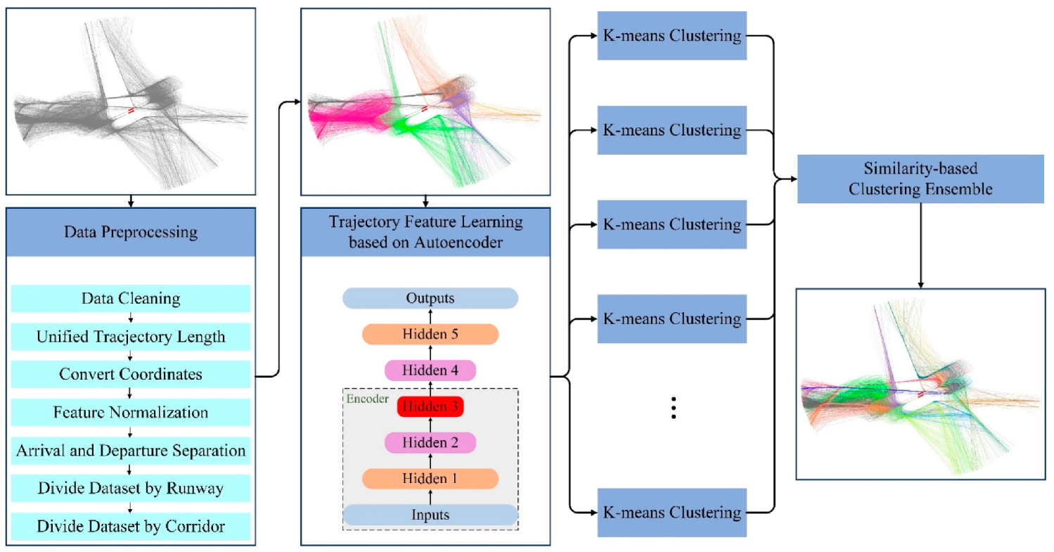
To solve the bottleneck problem faced by a single clustering algorithm in improving the clustering accuracy of aircraft trajectories, a clustering ensemble method of aircraft trajectory based on a similarity matrix is proposed in this paper. The implementation process of this method is shown in Figure 1. (1) Preprocess the data, including data cleaning, unifying trajectory lengths, transforming coordinates, feature normalization, separation of arrivals and departures, and dividing the dataset by runways and corridors. (2) Construct the derived property of angle empirically. (3) Use the stacked autoencoder to learn features that can efficiently represent trajectories. (4) Use the processed data obtained above as the input of each K-means basis cluster to acquire multiple clustering results. (5) Adopt the similarity-based clustering ensemble method to obtain the corresponding similarity matrix according to the results of each basis cluster [23]. Use all similarity matrixes to obtain the consistent similarity matrix. Next, (6) Take the deformation of the consistent matrix as the distance matrix between trajectories, and use agglomerative hierarchical clustering to ensemble the results of each basis cluster on the distance matrix, obtaining the final ensembled clustering results.
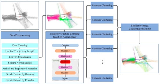
Figure 1.
The framework of the proposed method.
2.1. Data Preprocessing
Firstly, the quality analysis and cleaning of the trajectory data are carried out. Explore data for missing, duplicate, and mistyped waypoint data with quality analysis. If there is the duplicate and wrong type of waypoint data, delete it directly. Often, data will be partially missing. The reason for this situation is mostly due to the occasional abnormality of the equipment, which leads to the fact that the trajectory point data is not recorded for a certain period of time. Count the time interval between all adjacent trajectory points for each trajectory. According to the specific conditions of the data, for a certain trajectory, if the time interval between two consecutive points exceeds a certain threshold, the trajectory will be deleted. Second, unify the trajectory length. Count the number of trajectory points (trajectory length) for each trajectory. For the trajectory that is too short, delete it directly. Since the trajectory with too short a length cannot reflect the entire landing or take-off process of the aircraft in the terminal area, it is not beneficial to the subsequent clustering. On this basis, in order to use Euclidean distance to measure the similarity between trajectories, all trajectories are sampled to the same length by sampling. This is because Euclidean distance requires component correspondence. Of course, researchers can also choose the here methods to measure the similarity between trajectories without forcing the trajectories to have the same length [27,28].
In order to more intuitively reflect the trajectory position centered on the airport, the latitude and longitude coordinates in the data are converted into ENU (East-North-Up) Cartesian coordinate system with the center of the airport as the origin. Then, the values of all features are mapped to between 0 and 1 using the maximum and minimum normalization method, so as to prevent the problem that the value of a feature is generally large/small and the influence of the feature is too large/small. Due to the completely different operating modes of the incoming and outgoing flights, take-off and landing separation are performed on the trajectory. On this basis, in order to prevent the problem of uncontrollable results in the clustering process, the data set is divided into runways and corridors. When dividing the dataset by runway, trajectory points that fall on the runway are not considered. For the landing trajectory, calculate the distance between its last track point and each runway endpoint, and the runway represented by the nearest runway endpoint is the runway to which the track belongs. For a takeoff track, calculate the distance from its first track point to each runway endpoint. Next, divide the data set according to the corridors. For the landing trajectory, calculate the distance between its first trajectory point and each corridor, and the nearest corridor is the corridor to which it belongs. For the takeoff trajectory, calculate the distance between its last trajectory point and each corridor entrance.
It should be noted that the above data preprocessing steps do not take a long time. Since it mainly includes a simple data cleaning and data set division. Data set division also only needs to calculate the Euclidean distance between points, and the computational complexity is relatively low.
2.2. Derived Attribute Construction
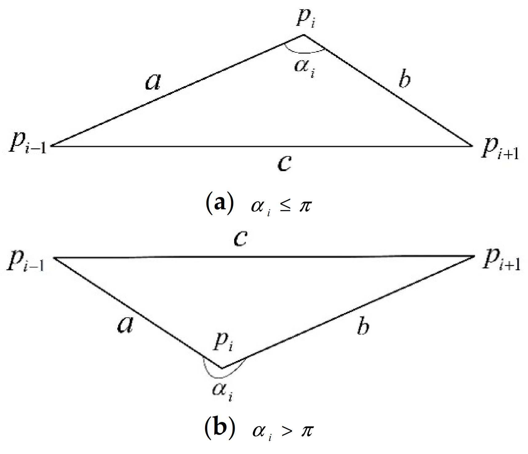
Since the shape feature of the trajectory cannot be reflected by its three-dimensional spatial position and heading features, to express the shape information of the trajectory, we construct an angle feature, denoted as . For a trajectory containing points, the angle value of each trajectory point is represented by the counterclockwise angle between the two line segments formed by points , and , where and are the two points immediately before and after the point . (Except for its first point and last point .). The calculation method of is shown in formula (1). Each symbol in the formula (1) can be represented in Figure 2.
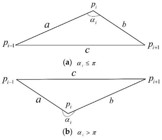
Figure 2.
Schematic diagram of angles.
In formula (1), represents the length of the horizontal line connecting the trajectory point and the immediately preceding trajectory point , represents the length of the horizontal line connecting the trajectory point and the immediately following trajectory point , represents the length of the horizontal line connecting the two trajectory points and before and after the trajectory point.
It should be noted that there is no point before the first point of the trajectory and there is no point after the last point . So for the angle values of and , the angle values of the next point of and the previous point of are used as the angle values of and , respectively.
2.3. Trajectory Feature Learning Based on the Stacked Autoencoder
Clustering analysis needs to use a large amount of historical trajectory data to make the results more regular and convincing, which leads to a larger length of data. In addition, the essence of the trajectory is a time series. If the entire trajectory is used as the clustering object, it is generally necessary to expand it into a row vector according to the time sequence during processing. Assuming that a trajectory has 90 points, and each trajectory point has only three spatial position features, then its dimensions also have as many as 270 dimensions. If a trajectory has more features and points, it will also have a larger dimension. This will seriously affect computational efficiency. At the same time, if there are too many trajectory points, redundant information may exist, or there may be a certain pattern, so it is unnecessary to use too many dimensions to represent a trajectory. Therefore, to improve the computational efficiency, we perform feature extraction and dimensionality reduction on the trajectory data.
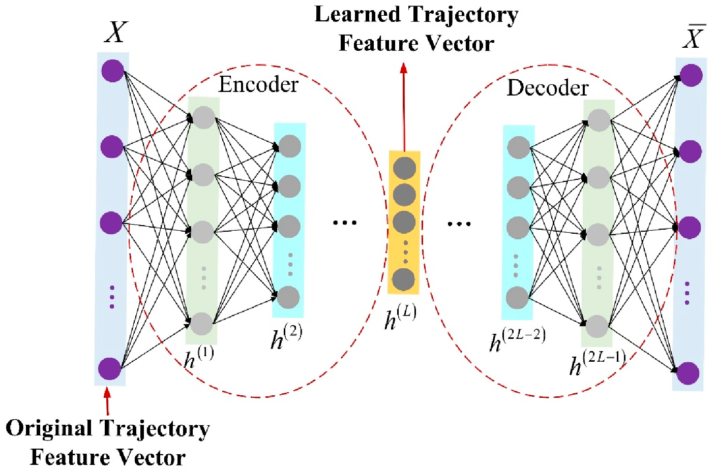
An autoencoder is an artificial neural network that learns to efficiently represent input data through unsupervised learning. Its goal is to restore the original input data with as little loss as possible. This coincides with our needs. A simple autoencoder refers to a neural network with only one input layer, one hidden layer, and one output layer [29]. However, the neural network has the same number of neurons in the input and output layers to try to reconstruct the input. The autoencoder network does not need data labels but uses the difference between the input and output to guide the network for training to find the optimal network parameters, so its objective function is shown in Equation (1). Therefore, it is a kind of unsupervised learning [30]. All types of autoencoders usually contain two parts, one is the encoder, which is the layer-by-layer learning from the input layer to the hidden layer, which learns to turn the input into an internal representation. The other is the decoder, which is layer-by-layer learning from the hidden layer to the output layer, which learns to reconstruct the input using the internal representation.
Since a simple autoencoder contains only one hidden layer, it may not be sufficient in some complex cases. Therefore, multi-layer autoencoders with multiple hidden layers called stacked autoencoders appeared. It can learn more complex encoded representations. In this paper, the stacked autoencoder is used for trajectory feature learning, and each trajectory is processed into a row vector in time sequence and input into the stacked autoencoder network. The stacked autoencoder takes the output of the hidden layer of its previous autoencoder as the input of its subsequent autoencoder, and the process can be represented in Figure 3. After integrating the individual autoencoders, the network structure of the stacked autoencoder is symmetric about the middle hidden layer. The network structure of a stacked autoencoder with hidden layers is shown in Figure 4. In practical applications, the output of the hidden layer of the last autoencoder is usually used, that is, the output of the middle hidden layer of the entire stacked autoencoder network.
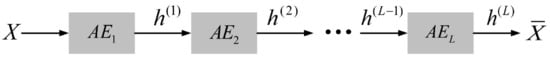
Figure 3.
Schematic diagram of the principle of stacked autoencoders with L autoencoders.
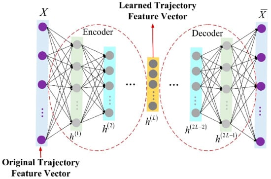
Figure 4.
Schematic diagram of the network structure of the stacked autoencoder.
The practice has shown that too many hidden layers can also cause the stacked autoencoder to fail to learn useful features. In application, the network hyperparameters including the number of hidden layers are generally set according to the training data and training effects and through a large number of experiments. According to the dimension and length of the specific data, set each parameter to be a set within a certain value range, and then randomly select N from all possible network hyperparameter combinations. Then, the parameter configuration that minimizes the objective function value is the optimal parameter, which is the network hyperparameter we are looking for.
2.4. Trajectory Clustering Ensemble Based on the Similarity Matrix
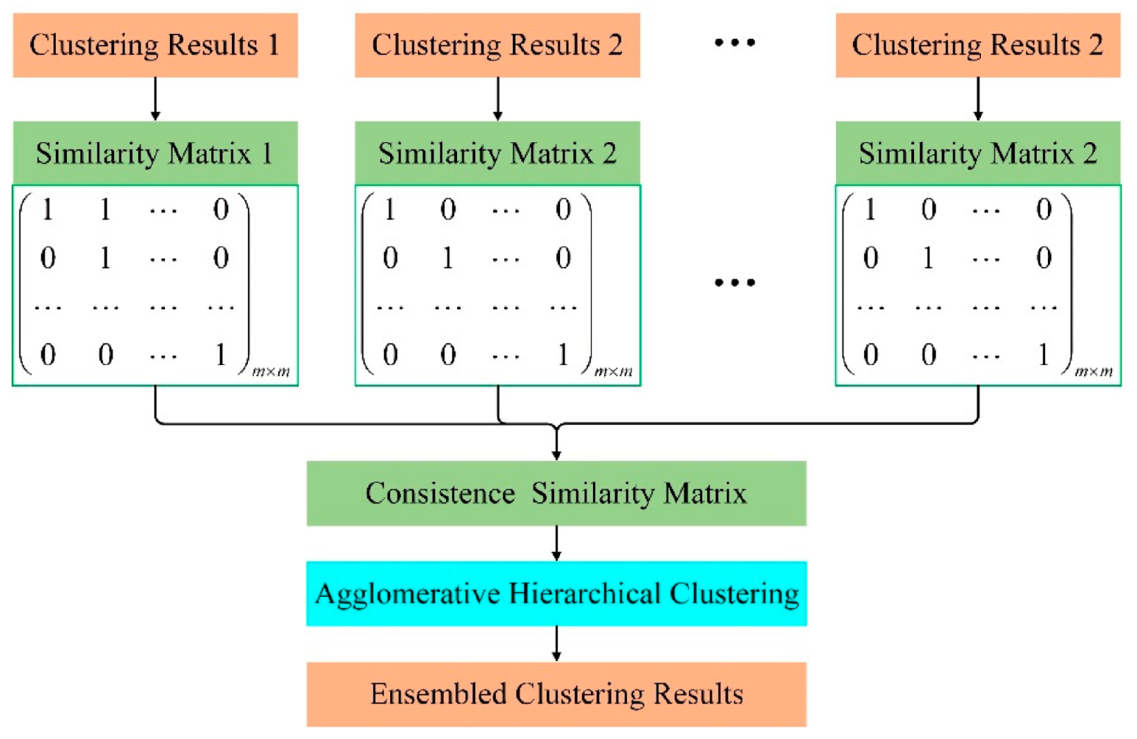
At present, most trajectory clustering uses a single clustering method for clustering. When other processing remains unchanged, it is difficult to improve the clustering effect by using a single clustering method. If we want to improve the clustering effect on this basis, we can use multiple different clustering methods to generate multiple clustering results, and then combine these clustering results to make full use of the information contained in each result to obtain cluster ensemble results of higher quality [21]. This approach is called cluster ensemble. The key and difficult problem of clustering ensemble is how to properly express and combine the results of each basis cluster. Clustering ensembles can be roughly classified into similarity-based methods, graph-based methods, relabeling-based methods, and transformation-based methods [21,22,31]. Among them, the basic idea of the similarity-based method is to use the clustering results of multiple basis clusters to obtain a consistent similarity matrix and use the consistent similarity matrix to express the connection and information between each basis cluster. The method is easy to implement and aggregate, and can be used to ensemble multiple clustering methods.
Therefore, this paper adopts the clustering ensemble method based on similarity to ensemble the clustering results of multiple K-means basis clusters. When integrating the individual clustering results, the data clustering method based on evidence accumulation was proposed by Fred et al. [23] was introduced. According to the results of each basis cluster, the corresponding similarity matrix is obtained, and these similarity matrices are used to generate a consistent similarity matrix, and then the deformation of the consistent similarity matrix is used as the distance matrix between trajectories. Under a certain aggregation threshold level, using agglomerative hierarchical clustering to obtain ensemble clustering results. This process can be represented in Figure 5. The idea of agglomerative hierarchical clustering is to first treat each sample as a cluster, and then repeatedly merge the two closest clusters until the iteration termination condition is satisfied or all samples are in one cluster [32]. There are single connections, full connections, and average connections for calculating the distance between clusters [33].
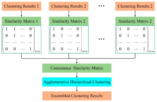
Figure 5.
Flow chart of clustering ensemble based on a similarity matrix.
The specific implementation steps of the trajectory clustering ensemble method based on similarity in this paper are as follows:
Assuming that the input dataset has trajectories, each trajectory is denoted as . Then the dataset is denoted as .
Step 1: Run the K-means algorithm times on the data set , and each time you can select the same or the different number of parameter clusters , thereby obtaining clustering results . where is a -dimensional vector , and each element of represents the clustering label for each trajectory.
Step 2: Obtain the corresponding similarity matrix from each clustering result . A consistent similarity matrix is obtained from these similarity matrices. The rules for generating the similarity matrix according to the result of the basis cluster are as follows: if , it means that the clustering categories of the trajectories and are the same, that is, they are in the same cluster, then the element of the similarity matrix , otherwise . So each similarity matrix is a binary matrix whose each element indicates whether each pair of trajectories occurs in the same cluster. The consistent similarity matrix is equal to the average of these similarity matrices, that is, , where the value of every element of is between 0 and 1, indicating that trajectories and have probability of appearing in the same cluster in the results of the basis clusters. The idea of generating each element in the consensus similarity matrix here is similar to the principle of majority voting.
Step 3: Take as the distance between trajectories and , that is, take as the distance matrix, and use the single-connected agglomerative hierarchical clustering algorithm () as the consistent cluster to find consistent clusters at the threshold level [23]. Since the value of each element of the matrix is between 0 and 1, every element of the matrix also has a value between 0 and 1. The specific meaning of the threshold is: when the distance between the two closest clusters is less than , the two clusters are merged, otherwise they are not merged. The value range of is between 0 and 1, and its empirical value is 0.5.
To sum up, there are three parameters that need to be adjusted in the trajectory clustering ensemble method based on similarity in this paper, one is the number of basis clusters, one is the number of clusters of each basis cluster, and one is the connection threshold . The pseudocode of this method is shown in Algorithm 1. If you want to use other basis clusters, the basis clusters can also be replaced by other clustering methods. The method of adjusting the parameters adopts the method mentioned at the end of Section 2.1, that is, given the optional value of each parameter, and then randomly selects N from all parameter combinations for the experiment, and this N is also the number of experiments. The parameter combination that minimizes the sum of squared errors within the cluster SSE (see Section 3.2 for the clustering evaluation index SSE) is the optimal parameter configuration.
| Algorithm 1. Clustering ensemble algorithm based on similarity |
| Inputs: (1) Data Set ; (2) The number of basis clusters, ; (3) Number of clusters per basis cluster, ; (4) Basis Cluster, ; (5) Consistent Cluster, ; (6) The threshold level, ; Outputs: Cluster ensemble results, ; Algorithm:
|
3. Experimental Results and Discussion
In this section, the data set used is briefly explained in Section 3.1, and the results of preprocessing the data set are introduced. Second, in Section 3.2, the three evaluation indexes used in this paper to evaluate the clustering results are introduced. On this basis, the experimental results are given in Section 3.3. Finally, Section 3.4 discusses and analyzes the parameters used in the method.
3.1. Data Preprocessing
The dataset used in this paper comes from the secondary radar data of Nanjing Lukou International Airport (ICAO four-character code: ZSNJ). The data range is the trajectory within a radius of 70 km centered on the airport. The time span of the dataset is from 20 July to 18 August 2019 (30 days in total), with a total of 14,305 trajectories. The scanning period of the secondary radar is 4 s, that is, the trajectory points are recorded every 4 s. The information for each trajectory point includes time, flight number, longitude, latitude, altitude, heading, speed, rate of descent, etc. In clustering, we use the first five attributes and also use the angle feature constructed in Section 2.2.
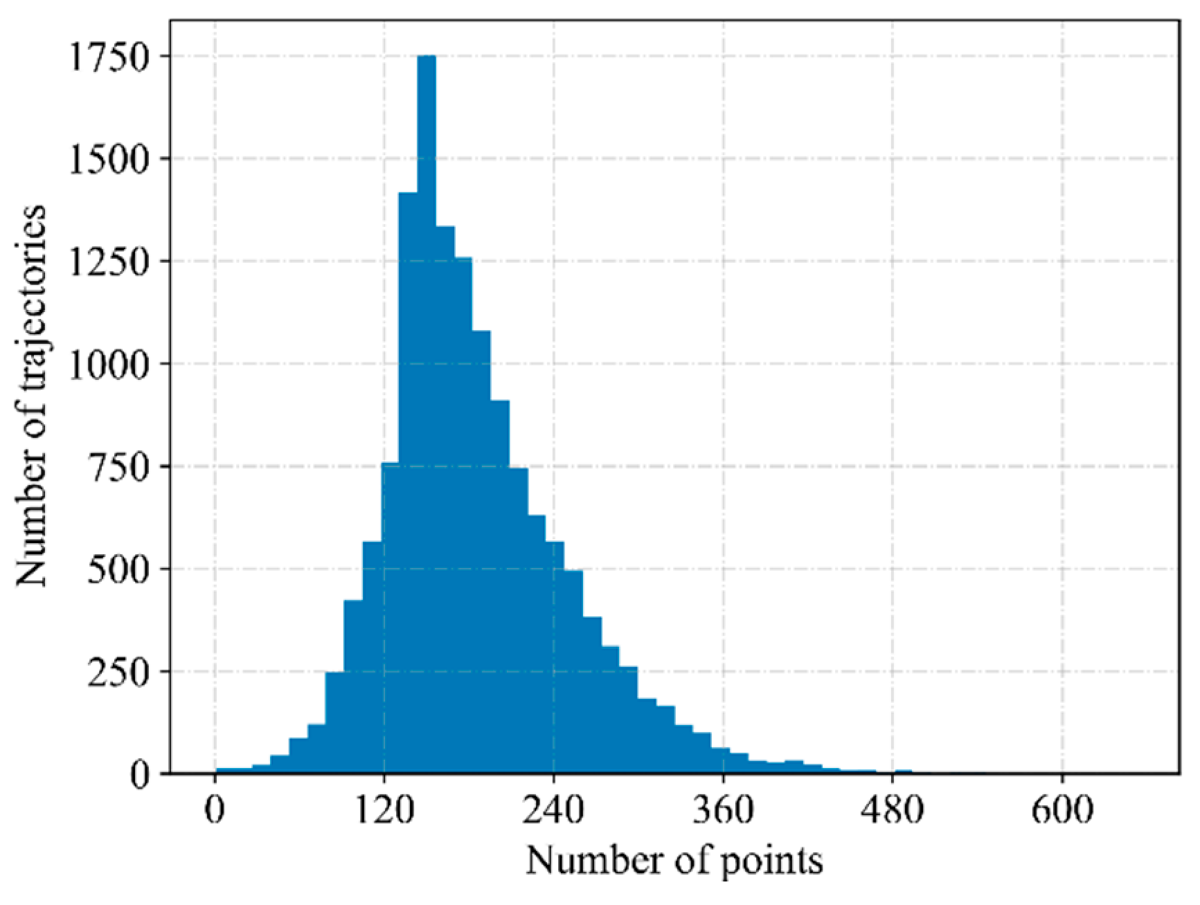
The dataset used in this paper is preprocessed according to the data preprocessing method proposed in Section 2.1. Delete trajectories with a time interval of more than 90 s between two consecutive points. Count the number of trajectory points (trajectory length) of each trajectory, as shown in Figure 6. For trajectories whose length is less than 88, delete them directly. On this basis, all trajectories are sampled to 88 trajectory points.

Figure 6.
Histogram of trajectory length.
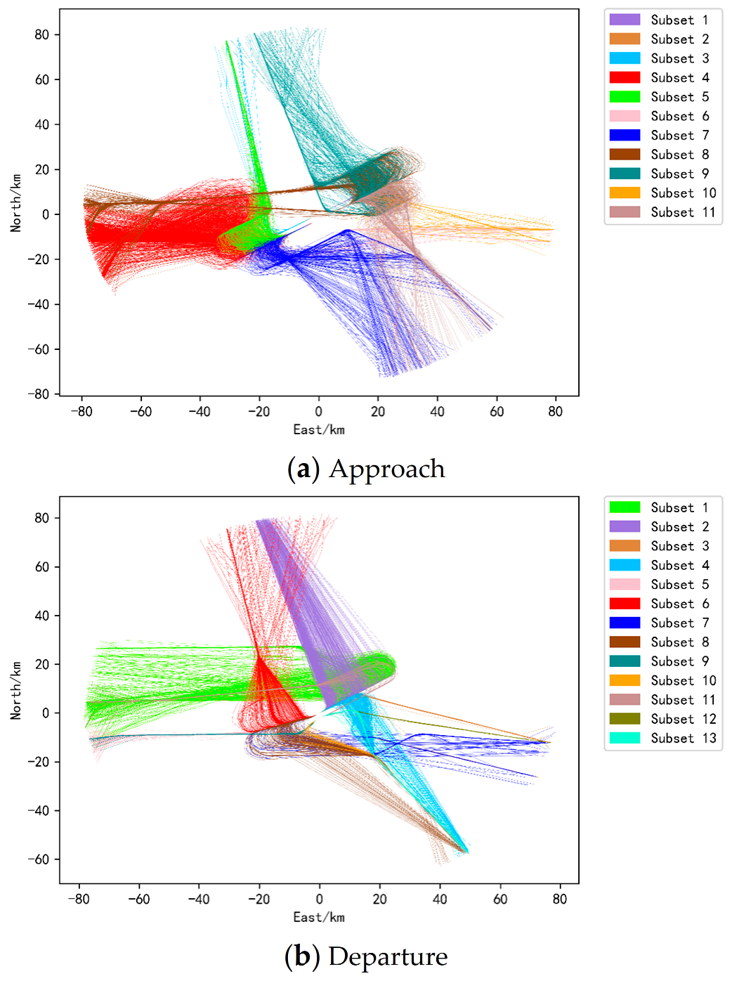
ZSNJ has 2 runways (4 directions), 5 arrival corridors, and 4 departure corridors. Then, after dividing the data set according to runways and corridors, the arrival and departure trajectory data sets should be divided into 20 and 16 small data sets, respectively. However, there are no or few trajectories at a certain corridor of some runways, so the arrival and departure trajectories are finally divided into 11 and 13 small datasets, respectively, as shown in Figure 7. Trajectories in the same color in the figure indicate that they belong to the same runway and corridor. The basic situation of each small sub-data set after division is further displayed in Table 1, including the serial number of each sub-data set (corresponding to Figure 7), the runway and corridor to which it belongs, the number of trajectories it has, and the number of clusters it is divided into (The number of clusters is obtained after clustering. Since the experiment has been carried out, it is shown here.). Next, we construct angular features according to the angular attribute construction method proposed in Section 2.2 and then construct a stacked autoencoder network to extract the main features of the trajectory. Using the network hyperparameter setting method mentioned at the end of Section 2.3, 400 experiments were designed to select the optimal hyperparameters. According to the dimension and length of the data, the number of hidden layers is set to {1, 3, 5, 7, 9}, and the number of neurons in the hidden layer is {330, 220, 110, 55, 11}. Finally, it is determined that the number of hidden layers of the network is 5, and the number of neurons in each layer is {110, 55, 11, 55, 110}.

Figure 7.
The trajectories after the division of the runway and the corridor.

Table 1.
Basic information of each sub-dataset.
3.2. Evaluation Index of Clustering Results
Suppose a dataset containing trajectories is clustered into classes, where represents the -th cluster, represents the center trajectory of the -th cluster, and represents a trajectory in the dataset . To clarify the quality of the clustering results, this paper adopts three clustering results evaluation indicators, namely the intra-cluster error variance SSE, the silhouette coefficient SC, and CH indicators.
The intra-cluster error variance SSE calculates the sum of the Euclidean distances of all trajectories and their respective center trajectories, measuring the compactness of the cluster.
The silhouette coefficient SC measures the quality of clustering from the perspective of intra-cluster compactness and inter-cluster separation. Generally, the mean of all trajectory silhouette coefficients is used as the overall silhouette coefficient, and the overall silhouette coefficient is used to measure the overall quality of the clustering results. The silhouette coefficient has a value between −1 and 1. The closer its value is to 1, the more reasonable the clustering of the trajectory ; the closer the value is to −1, the more the trajectory should be clustered into other clusters; the value is close to 0, indicating that the trajectory is closer to the boundary of the two clusters. For any trajectory , its silhouette coefficient SC is defined as:
In the formula (4), is the average distance between the trajectory and other trajectories in the cluster to which it belongs, reflecting the compactness of the cluster to which belongs. The smaller the value, the more compact it is. is the minimum value of the average distance from to all other clusters, reflecting the degree of separation from other clusters. The larger the value, the greater the degree of separation. Assuming that the trajectory belongs to the -th cluster, the calculation formula of is shown in formula (5), which represents the number of trajectories contained in the -th cluster.
Another clustering result evaluation index, Calinski-Harabaz (CH), uses the ratio of between-class variance and within-class variance to measure the quality of clustering results, as shown in formula (6). In formula (6), is the mean of all the trajectories in the trajectory data set , that is, the center trajectory of the entire data set. The numerator of formula (5) calculates the ratio of the sum of the squares of the distances between the center trajectory of each cluster and the center trajectory of the entire dataset to , which represents the degree of separation between clusters. The denominator calculates the ratio of the sum of the squares of the distances between all trajectories and the center trajectory of their respective clusters to , which represents the compactness within the class. Obviously, if the numerator is larger and the denominator is smaller, the larger the score, the better the clustering.
3.3. Experimental Results
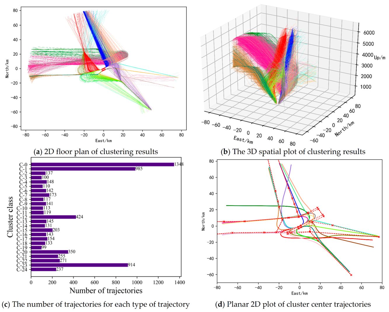
A total of 24 types of landing trajectories and 25 types of take-off trajectories were obtained by the clustering ensemble method based on similarity. By simply averaging the points to calculate the average value of each cluster of trajectories, 24 landing center trajectories and 25 take-off center trajectories were correspondingly obtained. The results are shown in Figure 8 and Figure 9. The calculation of the central trajectory here can also adopt the calculation method of the average route that can tolerate outliers proposed by Pasi Fränti et al. [34].
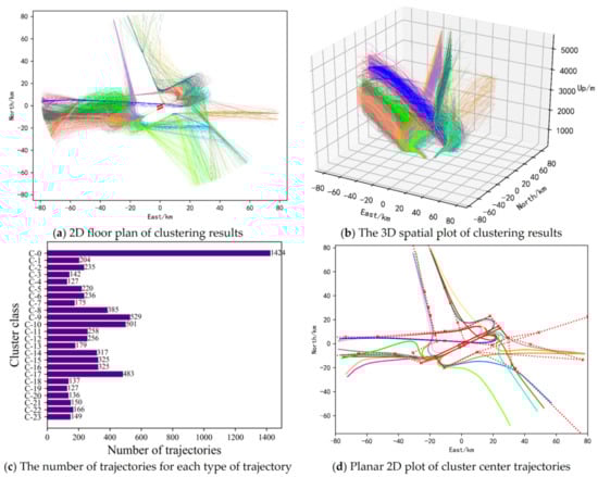
Figure 8.
Clustering results of Landing trajectories.

Figure 9.
Clustering results of takeoff trajectories.
In Figure 8, the clustering results of all landing trajectories in the terminal airspace of Nanjing Lukou Airport can be seen intuitively. Among them, Figure 8a is a two-dimensional floor plan of the clustering results of all landing trajectories. Trajectories with the same color in Figure 8a represent trajectories belonging to the same cluster. Flight trajectories of the same cluster are relatively similar and can be considered to be the same traffic flow and have the same flight pattern. Combined with Figure 8b, the spatial distribution of each traffic flow of the terminal area airspace approach trajectory can be obtained. By counting the number of trajectories contained in each cluster trajectories, as shown in Figure 8c, the traffic density of each approaching traffic flow can be obtained. From the information obtained above, the usage of each sector in the terminal airspace of the airport can be known, so as to provide a direct basis for the optimization of sector division. In addition, from Figure 8c, it can be found that the number of trajectories contained in a few clusters is significantly more than the number of trajectories contained in other clusters. By counting the number of trajectories in the top three clusters, it is found that these trajectories all land on runways 07 and 25. Therefore, it can be known that runways 07 and 25 are the main runways for landing. The central trajectories of each cluster trajectories are shown in Figure 8d. The red dotted line in Figure 8d represents the standard approach flight procedure, and the solid lines in other colors represent the central trajectory, which can also be considered as the prevailing flight trajectory of the aircraft in the terminal area. As can be seen from Figure 8d, most of the center trajectories are in good agreement with the standard flight procedure, but some central trajectories have a large deviation from the standard flight procedure. The reason may be the controller’s control habits, radar guidance, flow control, special weather, etc., resulting in a flight pattern that is different from the standard flight procedure. This can provide a strong reference for us to formulate and modify standard flight procedures, and it is also the significance of trajectory clustering. It can only use the existing historical data to obtain the inherent laws of aircraft operation, providing important technical support for the safe and orderly operation of air traffic.
The clustering results of all takeoff trajectories in the terminal airspace of Nanjing Lukou Airport are shown in Figure 9. Combining the two-dimensional plane map (Figure 9a) and the three-dimensional spatial map (Figure 9b) of the clustering results, we can understand the spatial distribution of various take-off trajectories. Comparing it with the various landing trajectories, it can be found that the take-off trajectory is more regular. Counting the number of trajectories in the top three classes, it is found that these trajectories all take off from runways 06 and 24. Therefore, it can be known that runways 06 and 24 are the main runways for takeoff. Combining with Figure 9a–c, we can acquire the current usage of each sector in the airspace and the distribution of each traffic flow of aircraft taking off, which has direct guiding significance for the reasonable division of airspace sectors and the control of sector traffic flow. In addition, the center trajectories obtained by cluster analysis of flight trajectories can be used to provide a reference for the revision of standard flight procedures. The center trajectories of each cluster of the take-off trajectory are shown in Figure 9d. Comparing the trajectories of the center of arrival and departure horizontally, we can see that the agreement between the prevailing flight trajectories of departing aircraft and the standard departure flight procedures is higher than that of the prevailing flight trajectories of arriving aircraft and the standard arrival flight procedures. To a certain extent, it confirms the conclusion that the take-off trajectory obtained above is more regular than the landing trajectory.
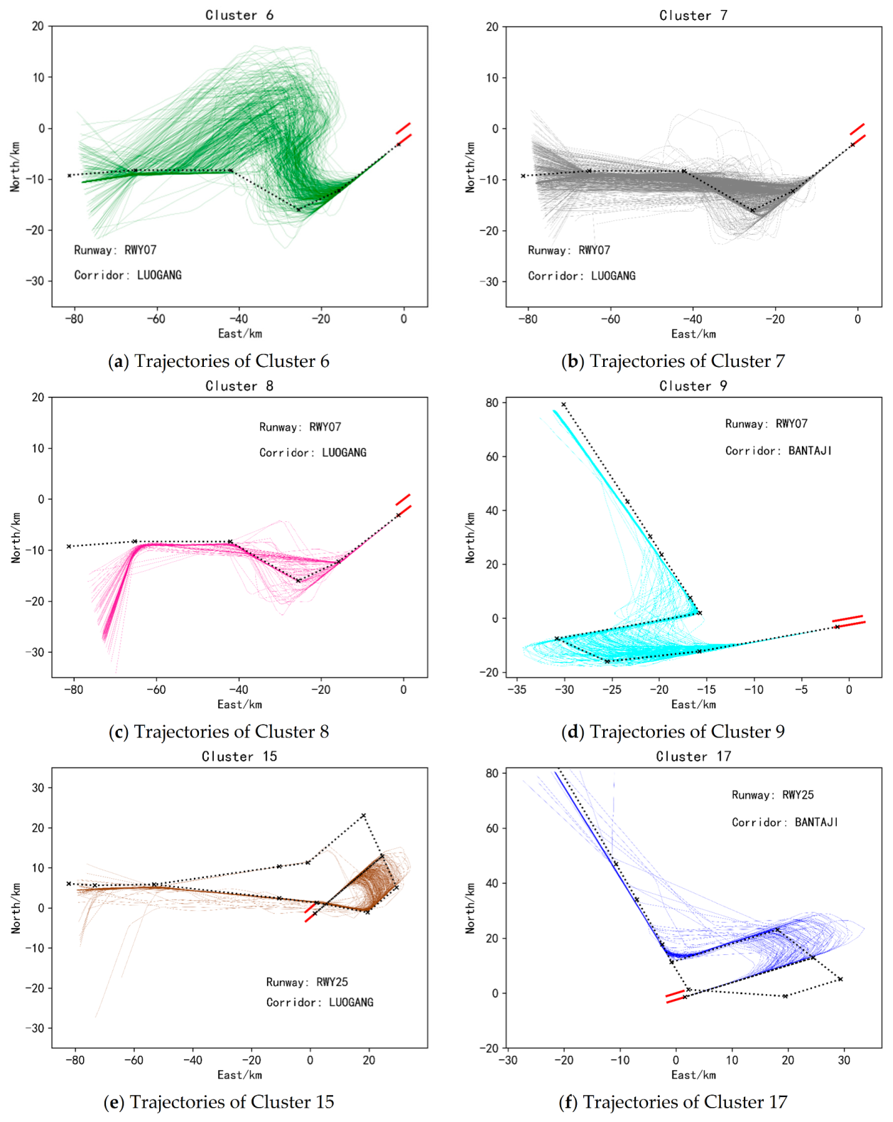
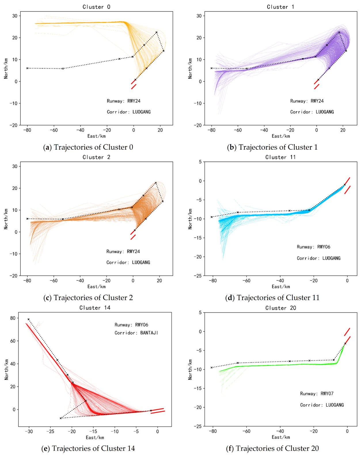
To display the clustering results more intuitively, the two-dimensional plan views of 6 types of approach trajectories and 6 types of departure trajectories are selected for display, as shown in Figure 10 and Figure 11. Each picture in Figure 10 and Figure 11 shows that each type of trajectory belongs to a certain corridor and runway. The black dotted line in Figure 10 represents the standard approach flight procedure plus the standard approach procedure through the corresponding corridor and runway. The black dashed lines in Figure 11 represent standard departure flight procedures through the corresponding corridor openings and runways. Among them, there are two standard flight procedures in Figure 10d,e, indicating that there are two standard flight procedures for passing through the corridor and the runway. It can be seen from Figure 10 and Figure 11 that the similarity of trajectories between various clusters is small, while the similarity of trajectories within the same cluster is large, which can preliminarily show the effectiveness of the method in this paper. In addition, comparing the various trajectories with the standard flight procedures they should follow, it can be found that some trajectories are not strictly following the standard flight procedures, and are quite different from the standard flight procedures, as shown in Figure 10c and Figure 11a. This is also the significance of clustering massive trajectory data, which is to discover the information contained in the actual historical operation data of the aircraft. And then we can compare it with the prior knowledge to find the differences and similarities, to provide the basis for future planning for ATS stakeholders.
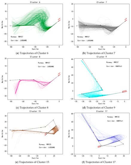
Figure 10.
Two-dimensional plan view of some landing clusters.
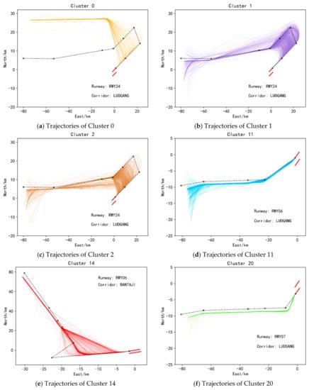
Figure 11.
Two-dimensional plan view of some takeoff clusters.
3.4. Parameter Discussion
In order to verify the superiority of the clustering ensemble method, we used the single K-means clustering algorithm [7] to cluster the dataset used in this paper and calculated the clustering evaluation index value of the ensembled clustering results and the single clustering results and the time taken for both, as shown in Table 2 and Table 3. It can be seen from Table 2 and Table 3 that the clustering evaluation index values of the ensembled clustering results are better than the single clustering results. However, ensemble clustering took 10 times more time than single clustering. So, the cost of ensemble is that it needs more time. However, since trajectory clustering is widely used, for example, it can provide a reference for the revision of standard flight procedures, so it does not need to be fast, but requires more accurate clustering results. Ensemble clustering just satisfies this requirement because of its relatively high accuracy.
Table 2.
Comparison index values of clustering results of ensembled K-means and single K-means of landings.
Table 3.
Comparison index values of clustering results of ensembled K-means and single K-means of takeoffs.
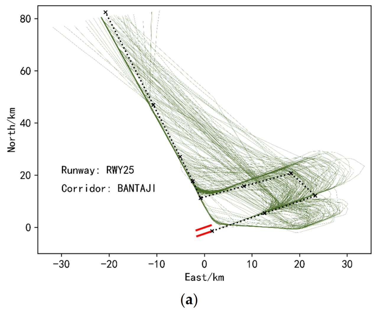
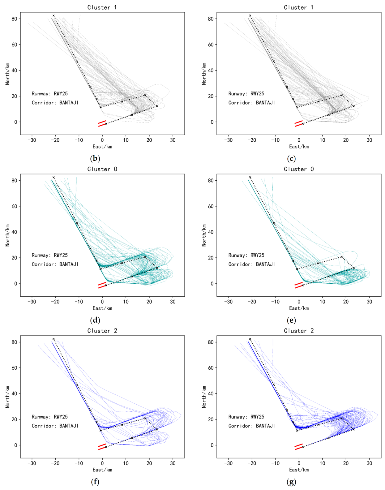
In addition, we also found that when faced with some inherently compact trajectory data, single K-means showed poor results, while ensemble K-means still performed well, as shown in Figure 12. This figure is the visualization of the single K-means clustering results and the ensembled K-means clustering results of the trajectory data from the corridor entrance BANTAJI entering the terminal airspace of Nanjing Lukou Airport and landing on runway 25. Figure 12a is an overall visualization of this sub-dataset, and it can be seen that the dataset itself is relatively compact. The results obtained by clustering this dataset using a single K-means are shown in Figure 12b,d,f. From these three sub-figures, it can be found that a single K-means is indeed not effective for this type of dataset Clustering, because the trajectories in Figure 12d,f not only have a small similarity between intra-class trajectories, but also a large similarity between classes, which is seriously inconsistent with the goal of clustering. However, it can be solved if the similarity-based ensemble clustering algorithm proposed in this paper is used, as shown in Figure 12c,e,g. This also shows that the ensemble clustering method proposed in this paper can identify more diverse data structures and has better generalization ability.

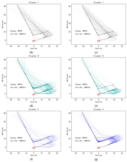
Figure 12.
(a) Overall visualization of trajectories of runway25, corridor BANTAJI. (b) Cluster 1 trajectories under the single K-means clustering method. (c) Cluster 1 trajectories under ensemble K-means clustering method. (d) Cluster 0 trajectories under the single K-means clustering method. (e) Cluster 0 trajectories under ensemble K-means clustering method. (f) Cluster 2 trajectories under the single K-means clustering method. (g) Cluster 2 trajectories under ensemble K-means clustering method. Clustering results of landing trajectories of the BANTAJI corridor and Runway 25 under the single K-means clustering method and ensemble K-means method.
When using the similarity-based integrated K-means clustering algorithm, it is necessary to comprehensively adjust the threshold, the number of base clusterers and the K value of each base clusterer according to the parameter selection method mentioned at the end of Section 3.3 to obtain the best clustering effect.
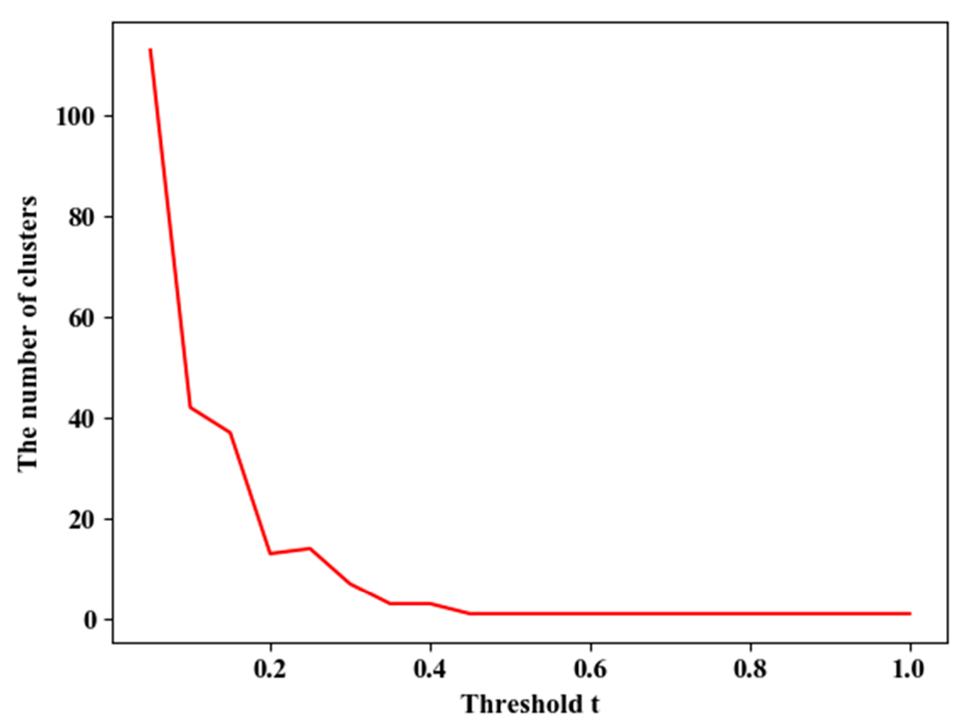
The meaning of the threshold is that when the distance between the two clusters is less than , the two clusters are merged. If the threshold is larger, the cost of the connection is smaller, that is, it is easier to connect the two clusters, so the number of the final clusters is less. On the contrary, more clusters are formed. Taking the dataset of Runway 25 and the BANTAJI corridor of Nanjing Lukou Airport as an example, different thresholds are selected, and the methods of a single connection, full connection, and average connection are used, respectively, in the ensemble. The change in the number of clusters is shown in Figure 13. As can be seen from the Figure 13, the number of clusters decreases with the increase of the threshold and decreases faster when the threshold is smaller. When the threshold is larger, the change of the number of clusters is smaller. And when the threshold reaches 1, the number of clusters also becomes 1. Therefore, when selecting the range of the threshold , more values of could be selected when the threshold is smaller.

Figure 13.
Variation of the number of categories K with the threshold under each connection method.
As mentioned in Section 2.4, the value of K of each basis cluster can be fixed or not, that is, the same or different K can be selected each time when a single K-means algorithm is executed. However, in the actual process of using the algorithm, generally choosing different K values will acquire better results. The result obtained by ensemble 20 basis clusters and the value of K of each base cluster is different is shown in Figure 12c,e,g (The values of K are {2, 3, 4, 5, 6, 7, 8, 9, 3, 4, 5, 6, 7, 8, 9, 10, 3, 4, 5, 3}. And the threshold t has a value of 0.35.). The clustering result obtained by integrating 20 basis clusters and the K value of each basis cluster is selected as 3 (The threshold is 0.45.) is similar to the clustering result obtained by single K-means, as shown in Figure 12b,d,f. The reason is that the clustering results that can be obtained with different K values are more diverse, and the useful information of each basis cluster will be ensembled during the clustering ensemble, to obtain higher-quality clustering ensemble results.
Regarding the number of basis clusters, it is generally necessary to select multiple basis clusters, but the number of basis clusters should not be too many to prevent the problem of low computational efficiency.
4. Conclusions
Massive trajectory data contains inherent information such as the prevailing flight patterns of aircraft. At present, the most efficient way to mine this information is to perform cluster analysis on trajectories. However, since most of the trajectory clustering algorithms used in the current are the single clustering algorithm, it is difficult to improve the clustering effect by this method. Therefore, this paper introduces a trajectory clustering ensemble method based on a similarity matrix. Firstly, in the data preprocessing stage, the trajectory dataset is divided according to the runway and corridor to which each trajectory belongs. To make full use of the information in the trajectory data, an angular feature that can express the shape of the trajectory is also constructed. Secondly, to reduce the data dimension, the stacked autoencoding network is used to perform feature learning on each dataset, and data that can represent the original trajectory with fewer features is obtained. Next, each dataset is clustered using multiple K-means basis clusters. Finally, the clustering ensemble method based on a similarity matrix is adopted to ensemble the results of each basis cluster. Through the experimental verification, it is found that compared with the single clustering algorithm, higher quality and more robust clustering results can be obtained by using the trajectory clustering ensemble method based on the similarity matrix proposed in this paper. The method does not depend on a specific dataset and can handle a wider variety of dataset types, so it can be used in other terminal areas and generalized to enroute flight scenarios. In the future, we can continue to study the ensemble of different clustering methods to explore more efficient ensemble methods.
Author Contributions
Conceptualization, X.C. and W.Z.; methodology, X.C. and W.Z.; investigation, X.C. and X.T.; data curation, W.Z. and X.T.; supervision, W.Z.; validation, W.Z. and X.T.; writing—original draft preparation, X.C. and W.Z.; writing—review and editing, X.C and X.T. All authors have read and agreed to the published version of the manuscript.
Funding
This work was supported by State Key Laboratory of Air Traffic Management System and Technology [No: SKLATM202007]; National Natural Science Foundation of China [No. 62076126].
Institutional Review Board Statement
Not applicable.
Informed Consent Statement
Not applicable.
Data Availability Statement
This study did not report any data.
Acknowledgments
We would like to thank the National Air Traffic Control Flight Flow Management Technology Key Laboratory of Nanjing University of Aeronautics and Astronautics for providing the ADS-B data used in the model tests described in this paper.
Conflicts of Interest
The authors declare no conflict of interest.
References
- Le, T.H.; Tran, P.N.; Pham, D.T.; Schultz, M.; Alam, S. Short-Term trajectory prediction using generative machine learning methods. In Proceedings of the ICRAT 2020 Conference, Tampa, FL, USA, 15 September 2020. [Google Scholar]
- Gallego, C.E.V.; Comendador, V.F.G.; Nieto, F.J.S.; Imaz, G.O.; Valdés, R.M.A. Analysis of air traffic control operational impact on aircraft vertical profiles supported by machine learning. Transp. Res. Part C Emerg. Technol. 2018, 95, 883–903. [Google Scholar] [CrossRef]
- Zhong, H.; Liu, H.; Qi, G. Analysis of Terminal Area Airspace Operation Status Based on Trajectory Characteristic Point Clustering. IEEE Access 2021, 9, 16642–16648. [Google Scholar] [CrossRef]
- Han, P.; Wang, W.; Shi, Q.; Yue, J. A combined online-learning model with K-means clustering and GRU neural networks for trajectory prediction. Ad Hoc Netw. 2021, 117, 102476. [Google Scholar] [CrossRef]
- Jiang, S.Y.; Luo, X.; He, L. Research on method of trajectory prediction in aircraft flight based on aircraft performance and historical trajectory data. Math. Probl. Eng. 2021, 2021, 6688213. [Google Scholar] [CrossRef]
- Ayhan, S.; Samet, H. DICLERGE: Divide-Cluster-Merge Framework for Clustering Aircraft Trajectories. In Proceedings of the 8th ACM SIGSPATIAL International Workshop on Computational Transportation Science, Seattle, WA, USA, 3 November 2015; pp. 7–14. [Google Scholar]
- Barratt, S.T.; Kochenderfer, M.J.; Boyd, S.P. Learning probabilistic trajectory models of aircraft in terminal airspace from position data. IEEE Trans. Intell. Transp. Syst. 2018, 20, 3536–3545. [Google Scholar] [CrossRef] [Green Version]
- Yang, Z.; Tang, R.; Chen, Y.; Wang, B. Spatial–Temporal Clustering and Optimization of Aircraft Descent and Approach Trajectories. Int. J. Aeronaut. Space Sci. 2021, 22, 1512–1523. [Google Scholar] [CrossRef]
- Chakrabarti, S.; Vela, A.E. Clustering Aircraft Trajectories According to Air Traffic Controllers’ Decisions. In Proceedings of the 2020 AIAA/IEEE 39th Digital Avionics Systems Conference (DASC), San Antonio, TX, USA, 11–15 October 2020; pp. 1–9. [Google Scholar]
- Kenefic, R.J. Trajectory Clustering Using Fréchet Distance and Minimum Description Length. J. Aerosp. Inf. Syst. 2014, 11, 512–524. [Google Scholar]
- Madar, S.; Puranik, T.G.; Mavris, D.N. Application of Trajectory Clustering for Aircraft Conflict Detection. In Proceedings of the 2021 IEEE/AIAA 40th Digital Avionics Systems Conference (DASC), San Antonio, TX, USA, 11–15 October 2021. [Google Scholar]
- Olive, X.; Basora, L. Identifying Anomalies in Past En-Route Trajectories with Clustering and Anomaly Detection Methods; ATM Seminar: Vienne, Austria, 2019. [Google Scholar]
- Gallego, C.E.V.; Comendador, V.F.G.; Nieto, F.J.S.; Martinez, M.G. Discussion On Density-Based Clustering Methods Applied for Automated Identification of Airspace Flows. In Proceedings of the 2018 IEEE/AIAA 37th Digital Avionics Systems Conference (DASC), London, UK, 23–27 September 2018; pp. 584–593. [Google Scholar]
- Tang, J.; Liu, L.; Wu, J.; Zhou, J.; Xiang, Y. Trajectory clustering method based on spatial-temporal properties for mobile social networks. J. Intell. Inf. Syst. 2021, 56, 73–95. [Google Scholar] [CrossRef]
- Salarpour, A.; Khotanlou, H. Direction-based similarity measure to trajectory clustering. IET Signal Processing 2019, 13, 70–76. [Google Scholar] [CrossRef]
- Zhang, D.; Lee, K.; Lee, I. Hierarchical trajectory clustering for spatio-temporal periodic pattern mining. Expert Syst. Appl. 2018, 92, 1–11. [Google Scholar] [CrossRef]
- Deng, C.; Kim, K.; Choi, H.C.; Hwang, I. Trajectory pattern identification for arrivals in vectored airspace. In Proceedings of the 2021 IEEE/AIAA 40th Digital Avionics Systems Conference (DASC), San Antonio, TX, USA, 3–7 October 2021. [Google Scholar]
- Zeng, W.; Xu, Z.; Cai, Z.; Chu, X.; Lu, X. Aircraft Trajectory Clustering in Terminal Airspace Based on Deep Autoencoder and Gaussian Mixture Model. Aerospace 2021, 8, 266. [Google Scholar] [CrossRef]
- Chen, L.; Zeng, W.; Yang, Z. An Aircraft Trajectory Anomaly Detection Method Based on Deep Mixture Density Network. Trans. Nanjing Univ. Aeronaut. Astronaut. 2021, 38, 840–851. [Google Scholar]
- Fern, X.Z.; Lin, W. Cluster ensemble selection. Stat. Anal. Data Min. ASA Data Sci. J. 2008, 1, 128–141. [Google Scholar] [CrossRef]
- Zhou, Z.-H. Ensemble Learning. In Machine learning; Springer: Berlin/Heidelburg, Germany, 2021; pp. 181–210. [Google Scholar]
- Fern, X.Z.; Brodley, C.E. Solving cluster ensemble problems by bipartite graph partitioning. In Proceedings of the Twenty-First International Conference on Machine Learning, Banff, AB, Canada, 4–8 July 2004. [Google Scholar]
- Fred, A.L.; Jain, A.K. Data clustering using evidence accumulation. In Proceedings of the 2002 International Conference on Pattern Recognition, Quebec City, QC, Canada, 11–15 August 2002. [Google Scholar]
- Topchy, A.P.; Law, M.H.; Jain, A.K.; Fred, A.L. Analysis of consensus partition in cluster ensemble. In Proceedings of the Fourth IEEE International Conference on Data Mining (ICDM’04), Brighton, UK, 1–4 November 2004. [Google Scholar]
- Olive, X.; Basora, L.; Viry, B.; Alligier, R. Deep Trajectory Clustering with Autoencoders. In Proceedings of the International Conference on Research in Air Transportation, online, 15 September 2020. [Google Scholar]
- Fränti, P. Efficiency of random swap clustering. J. Big Data 2018, 5, 13. [Google Scholar] [CrossRef]
- Müller, M. Dynamic time warping. In Information Retrieval for Music and Motion; Springer: Berlin/Heidelburg, Germany, 2007; pp. 69–84. [Google Scholar]
- Mariescu-Istodor, R.; Fränti, P. Grid-based method for GPS route analysis for retrieval. ACM Trans. Spat. Algorithms Syst. 2017, 3, 1–28. [Google Scholar] [CrossRef]
- Tschannen, M.; Bachem, O.; Lucic, M. Recent advances in autoencoder-based representation learning. arXiv 2018, arXiv:1812.05069. [Google Scholar] [CrossRef]
- Ng, A. Sparse autoencoder. CS294A Lect. Notes 2011, 72, 1–19. [Google Scholar]
- Iam-On, N.; Boongoen, T.; Garrett, S.; Price, C. A link-based approach to the cluster ensemble problem. IEEE Trans. Pattern Anal. Mach. Intell. 2011, 33, 2396–2409. [Google Scholar] [CrossRef]
- Bouguettaya, A.; Yu, Q.; Liu, X.; Zhou, X.; Song, A. Efficient agglomerative hierarchical clustering. Expert Syst. Appl. 2015, 42, 2785–2797. [Google Scholar] [CrossRef]
- Murtagh, F.; Contreras, P. Algorithms for hierarchical clustering: An overview. Wiley Interdiscip. Rev. Data Min. Knowl. Discov. 2012, 2, 86–97. [Google Scholar] [CrossRef]
- Fränti, P.; Mariescu-Istodor, R. Averaging GPS segments competition 2019. Pattern Recognit. 2021, 112, 107730. [Google Scholar] [CrossRef]


Publisher’s Note: MDPI stays neutral with regard to jurisdictional claims in published maps and institutional affiliations. |
© 2022 by the authors. Licensee MDPI, Basel, Switzerland. This article is an open access article distributed under the terms and conditions of the Creative Commons Attribution (CC BY) license (https://creativecommons.org/licenses/by/4.0/).