Abstract
The paper presents the modelling and stabilisation of an unconventional airship. The complexity of such a new design requires both proper dynamic modelling and control. A complete dynamic model is built here. Based on the developed dynamic model, a nonlinear control law is proposed for this airship to evaluate its sensitivity during manoeuvres above a loading area. The proposed stabilisation controller derives its source from a polytopic quasi-Linear Parameter varying (qLPV) model of the nonlinear system. A controller, which takes into account certain modelling uncertainties and the stability of the system, is analysed using Lyapunov’s theory. Finally, to facilitate the design of the controller, we express the stability conditions using Linear Matrix Inequalities (LMIs). Numerical simulations are presented to highlight the power of the proposed controller.
1. Introduction
In recent decades, the use of large airships has attracted increasing attention over the world because of their potential in many application areas, such as surveillance, advertising, exploration, and in the medium term, heavy load carrying; see for example Liao et al. [1] and Li et al. [2] for more details. Ellipsoidal shapes are usually used for airships as noted by Jex et al. [3] and Hygounec et al. [4]. In order to explore new ways towards achieving the holy grail of aerodynamic performance, a number of original shapes were subjected to experiments in recent decades. This has become possible through the increased reliability of numerical aerodynamics, advanced textile technology, and control theory.
Here, we investigate a craft that differs from conventional airships. The airship presented here (Figure 1) is more like a flying wing. Hybrid airships have an exciting future, due to their increased lift compared with a conventional airship. In this sense, we can cite the pioneering airship LMH-1 from Lockheed Martin or the Airlander 10, the first Large Capacity Airship to have flown in this millennium. The flying wing shape presented here could minimise aerodynamic drag and has the advantage of presenting a larger flat (or quasi-flat), surface allowing the installation of photovoltaic cells necessary to provide a significant part of the thruster’s energy. We first set about building a dynamic model for this airship: a Newton–Euler approach was taken. Note that the Lagrangian method has also been considered in other dynamic models of airships, for example El Omari et al. [5] and Bennaceur et al. [6].
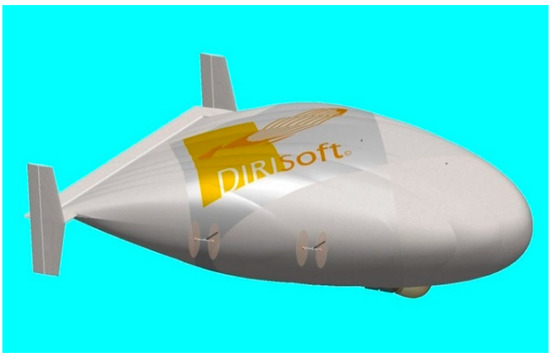
Figure 1.
The studied Airship.
In order to compensate for the airship’s great sensitivity to gusts of wind, it is over-actuated. Moreover, in order to make these aircraft accessible and interesting for different countries and parties, even those which lack infrastructure, it is necessary to consider handling at altitude. This requires the development of a precise autopilot to stabilise the airship around a point of loading or unloading. Various techniques have been proposed for the control and stabilisation of aerial vehicles, see for example Yang et al. [7] where a backstepping method was used, or Moutinho [8] where a path-tracking gain-scheduling controller is designed and its performance and robustness evaluated in a simulation environment. Note that the dynamic models of aerial vehicles are often assumed to be linear, obtained from the linearization of the nonlinear system around a specific operating point. In the same way, linear models are extensively studied in the literature. Even though they solve many problems, the applicability of such developed approaches may fail to stabilise the system or lead to degraded performances when the system operates far from the operating point where the linear model is valid. It is, therefore, interesting in certain cases to take into account the nonlinear behaviours in the system. This allows the enhancing of the control performances and enlarges the domain of applicability of the controllers.
Nonlinear behaviours are often present in practical systems, especially in flight systems, such as airships. Everyone agrees that the nonlinear systems are complex and difficult to study; they nonetheless allow the expression of the system behaviour with more accuracy and in a large domain of operation. Several classes of nonlinear systems are studied in the literature, such as Lipschitz systems, Linearizable systems by output injection, etc. Among the most interesting structures of nonlinear systems, we find the Quasi-Linear Parameter Varying (qLPV) models, as seen in Onat et al. [9]. An important advantage of these models is the possibility of scaling up tools designed for linear to non-linear systems. Many control and observation themes are, in fact, applied to this class of systems, in particular stability or stabilisation. Note that this class of systems can be represented in a polytopic form which converges to the form of the well-known Takagi–Sugeno Systems, as seen in Takagi et al. [10]. Stabilisation and control of nonlinear systems with qLPV representation is largely studied. We can cite the works of Tanaka et al. [11,12] and Guerra et al. [13], where a quadratic Lyapunov function was used to establish Linear Matrix Inequalities (LMIs) for controller design. For the sake of conservatism of the proposed solutions, relaxed stability conditions were obtained using, for example, the Tuan’s Lemma [14] or Polya’s theorem in Sala et al. [15]. This last study provides sufficient and asymptotic necessary conditions for stability and stabilisation by the use of quadratic Lyapunov functions seen in Hayat et al. [16]. Another way dealing with the conservatism reduction is the use of non-quadratic Lyapunov functions, as seen in Tanaka et al. [17], which produce more relaxed LMI conditions.
Concerning uncertain systems, the stabilisation problem still remains open in the case of uncertain Quasi-LPV model. For this class of systems, we find some works dealing only with the stabilisation problem and stability analysis, for example Cao et al. [18] and Ibrir et al. [19]. Hence, this paper presents a new approach based on the Quasi-LPV model representation with the aim of proposing a control for nonlinear dynamic systems with uncertainties. To the best of our knowledge, this method has never been tested for aerial vehicles. We have exploited the particularities of the airship in order to establish a stabilisation around an operating point within a polytope, which guarantees the stability of the flying object in a domain, and which takes into account possible uncertainties concerning the model or concerning the stresses which could impact the airship.
In this approach, designs based on the LMI method are used to find the feedback gains of a controller, as well as common P matrices (defined positive) satisfying a stability criterion derived in terms of the Lyapunov direct method.
2. Dynamics Model of the Airship
2.1. Kinematics
One can see in Figure 2 a reduced model of the airship. This last is assumed to be a rigid flying object. As usual in aeronautics, we use the parameterisation in yaw, pitch and roll (ψ, θ, φ) to define the orientation of the moving frame fixed to the centre of inertia G of the airship; with regard to the inertial frame and is a NED Cartesian frame, its origin being on the ground (Figure 2).
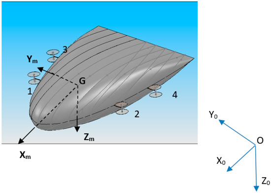
Figure 2.
The different reference frames.
The airship subject of our study is propelled by four rotors. Each rotor consists of two counter-rotating propellers. A given rotor i can rotate around two axes: the Ym-axis (βi), () and the ZRi-axis (γi) normal to Ym and which matches the Zm-axis (Figure 3) when βi = 0 (cruise flight); γi has these limitations: . A fictive axis XiR completes the rotor frame.
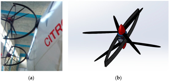
Figure 3.
(a) Thrusters of the airship; (b) CAD details of the thrusters.
Let be the thrust of rotor i; this force is positioned in the point Ti in Rm. The location of the different thrusters is established as follows:
The transformation matrix from Rm to R0 is defined by Goldstein [20]:
For simplicity, we will note by:
The speed of the airship in R0 is denoted by . It can be expressed with respect to the speed , which represents the speed expressed with respect to the local reference frame Rm, as is often the case in aeronautics.
Note that represents the position of the centre of inertia G. We also suppose that the distribution of masses is balanced between the top side and the bottom side of the airship, and thus the centre of volume coincides with the centre of gravity G.
Similarly, the speed of rotation with respect to the fixed reference frame could be expressed with respect to the angular speed of the airship in Rm as:
reciprocally:
The matrix J2 is defined as follows:
The overall kinematic relation of the airship can, therefore, be written in the following compact form:
2.2. Dynamical Model
The dynamic model of the flying body can be written in the following compact form, as seen in Shabana et al. [21]:
Here, is the vector of forces and torques applied on the airship. This includes the thrust of the rotors, the weight of the flying machine, the buoyancy Bu, as well as the lift and the aerodynamic drag.
Using the definitions of the thrusters, this vector will be written as:
and:
Remark 1.
In this study, we are only interested in the stabilisation of the airship around a fixed point of loading and unloading; the drag and lift forces will, therefore, not be taken into consideration. This is also the case for the effect of the elevator and rudders.
On the other hand, is the inertia matrix, according to the choice of the mobile reference frame, and is block-diagonal. The indices TT and RR correspond, respectively, to the inertias in translation and in rotation. This 6 × 6 matrix includes both the terms of inertia and the terms of added masses.
The latter reflect the increase in inertia of the solid under the effect of the resistance force of the fluid which surrounds the airship. This force depends on the acceleration of the moving solid body. Although these added masses can be neglected for airplanes or helicopters, this cannot be tolerated when the density of the solid body and that of the fluid which surrounds it are comparable, as in the case of airships or submarines, reported in Bennaceur et al. [6]. The calculation of these added masses can be performed experimentally or analytically as was done, for example, for the airship in Chaabani et al. [22].
Note that the over-actuation of the airship can generate certain complications in the calculation of the response of the actuators. The specific problem of control allocation was solved in a recent study by Azouz et al. [23]. In the aforementioned study, a control vector of dimension six was used as input, corresponding to the six degrees of freedom of the airship; the twelve degrees of freedom of the actuators (, βi and γi) were used as output. The system to be solved is rectangular. If this is done by means of numerical inversions, this can be penalizing for real-time control. The developed technique is based on energy concepts; this allows a quick and precise solution to the previous problem. This technique gave similar results to those obtained from other known techniques.
The components of the inertia matrix are denoted by Mij.
The gyroscopic forces and moments are grouped together within the vector: . is the cross product.
Taking into account Equations (8) and (9), the development of Equation (7) gives:
and:
This model will serve as a basis for the application of our control laws.
3. Quasi-LPV Representation for the Dynamic Model
3.1. Vector Control
To control the airship in hovering flight, the voltages at the terminals of the electric motors of the thrusters are varied, thus modifying the thrust forces Fi of the latter; the angles of inclination of the axes of these rotors are also varied by modifying the βi and γi. The airship, in this configuration, is fully actuated.
We must point out that we are interested in a case of stabilisation of the airship around a loading point. We assume that in this configuration the reference frames R0 and Rm are parallel and that the rotations of the airship are small.
The following control vector is proposed for the stabilisation of the airship:
and:
The dynamic model (10) and (11) becomes:
With:
In matrix form, the system (14) becomes:
with: being the vector of states, d = cos θ·cos φ is considered as a disturbance, and being the vector of control. Since we are stabilising the airship around a given point, and given the assumption made concerning the reference frames, we use the following kinematics relations: .
We should mention here that, for the specific problem at hand, the quadratic terms of type q·w are small and will be neglected later in the approach. The matrices A, B and E could be written as:
and:
One can choose the points of non-linearity as follows:
It is easy to check that all these points are bounded.
with:
Then, this matrix A becomes:
With z being the vector collection of the different zi.
The quasi-LPV method allows the expression of the behaviour of a system as a set of linear models. Each sub-model contributes to this total representation according to a weight function to value in the interval. The multi-model structure is written in the following form:
where . An example of a matrix Ai is detailed in Appendix A.1 in Appendix A.
The weighting functions hi are nonlinear, are given in Appendix A.1, and satisfy the following properties:
In summary, the proposed control strategy can be represented as follows (Figure 4):
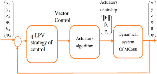
Figure 4.
Closed-loop architecture of control.
3.2. The Uncertain Matrix of the Airship
To test the reliability and the robustness of our method, we introduce uncertainty into many parameters of the airship. Mathematical models of Large Capacity Airships always contain uncertain elements, which model the designer’s lack of knowledge about certain parameter values, disturbances, and unmodelled dynamics. These uncertain parameters have values that are known only inside a given compact bounding set.
Let be the uncertain matrices having the same structure as .
We consider the following uncertain system:
where uncertainty is structured in the following way:
Such as are constant matrices defined later, and satisfy the following condition:
with I representing the identity matrix.
The uncertain matrix is given by:
One can see Appendix A.2 for more details regarding uncertain terms Δai.
With:
Using the expression (28), we can decompose the matrixes , and , in the following way:
Two further decompositions are as follows:
Other terms are all zero: and for , with:
To eliminate the term E·d of disturbance, we can suppose that:
Using the control expression (38), the Quasi-LPV structure of the airship is given by:
With:
where ;
We can choose the matrix S as: S =B+ E, where B+ is the pseudo-inverse matrix of the matrix B.
3.3. Robust Stabilisation of the Airship
Theorem 1.
The uncertain dynamic system (39) would be stable if there are definite, positive and symmetric matrixes P, and three positive diagonal matrixes and , such that the following LMIs and LME hold:
with: , and the matrix gains are defined by: , and
such as: for i = 1, …, 16.
To prove the above theorem, we must first recall the following lemmas which are useful in the proof:
Lemma 1.
Peterson [24]: Suppose F(t) satisfying, Q = QT, E, H are matrixes of appropriate dimension, the inequality below:
is regarded as met only when the following inequality is true for:
Lemma 2.
Let Ω be a positive definite matrix; for Y and X matrixes with compatible dimensions, the property below is true:
Lemma 3.
(Congruence) Consider two matrixes P and Q; if P is positive definite and if Q is a full column rank matrix, then the matrix is positive definite.
If P is a positive definite matrix, and if Q is a full column rank matrix, then the matrix product Q·P·QT is definite positive.
This lemma is called the congruence lemma
Lemma 4.
Boyd [25] (Schur Complement). Given constant matrixes with appropriate dimensions, where: and , then: if and only if:
Using these lemmas, the proof of Theorem 1 is presented as follows:
Proof.
Consider the Lyapunov function expressed as follows:
with being a definite positive matrix. □
The derivative with respect to time of V will then be:
And since we choose , the Equation (48) becomes:
As the weighting functions satisfy the property of convex sum, such that is negative, it is sufficient to check that:
We replace by its value (27), and we obtain:
Thereafter, and by relying on Lemma 1:
and as: and i = 1,2,3, then the inequality (51) becomes:
Based on Lemma 2, and if we suppose and , we obtain:
We can rewrite the system (52) as:
Finally, by using the Schur complement (Lemma 4), we will produce the following LMIs:
4. Simulation Results
We present here some numerical examples demonstrating the power of our formulation. As support for our development, we will use the following characteristics of the studied airship:
Mass: m = 500 Kg; gravity: g = 9.81 m·s−2;
Position of the centre of inertia zG = 0.5 m;
Buoyancy Bu = 5000 N;
Components of the total mass matrix M:
Uncertainty values:
The envelope:
Axis: a = 2.5 m; c = 2 m; Volume: V= 500 m3;
Position of the actuators: b1 = 5.4 m; b3 = 6.5 m;
The numerical developments were carried out using the MATLAB code.
As an illustration, we present a typical manoeuvre of a blimp over a loading area, which includes an attitude change due to a squall of wind. This change is estimated to rad in both pitch and roll motion.
Figure 5, Figure 6, Figure 7, Figure 8, Figure 9, Figure 10, Figure 11 and Figure 12 show the stabilisation of the angles of roll and pitch, as well as their derivatives, and the convergence of the linear velocities u, v and w, in a relatively short period of time.
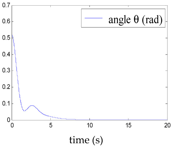
Figure 5.
Convergence of the pitch angle.
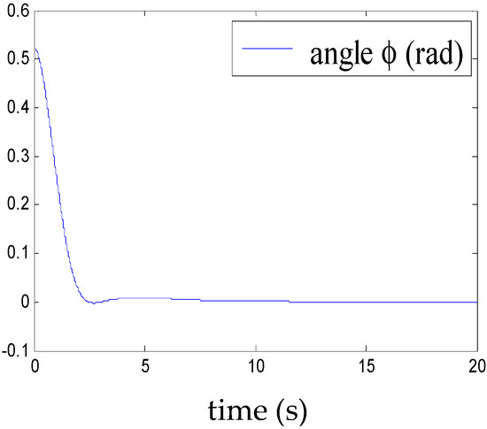
Figure 6.
Convergence of the roll angle.
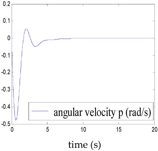
Figure 7.
Convergence of p.
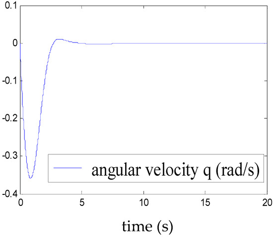
Figure 8.
Convergence of q.
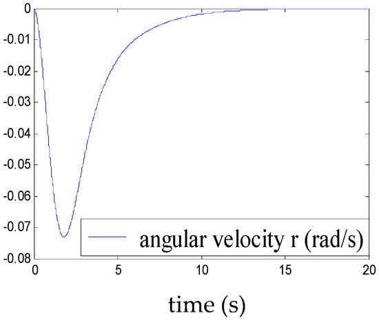
Figure 9.
Convergence of r.
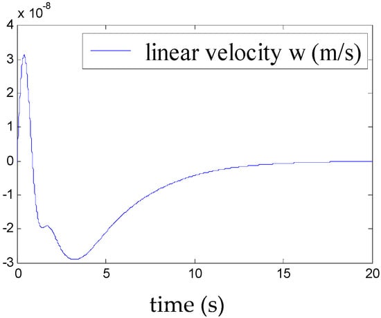
Figure 10.
Convergence of w.
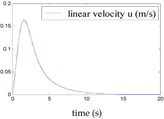
Figure 11.
Convergence of u.
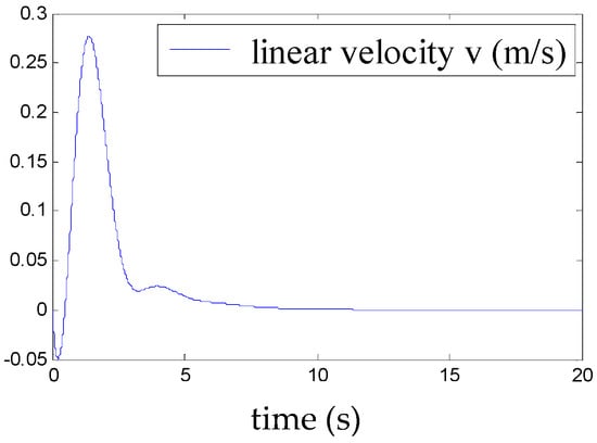
Figure 12.
Convergence of v.
This demonstrates the ability of the proposed control to stabilise the airship around a point of equilibrium, even under the effect of a moderate squall of wind. The time evolution of the weighting functions is depicted in Figure 13. It can be clearly seen that the weighting functions hi (1 ≤ i ≤ 8) are between 0 and 1 and thus satisfy the convex sum property.
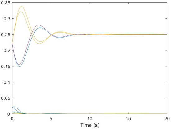
Figure 13.
The weighting function. The different colors represent the different weighting functions hi (1 ≤ i ≤ 8).
The robustness of the proposed control is also tested on the complete nonlinear model (28).
We note, according to Figure 14, Figure 15, Figure 16 and Figure 17, that even in the presence of a disturbance (presence of the wind) of maximum amplitude the 0.1, the airship remains stable. This demonstrates the performance of the elaborated control.
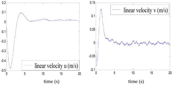
Figure 14.
Velocities u and v in presence of disturbance.
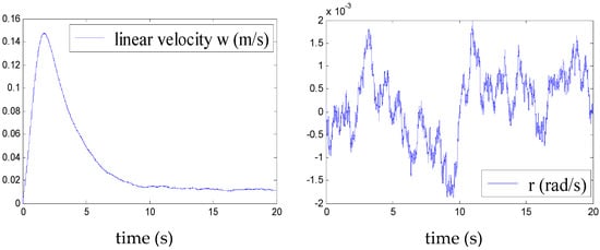
Figure 15.
Velocities w and r in presence of disturbance.
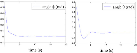
Figure 16.
Roll angle ϕ and pitch angle θ in the presence of disturbance.
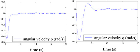
Figure 17.
Angular velocities p and q in the presence of disturbance.
5. Conclusions
In the first part of this paper, we presented a dynamic model of an unconventional airship. The latter has a flying wing shape and is over-actuated.
The stabilisation of this flying object at a point of equilibrium above a loading area was the highlight of this work.
Specifically, we have presented a controller design technique for uncertain nonlinear systems with external disturbances described by the Quasi-LPV model. The main results concern the two theorems developed to ensure a sufficient condition in terms of LMI for the problem of tracking uncertain systems, expressed in Quasi-LPV form. The results of the numerical simulations are satisfactory and prove the robustness of our approach.
Author Contributions
Conceptualization, S.C. and N.A.; Methodology, S.C. and N.A.; software, S.C.; validation, S.C. and N.A.; investigation, S.C. and N.A.; writing—original draft preparation, S.C. and N.A.; writing—review and editing, S.C. and N.A.; supervision, N.A.; project administration, S.C. and N.A. All authors have read and agreed to the published version of the manuscript.
Funding
This research received no external funding.
Institutional Review Board Statement
Not applicable.
Informed Consent Statement
Not applicable.
Data Availability Statement
The data presented in this study are available on request from the corresponding author.
Conflicts of Interest
The authors declare no conflict of interest.
Appendix A
Appendix A.1
The sub matrixes Ai were determined as follows:
The weighting functions were:
where: ; ; ; .
Appendix A.2
We determined the terms of uncertainties, as shown in the following example:
References
- Liao, L.; Pasternak, I. A review of airship structural research and developments. Prog. Aerosp. Sci. 2009, 45, 83–96. [Google Scholar] [CrossRef]
- Li, Y.; Nahon, M.; Sharf, I. Airship Dynamics modeling: A literature review. Prog. Aerosp. Sci. 2011, 47, 217–239. [Google Scholar] [CrossRef]
- Jex, H.; Gelhausen, P. Control response measurements of the Skyship 500 Airship. In Proceedings of the 6th AIAA Conference Lighter than Air Technology, Norfolk, VA, USA, 26 June–28 July 1985; pp. 130–141. [Google Scholar]
- Hygounenc, E.; Jung, I.K.; Soueres, P.; Lacroix, S. The autonomous blimp project of LAAS-CNRS: Achievements in flight control and terrain mapping. Int. J. Robot. Res. 2004, 23, 473–511. [Google Scholar] [CrossRef]
- El Omari, K.; Schall, E.; Koobus, B.; Dervieux, A. Inviscid flow calculation around flexible airship. In Proceedings of the Mathematical Symposium Garcia de Galdeano, Jaca, Spain, 15–17 September 2003; Volume 31, pp. 535–544. [Google Scholar]
- Bennaceur, S.; Azouz, N. Contribution of the added masses in the dynamic modelling of flexible airships. Nonlinear Dyn. 2012, 67, 215–226. [Google Scholar] [CrossRef]
- Yang, Y.; Wu, J.; Zheng, W. Positioning Control for an Autonomous Airship. J. Aircr. 2016, 53, 1638–1646. [Google Scholar] [CrossRef]
- Moutinho, A.; Azinheira, J.; Paiva, E.; Bueno, S.S. Airship robust path-tracking: A tutorial on airship modelling and gain-scheduling control design. Control Eng. Pract. 2016, 50, 22–36. [Google Scholar] [CrossRef]
- Onat, C.; Kucukdemiral, I.; Sivrioglu, S.; Yuksek, I. LPV Model Based Gain-scheduling Controller for a Full Vehicle Active Suspension System. J. Vib. Control 2007, 13, 1629. [Google Scholar] [CrossRef]
- Takagi, T.; Sugeno, M. Fuzzy identification of systems and its applications to modeling and control. IEEE Trans. Syst. Man Cybern. 1985, 15, 116–132. [Google Scholar] [CrossRef]
- Tanaka, K.; Ikeda, T.; Wang, H.O. Fuzzy regulators and fuzzy observers: Relaxed stability conditions and LMI-based designs. IEEE Trans. Fuzzy Syst. 1998, 6, 250–265. [Google Scholar] [CrossRef] [Green Version]
- Tanaka, K.; Wang, H.O. Fuzzy Control Systems Design and Analysis: A Linear Matrix Inequality Approach; John Wiley and Sons: Hoboken, NJ, USA, 2001. [Google Scholar]
- Guerra, T.M.; Kruszewski, A.; Vermeiren, L.; Tirmant, H. Conditions of output stabilization for nonlinear models in the Takagi-Sugeno’s form. Fuzzy Sets Syst. 2006, 157, 1248–1259. [Google Scholar] [CrossRef]
- Tuan, H.D.; Apkarian, P.; Narikiyo, T.; Yamamoto, Y. Parameterized linear matrix inequality techniques in fuzzy control system design. IEEE Trans. Fuzzy Syst. 2001, 9, 324–332. [Google Scholar] [CrossRef] [Green Version]
- Sala, A.; Arinõ, C. Asymptotically necessary and sufficient conditions for stability and performance in fuzzy control: Applications of Polya’s theorem. Fuzzy Sets Syst. 2007, 158, 2671–2686. [Google Scholar] [CrossRef]
- Hayat, A.; Shang, P. A quadratic Lyapunov function for Saint-Venant equations with arbitrary friction and space-varying slope. Automatica 2019, 100, 52–60. [Google Scholar]
- Tanaka, K.; Hori, T.; Wang, H.O. A multiple Lyapunov function approach to stabilization of fuzzy control systems. IEEE Trans. Fuzzy Syst. 2003, 11, 582–589. [Google Scholar] [CrossRef]
- Cao, Y.Y.; Frank, P.M. Analysis and synthesis of nonlinear time-delay systems via fuzzy control approach. IEEE Trans. Fuzzy Syst. 2000, 8, 200–211. [Google Scholar]
- Ibrir, S.; Botez, R. Robust stabilization of uncertain aircraft active systems. J. Vib. Control. 2005, 11, 187–200. [Google Scholar] [CrossRef]
- Goldstein, H. Classical Mechanics, 3rd ed.; Pearson, Ed.; Pearson: London, UK, 2001. [Google Scholar]
- Shabana, A. Dynamics of Multibody Systems, 5th ed.; Cambridge University Press: Cambridge, UK, 2020. [Google Scholar]
- Chaabani, S.; Azouz, N. Estimation of the Virtual Masses of a Large Unconventional Airship Based on Purely Analytical Method to Aid in the Preliminary Design. Aircr. Eng. Aerosp. Technol. 2021, 94, 531–540. [Google Scholar] [CrossRef]
- Azouz, N.; Khamlia, M.; Lerbet, J.; Abichou, A. Stabilization of an Unconventional Large Airship when Hovering. Appl. Sci. 2021, 11, 3551. [Google Scholar] [CrossRef]
- Petersen, I.R.; Hollot, C.V. A Riccati Equation Approach to the Stabilization of Uncertain Linear Systems. Automatica 1986, 22, 397–412. [Google Scholar] [CrossRef]
- Boyd, S.; Ghaoui, L.; Feron, E.; Balakrishnan, V. Linear Matrix Inequalities in Systems and Control Theory; SIAM: Philadelphia, PA, USA, 1994. [Google Scholar]
Publisher’s Note: MDPI stays neutral with regard to jurisdictional claims in published maps and institutional affiliations. |
© 2022 by the authors. Licensee MDPI, Basel, Switzerland. This article is an open access article distributed under the terms and conditions of the Creative Commons Attribution (CC BY) license (https://creativecommons.org/licenses/by/4.0/).