Three-Dimensional Impact Time Control Guidance Considering Field-of-View Constraint and Velocity Variation

Abstract

The problem of three-dimensional impact time control guidance considering field-of-view constraints and time-varying velocity is investigated in this study. First, considering the effect of gravity and aerodynamic forces on velocity, a simplified numerical estimation algorithm of flight time with a three-dimensional proportional navigation guidance law is derived. Then, based on the structure of the biased proportional navigation guidance law, the effect of the biased term on flight time is analyzed. The biased term is then designed to achieve impact time and field-of-view constraints considering time-varying velocity. Finally, numerical simulations are performed to demonstrate the effectiveness and superiority of the proposed guidance law.

1. Introduction

As a cost-effective and efficient combat method, the salvo attack has received extensive attention in recent years. There are two primary guidance methods to perform a salvo attack: impact time control guidance (ITCG) and cooperative guidance. With ITCG, multiple missiles should be assigned the same impact time. The missiles fly independently according to the specified ITCG law, and there is no communication between them. With cooperative guidance, there is communication between the missiles, which coordinate with each other to identify a common impact time. Both methods have certain advantages, and this paper primarily focuses on the ITCG method [1,2,3,4,5,6].

The design of the ITCG law should ensure the constraints of impact time and terminal miss distance. In addition, the field-of-view (FOV) constraint should also be considered. To adjust the flight time of the missile, the flight trajectory may become highly curved, which may lead to target locking failure of the seeker, causing the combat mission to fail. Many pieces of literature investigate the design of ITCG laws while considering the FOV constraint. In [7], a biased proportion navigation guidance (BPNG) law is designed. The biased term contains the impact time error, which is used to determine the impact time constraint. In addition, the cosine term of the lead angle is introduced to ensure the FOV constraint. In [8], a new switching surface that does not require time-to-go estimation is first designed. Then, a terminal sliding mode guidance law is designed to reach the switching surface. Finally, this ITCG law is modified to ensure the FOV constraint. In [9], the desired look angle that satisfies the impact angle and FOV constraints is determined. The desired look angle is a function of one adjustable gain, and the impact time constraint is achieved by adjusting the gain. Then, the ITCG law is derived to stabilize the real look angle to the desired look angle. In [10], the guidance process is divided into two phases. In phase 1, deviated pure pursuit (DPP) is used to keep the lead angle constant; in phase 2, the pure proportional navigation guidance (PPNG) law is used to ensure zero miss distance. The impact time is controlled by adjusting the switching point between the two phases. In addition, the lead angle does not increase in these two phases; thus, the FOV constraint is ensured. In [11], the guidance process is divided into two phases, and DPP is also used in phase 1. Different from [10], a new guidance law is used in phase 2 rather than the PPNG law. With the new guidance law, the lead angle constraint can be guaranteed, and the flight time can be solved analytically. In [12], a time-varying switching surface is first designed to ensure the impact time and FOV constraints. Then, a sliding mode guidance law is derived and modified to reach the switching surface.

These ITCG laws [7,8,9,10,11,12] can achieve the impact time and FOV constraints but have the same problem: they are derived based on the assumption of constant velocity. For missiles and guided projectiles flying in the atmosphere, thrust, aerodynamic forces and gravity can affect the velocity; thus, it is impractical to treat the velocity as constant in most cases. It is thus of practical importance to design ITCG laws that consider velocity variations, and some scholars have performed related research. In [13], an ITCG law that considers time-varying velocity is derived based on integral sliding mode control (ISMC). Using this method requires the expected range of missile velocities. In [14], the authors extend the existing time-to-go estimation algorithm under two-dimensional PPNG law to three-dimensional and design a new BPNG law, in which the biased term is used to eliminate the impact time error. Note that this method ignores the effect of gravity on velocity. In [15], a geometry-based impact time and angle control guidance (ITACG) law is designed for variable-speed unmanned aerial vehicles (UAVs). First, the flight trajectory is designed using Bezier curves, and then, the guidance command is obtained using inverse dynamics to track the designed trajectory. In [16], the effect of gravity on velocity is ignored, and the time-to-go estimation formula under the PNG law is derived. Then, the dynamics of the impact time error are analyzed, and the method in [1] is extended to consider velocity variations. In [17], assuming that the rate of change of velocity is a quadratic function of velocity, the time-to-go estimation formula under PNG law is derived, and then, the BPNG law is designed to achieve impact time control.

Although the methods in [13,14,15,16,17] consider velocity variations, none consider the effect of gravity on velocity. In [18], the ITCG law is derived based on the path-planning approach. The authors divide the flight trajectory into four segments, and this method can be extended to consider velocity variations using pre-flight analysis. However, this method does not consider the FOV constraint. In [19], the authors design the ITCG law through the look-angle shaping method. By predicting the future mean velocity, the method can also be extended to the case of velocity variation. However, this method is only applicable to two-dimensional engagement. In [20], the ITCG law is designed based on the data-driven method and PNG law. Using this method, a large offline database, which corresponds to a specific flight environment, must be established. When the real flight environment deviates from the flight environment of the database, the accuracy of the offline database will likely decrease. Therefore, the adaptability of this method to the flight environment is insufficient. In [21,22], the authors first derive the numerical estimation algorithm of time-to-go under the PNG law and then design a biased term for the PNG law to control the impact time. Note that the biased terms in [21,22] are given directly based on the feedback of impact time error, and there is no theoretical analysis or proof process. The biased term actually affects the length of the flight trajectory and the induced drag force, both of which can affect the impact time. In addition, the estimation algorithm in [21] uses a recursive algorithm, which may lead to a high computational burden on the onboard computer, while the estimation algorithm in [22] is only applicable to two-dimensional engagement.

Based on this review, the problem of three-dimensional impact time control guidance that considers field-of-view constraints and time-varying velocity is addressed in this study. Considering the unpowered flight of a guided projectile in the terminal guidance phase, a novel numerical estimation algorithm of time-to-go under the three-dimensional PNG law is derived. The effect of the aerodynamic forces and gravity on projectile velocity is fully considered in this algorithm. Then, the biased term is designed based on the PNG law. The effect of the biased term on flight time is analyzed, and the analysis results are given in the form of a theorem. Finally, numerical simulations are performed to verify the effectiveness of the proposed time-to-go estimation algorithm and ITCG law.

The primary advantages of the method proposed in this paper can be summarized as follows. First, compared with [7,8,9,10,11,12], the proposed method satisfies the impact time and FOV constraints and can consider velocity variations. Second, compared with [13,14,15,16,17], the proposed method fully considers the effect of aerodynamic forces and gravity on velocity. Third, the proposed method analyzes the effect of the biased term on flight time and yields a sufficient condition for the design of the biased term, while the theoretical analysis is not performed in [21,22]. In addition, the method in [22] is only applicable to two-dimensional engagement while the proposed method can be applied to three-dimensional engagement.

The remainder of this paper is organized as follows. In Section 2, the guidance and dynamic models of the guided projectile are introduced, and the impact time control problem is described. In Section 3, a simplified numerical estimation algorithm of time-to-go under the three-dimensional PNG law is given. In Section 4, the effect of the biased term on flight time is analyzed, and the ITCG law considering FOV constraint and velocity variation is designed. Numerical simulation and comparisons are performed in Section 5, and the conclusions are given in Section 6.

2. Problem Statement and Guidance Model Analysis

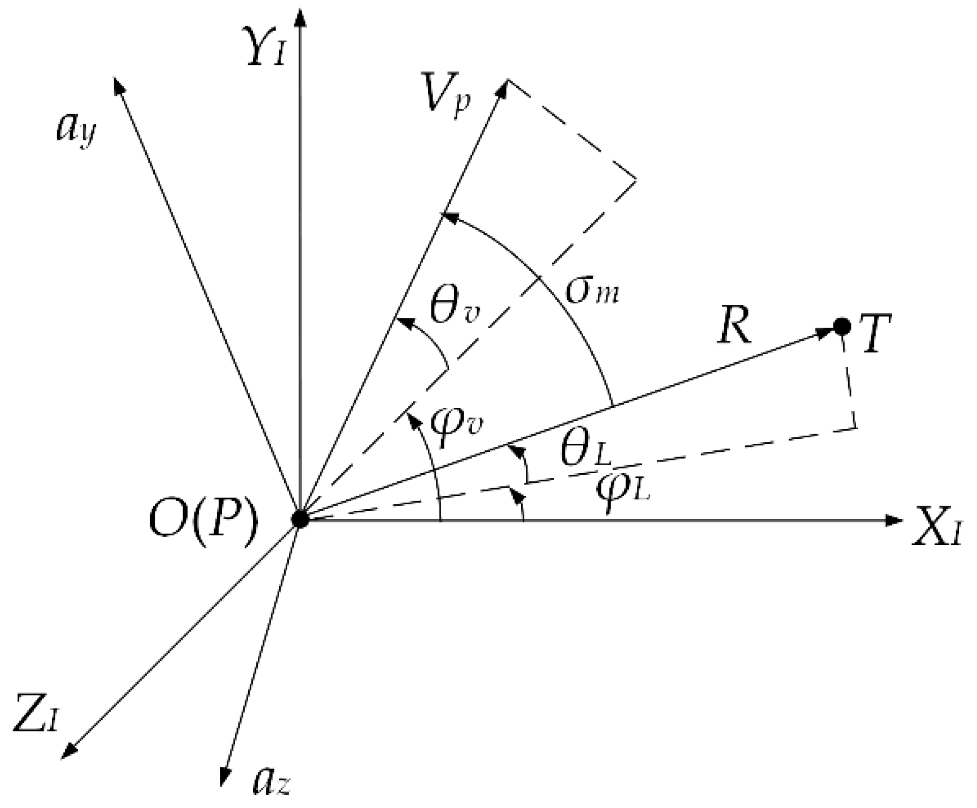
2.1. Problem Statement

The three-dimensional homing engagement geometry between a guided projectile P and a stationary target T is shown in Figure 1, where OX_IY_IZ_I is the inertial reference coordinate system. The coordinates of the guided projectile and target are denoted as (x_p, y_p, z_p) and (x_T, y_T, z_T), respectively. The projectile velocity is denoted as V_p, and the relative distance between the projectile and target is denoted as R. The angles φ_L and θ_L denote the line-of-sight (LOS) angle in the azimuth and elevation directions, respectively. θ_v is the flight path angle, and φ_v is the heading angle. The velocity lead angle is denoted as σ_m. a_y is the normal acceleration of the projectile defined in the longitudinal plane, and a_z is the lateral acceleration defined in the lateral plane. Both a_y and a_z are perpendicular to the velocity and should be designed.

The nonlinear engagement equations between the guided projectile and stationary target in three-dimensional space can be written as [23]:

$$\begin{array}{l}\dot{R}=-V_p\sin {\theta }_L\sin {\theta }_v-V_p\cos {\theta }_L\cos {\theta }_v\cos ({\phi }_L-{\phi }_v)\\ {\dot{\theta }}_L=\frac{V_p}{R}\left[\sin {\theta }_L\cos {\theta }_v\cos ({\phi }_L-{\phi }_v)-\cos {\theta }_L\sin {\theta }_v\right]\\ {\dot{\phi }}_L=\frac{V_p}{R\cos {\theta }_L}\cos {\theta }_v\sin ({\phi }_L-{\phi }_v)\\ {\dot{\theta }}_v=\frac{a_y-g\cos {\theta }_v}{V_p}\\ {\dot{\phi }}_v=-\frac{a_z}{V_p\cos {\theta }_v}\end{array}$$

(1)

The relationship between the coordinates of the guided projectile and target can also be described by:

$$\begin{array}{l}{x}_p=x_T-R\cos {\theta }_L\cos {\phi }_L\\ y_p=y_T-R\sin {\theta }_L\\ z_p=z_T+R\cos {\theta }_L\sin {\phi }_L\end{array}$$

(2)

The terminal guidance phase of the guided projectile is unpowered; thus, aerodynamic forces and gravity have a great influence on velocity. Therefore, the dynamics of the guided projectile must be considered, and the three-degree-of-freedom dynamic equations are as follows [24]:

$$\begin{array}{l}{\dot{V}}_p=\frac{1}{m}(-F_D-mg\sin {\theta }_v)\\ {\dot{\theta }}_v=\frac{1}{m{V}_p}(F_L-mg\cos {\theta }_v)\\ {\dot{\phi }}_v=-\frac{1}{m{V}_p\cos {\theta }_v}{F}_C\end{array}$$

(3)

where m is the projectile mass and g is the gravitational acceleration; and F_D, F_L, and F_C are the drag, lift, and side force, respectively. For guided projectiles flying in the atmosphere, the total angle of attack is usually small and the aerodynamic forces can be written as:

$$\begin{array}{l}{F}_D=\frac{1}{2}\rho V_p^{2}S{C}_{D0}\left[1+k_b({\alpha }^2+{\beta }^2)\right]\\ F_L=\frac{1}{2}\rho V_p^{2}S{C}_{L\alpha }\alpha \\ F_C=\frac{1}{2}\rho V_p^{2}S{C}_{C\beta }\beta \end{array}$$

(4)

where ρ is the air density, S is the reference area, α is the angle of attack and β is the sideslip angle. C_D0 is the zero-lift drag coefficient, k_b is the induced drag force coefficient, C_Lα is the derivative of the lift force coefficient, and C_Cβ is the derivative of the side force coefficient. Each of these aerodynamic coefficients can be obtained from a table generated from the wind tunnel experiments.

The real flight time of the guided projectile is denoted as T_f, and the designated flight time is denoted as T_d. The time-to-go at moment t is denoted as t_go, and the impact time error is denoted as e, which can be expressed as follows:

$$e=T_d-t-t_{go}$$

(5)

To achieve impact time control of the guided projectile, the flight time T_f should be equal to the specified time T_d. To adjust the impact time, the flight trajectory may become highly curved. Considering the limited detection capability of the seeker, the seeker may not be able to guarantee target lock, which may lead to the failure of the combat mission. The lock-on condition of the seeker can be approximately represented by the lead angle constraint. In addition, considering the limited control ability of the guided projectile, the acceleration command cannot exceed the maximum acceleration that the projectile can provide. The above constraints can be mathematically described as:

$$\begin{array}{l}R(T_f)=0\\ T_f=T_d\\ 0\le {\sigma }_m\le {\sigma }_{\max }\\ \left|a_y\right|\le a_{\max },\left|a_z\right|\le a_{\max }\end{array}$$

(6)

where σ_max is the upper bound of σ_m, and a_max is the maximum acceleration command that the guided projectile can provide.

Therefore, the design goal of this paper can be described as designing the normal acceleration command a_y and lateral acceleration command a_z so that the guided projectile can meet constraint (6).

2.2. Guidance Model Analysis

It is convenient to consider projectile dynamics (3) based on (1). However, when considering the FOV constraint, it is inconvenient to use (1), which is not conducive to the subsequent model simplification. Based on these considerations, another guidance model described by (R, θ_L, φ_L, θ_m, φ_m) rather than (R, θ_L, φ_L, θ_v, φ_v) is given as follows [25]:

$$\begin{array}{l}\dot{R}=-V_p\cos {\theta }_m\cos {\phi }_m=-V_p\cos {\sigma }_m\\ {\dot{\theta }}_L=-\frac{V_p}{R}\sin {\theta }_m\\ {\dot{\phi }}_L=-\frac{V_p}{R\cos {\theta }_L}\cos {\theta }_m\sin {\phi }_m\\ {\dot{\theta }}_m=\frac{a_{ym}}{V_p}+\frac{V_p}{R}\tan {\theta }_L\cos {\theta }_m{\sin }^2{\phi }_m+\frac{V_p}{R}\sin {\theta }_m\cos {\phi }_m\\ {\dot{\phi }}_m=-\frac{a_{zm}}{V_p\cos {\theta }_m}-\frac{V_p}{R}\tan {\theta }_L\sin {\theta }_m\sin {\phi }_m\cos {\phi }_m+\frac{V_p}{R\cos {\theta }_m}\sin {\phi }_m\end{array}$$

(7)

where θ_m and φ_m are the velocity lead angle defined in the LOS frame; and a_ym and a_zm are the acceleration components in the pitch and yaw directions, respectively. Both a_ym and a_zm are perpendicular to the velocity. Note that the guidance models in (1) and (7) are not independent, and there is a conversion relationship between (θ_m, φ_m) and (θ_v, φ_v) as follows:

$$\begin{array}{l}\sin {\theta }_m=\cos {\theta }_L\sin {\theta }_v-\sin {\theta }_L\cos {\theta }_v\cos ({\phi }_L-{\phi }_v)\\ \sin {\phi }_m=-\frac{\cos {\theta }_v}{\cos {\theta }_m}\sin ({\phi }_L-{\phi }_v)\end{array}$$

(8)

The two coordinate systems used to define (a_ym, a_zm) in (7) and (a_y, a_z) in (1) are different. Thus, a_ym and a_zm are not equal to a_y and a_z. The relationship between them can be described by:

$$\begin{array}{l}{a}_y=a_{ym}\cos \gamma +a_{zm}\sin \gamma +g\cos {\theta }_v\\ a_z=-a_{ym}\sin \gamma +a_{zm}\cos \gamma \end{array}$$

(9)

where γ is a rotation angle and can be described by:

$$\sin \gamma =\sin {\theta }_L\frac{\sin ({\phi }_v-{\phi }_L)}{\cos {\theta }_m}$$

(10)

Based on (7), the three-dimensional PNG law is given as follows [25]:

$$\begin{array}{l}{a}_{ym}=a_{ymP}=-\frac{N{V}_p^2}{R}\sin {\theta }_m\cos {\phi }_m\\ a_{zm}=a_{zmP}=\frac{N{V}_p^2}{R}\sin {\phi }_m\end{array}$$

(11)

where N is the navigation gain. In the following sections, an ITCG law considering the FOV constraint and velocity variation is designed based on PNG law (11).

Remark 1.

Guidance models (1) and (7) have their own advantages in dynamic analysis and FOV constraint analysis, respectively. In the following contents, the guidance model (7) is simplified to design a three-dimensional time-to-go estimation algorithm, and a BPNG law is designed based on PNG law (11) and conversion relationship (9). In the numerical simulations, guidance model (1) is used because it is more convenient to simulate the projectile dynamics. In addition, the acceleration command of the guided projectile is usually given in the form of a_y and a_z rather than a_ym and a_zm.

3. Three-Dimensional Time-to-Go Estimation under Time-Varying Velocity

In this section, a novel time-to-go estimation algorithm that considers time-varying velocities under PNG law (11) is presented. Considering the real dynamics of the guided projectile, the flight time under PNG law (11) cannot be solved analytically; thus, a numerical solution is required. Limited by the computing power of the onboard computer, it is not advisable to solve the complete guidance and dynamic equations. Therefore, it is necessary to design a faster and high-precision time-to-go estimation algorithm for guided projectiles.

In practical applications, the terminal guidance phase generally follows a precise guidance handover from midcourse guidance; thus, the initial value of the lead angle σ_m is usually small [26]. Therefore, we can make the following approximation:

$$\begin{array}{l}\sin {\sigma }_m\approx {\sigma }_m,\cos {\sigma }_m\approx 1\\ \sin {\theta }_m\approx {\theta }_m,\cos {\theta }_m\approx 1\\ \sin {\phi }_m\approx {\phi }_m,\cos {\phi }_m\approx 1\end{array}$$

(12)

and (7) can be simplified to:

$$\begin{array}{l}\dot{R}=-V_p\\ {\dot{\theta }}_L=-\frac{V_p}{R}{\theta }_m\\ {\dot{\phi }}_L=-\frac{V_p}{R\cos {\theta }_L}{\phi }_m\\ {\dot{\theta }}_m=\frac{a_{ym}}{V_p}+\frac{V_p}{R}{\theta }_m\\ {\dot{\phi }}_m=-\frac{a_{zm}}{V_p}+\frac{V_p}{R}{\phi }_m\end{array}$$

(13)

The PNG law (11) can also be simplified to:

$$\begin{array}{l}{a}_{ym}=a_{ymP}=-\frac{N{V}_p^2}{R}{\theta }_m\\ a_{zm}=a_{zmP}=\frac{N{V}_p^2}{R}{\phi }_m\end{array}$$

(14)

Substituting (14) into (13), we can obtain:

$$\begin{array}{l}\frac{d{\theta }_m}{dR}=\frac{(N-1)}{R}{\theta }_m\\ \frac{d{\phi }_m}{dR}=\frac{(N-1)}{R}{\phi }_m\end{array}$$

(15)

By integrating (15), the functions of θ_m and φ_m concerning R can be described as follows:

$$\begin{array}{l}{\theta }_m={\theta }_{m0}{(\frac{R}{R_0})}^{N-1}\\ {\phi }_m={\phi }_{m0}{(\frac{R}{R_0})}^{N-1}\end{array}$$

(16)

where θ_m0, φ_m0, and R₀ are the initial values of θ_m, φ_m, and R, respectively. The velocity lead angle σ_m can also be obtained according to (7) and (16) as:

$${\sigma }_m=\arccos (\cos {\theta }_m\cos {\phi }_m)$$

(17)

Substituting (16) into (13), the function of θ_L concerning R can be described by:

$${\theta }_L={\theta }_{L0}+\frac{{\theta }_{m0}}{(N-1)}\left[{\left(\frac{R}{R_0}\right)}^{N-1}-1\right]$$

(18)

where θ_L0 is the initial value of θ_L.

According to (10) and (12), we obtain γ as a small angle; thus, (9) can be approximated as follows:

$$\begin{array}{l}{a}_y\approx a_{ym}+g\cos {\theta }_v\\ a_z\approx a_{zm}\end{array}$$

(19)

Thus, we can obtain:

$$\begin{array}{l}{a}_y=V_p{\dot{\theta }}_v+g\cos {\theta }_v\approx a_{ym}+g\cos {\theta }_v=-\frac{N{V}_p^2{\theta }_m}{R}+g\cos {\theta }_v=N{V}_p{\dot{\theta }}_L+g\cos {\theta }_v\\ a_z=-V_p\cos {\theta }_v{\dot{\phi }}_v\approx a_{zm}=\frac{N{V}_p^2{\phi }_m}{R}=-N{V}_p\cos {\theta }_L{\dot{\phi }}_L\approx -N{V}_p\cos {\theta }_v{\dot{\phi }}_L\end{array}$$

(20)

According to (20), the PNG law (11) can be approximated to the traditional PPNG law under the small lead angle assumption, and we can obtain:

$$\begin{array}{l}{\dot{\theta }}_v=N{\dot{\theta }}_L\\ {\dot{\phi }}_v=N{\dot{\phi }}_L\end{array}$$

(21)

By integrating (21) and combining (18), we can obtain:

$${\theta }_v={\theta }_{v0}+\frac{N{\theta }_{m0}}{(N-1)}\left[{\left(\frac{R}{R_0}\right)}^{N-1}-1\right]$$

(22)

where θ_v0 is the initial value of θ_v. The air density ρ can be expressed as a function of altitude y_p as follows [27]:

$$\rho =\{\begin{array}{l}1.232e^{-0.1024\times y_p/1000},y_p\le 6000\\ 1.374e^{-0.1207\times y_p/1000},6000<y_p\le \mathrm{11,000}\\ 2.059e^{-0.1572\times y_p/1000},y_p>\mathrm{11,000}\end{array}$$

(23)

Note that the flight altitude y_p of the guided projectile can be obtained from (2) and (18) as:

$$y_p=y_T-R\sin \left\{{\theta }_{L0}+\frac{{\theta }_{m0}}{(N-1)}\left[{\left(\frac{R}{R_0}\right)}^{N-1}-1\right]\right\}$$

(24)

Thus, the air density ρ can also be expressed as a function of R.

In this analysis, we can obtain the functions of θ_m, φ_m, σ_m, θ_L, θ_v, y_p, and ρ concerning R under guidance law (11). According to (3) and (7), the final differential equations used for t_go estimation are as follows:

$$\frac{dt}{dR}=-\frac{1}{V_p\cos {\sigma }_m}$$

(25)

$$\begin{array}{ll}\frac{d{V}_p}{dR}& =\frac{1}{m{V}_p\cos {\sigma }_m}(F_D+mg\sin {\theta }_v)\\ & =\frac{g\sin {\theta }_v}{V_p\cos {\sigma }_m}+\frac{qS{C}_{D0}}{m{V}_p\cos {\sigma }_m}\left[1+k_b({\alpha }^2+{\beta }^2)\right]\\ & =\frac{qS{C}_{D0}+mg\sin {\theta }_v}{m{V}_p\cos {\sigma }_m}+\frac{m{k}_b{C}_{D0}}{qS{V}_p\cos {\sigma }_m}\left[{\left(\frac{a_y}{C_{L\alpha }}\right)}^2+{\left(\frac{a_z}{C_{c\beta }}\right)}^2\right]\\ & \approx \frac{qS{C}_{D0}+mg\sin {\theta }_v}{m{V}_p\cos {\sigma }_m}+\frac{m{k}_b{C}_{D0}}{qS{V}_p\cos {\sigma }_m}\left[{\left(\frac{a_{ymp}+g\cos {\theta }_v}{C_{L\alpha }}\right)}^2+{\left(\frac{a_{zmp}}{C_{c\beta }}\right)}^2\right]\end{array}$$

(26)

Using (25) and (26), we can obtain the estimated flight time T_e under PNG law (11). In addition, we can also obtain the estimated time-to-go t_goe and the estimation error e_c at moment t.

Remark 2.

The numerical solution of differential Equations (25) and (26) requires the aerodynamic coefficients C_D0, C_Lα, C_cβ, k_b, and gravitational acceleration g. For the terminal guidance process of the guided projectile, the flight time is typically short; thus, the changes in velocity and gravitational acceleration are small. Therefore, the aerodynamic coefficients and gravitational acceleration are treated as constants in this paper. It is also feasible to consider the effect of changes in these parameters on the t_go estimation. We thus update the parameter values based on the current V_p and R of each step in the integration.

Remark 3.

The proposed estimation algorithm has two advantages in numerical calculation: (1) the number of differential equations to be solved is reduced, and only two differential equations must be solved; and (2) the relative distance R is used as the integration variable. To increase computational efficiency and estimation accuracy, the integration step size can be selected as a large value, which will be verified in the next numerical simulation. Therefore, the computational burden can be markedly reduced.

4. Three-Dimensional ITCG Law Design

4.1. Analysis of the Biased Term

In this study, the ITCG law is designed based on PNG law (11) and the conversion relationship (9). To reduce the complexity of the design, only the pitch direction is added with the biased term, and the PNG law a_zmp is used in the yaw direction. Therefore, the guidance command represented by a_ym and a_zm is designed as follows:

$$\begin{array}{l}{a}_{ym}=a_{ymp}+\Delta a_{ym}=-\frac{N}{R}{V}_p^2\sin {\theta }_m\cos {\phi }_m+\Delta a_{ym}\\ a_{zm}=a_{zmp}=\frac{N}{R}{V}_p^2\sin {\phi }_m\end{array}$$

(27)

where Δa_ym is the biased term that should be designed. The final acceleration command (a_y, a_z) can be obtained through the conversion relationship (9) and can be approximately expressed as (19) when the lead angle is small.

In most studies of ITCG law design that considers velocity variations, the effects of gravity are typically ignored. However, this omission is not suitable for the terminal guidance phase of the guided projectile. Few studies [21,22] consider the effects of gravity and design ITCG laws based on the BPNG structure. Note that the biased term affects the length of the flight trajectory and the drag force, both of which can affect the impact time. Therefore, when considering the velocity variation, the influence of the biased term on flight time is complex. Unfortunately, [21,22] do not provide a theoretical analysis; thus, the scope of application of these methods is unclear. Therefore, we first analyze the influence of the biased term on flight time and then design the biased term.

Different from starting with the analytical formula of t_go, this paper adjusts the acceleration component along the LOS through Δa_ym to adjust the time for R to converge to 0. For simplicity, we define the function f_d concerning Δa_ym as follows:

$$f_d=\frac{m{k}_b{C}_{D0}\cos {\sigma }_m}{qS{C}_{L\alpha }^2}\Delta a_{ym}\left[\Delta a_{ym}+2(a_{ymp}+g\cos {\theta }_v)+\frac{qS{C}_{L\alpha }^2}{m{k}_b{C}_{D0}}\tan {\theta }_m\right]$$

(28)

The analysis results are described in Theorem 1.

Theorem 1.

For a guided projectile flying at a small lead angle under guidance law (27), the biased term Δa_ym can adjust the flight time, and the results are as follows:

(1) 

If f_d > 0, the biased term Δa_ym can increase the flight time of the projectile;

(2) 

If f_d = 0, the biased term Δa_ym does not affect the flight time of the projectile;

(3) 

If f_d < 0, the biased term Δa_ym can decrease the flight time of the projectile.

Proof of Theorem 1.

According to (7), the second derivative of R with respect to t can be described by:

$$\begin{array}{ll}\ddot{R}& =\frac{\cos {\sigma }_m}{m}(F_D+mg\sin {\theta }_v)+V_p\sin {\theta }_m\cos {\phi }_m{\dot{\theta }}_m+V_p\cos {\theta }_m\sin {\phi }_m{\dot{\phi }}_m\\ & =\frac{\cos {\sigma }_m}{m}{F}_D+\sin {\theta }_m\cos {\phi }_m{a}_{ym}-\sin {\phi }_m{a}_{zm}+g\sin {\theta }_v\cos {\sigma }_m+\frac{V_p^2}{R}{\sin }^2{\sigma }_m\\ & \approx \frac{\cos {\sigma }_m}{m}qS{C}_{D0}\left[1+k_b{(\frac{m\Delta a_{ym}}{qS{C}_{L\alpha }}+{\alpha }_p)}^2+k_b{\beta }_p^2\right]+\sin {\theta }_m\cos {\phi }_m(a_{ymp}+\Delta a_{ym})\\ & -\sin {\phi }_m{a}_{zmp}+g\sin {\theta }_v\cos {\sigma }_m+\frac{V_p^2}{R}{\sin }^2{\sigma }_m\\ & =\frac{\cos {\sigma }_m}{m}qS{C}_{D0}{k}_b(\frac{m^2\Delta a_{ym}^2}{q^2{S}^2{C}_{L\alpha }^2}+\frac{2m{\alpha }_p\Delta a_{ym}}{qS{C}_{L\alpha }})+\sin {\theta }_m\cos {\phi }_m\Delta a_{ym}+C_1\\ & =f_d+C_1\end{array}$$

(29)

where:

$$\begin{array}{l}{\alpha }_p=\frac{m(a_{ymp}+g\cos {\theta }_v)}{qS{C}_{L\alpha }}\\ {\beta }_p=\frac{m{a}_{zmp}}{qS{C}_{c\beta }}\\ C_1=\frac{\cos {\sigma }_m}{m}qS{C}_{D0}(1+k_b{\alpha }_p^2+k_b{\beta }_p^2)+\sin {\theta }_m\cos {\phi }_m{a}_{ymp}\\ -\sin {\phi }_m{a}_{zmp}+g\sin {\theta }_v\cos {\sigma }_m+\frac{V_p^2}{R}{\sin }^2{\sigma }_m\end{array}$$

(30)

In (29), C₁ represents the acceleration component along the LOS under PNG law (11), while the effect of the biased term Δa_ym is concentrated on f_d. For small lead angle flight, we can obtain $\dot{R}<0$ according to (7). If $f_d>0$, $\ddot{R}$ increases compared with that under the PNG law, and the next $\dot{R}$ will also increase. Therefore, the relative distance R decreases more slowly, and the flight time is increased compared with under the PNG law. Similarly, if $f_d<0$, $\ddot{R}$ decreases compared with that under the PNG law, and the next $\dot{R}$ will also decrease. Therefore, the relative distance R decreases faster, and the flight time decreases compared with under the PNG law. If $f_d=0$, the biased term does not affect the flight time. This completes the proof.

Theorem 1 yields a sufficient condition for adjusting the flight time of the guided projectile, which can be used as a basis for designing the biased term. In addition, based on Theorem 1, we give two corollaries to simplify the design of the biased term in specific cases. For simplicity, we define R_c as follows:

$$R_c=\frac{4mN{k}_b{C}_{D0}\cos {\sigma }_m}{\rho S{C}_{L\alpha }^2}$$

(31)

and the corollaries are given as follows. □

Corollary 1.

For a guided projectile flying at a small lead angle under guidance law (27), if ${\theta }_m\ge 0$ and $R\ge R_c$, the flight time can be increased if ${\Delta a}_{ym}>0$.

Proof of Corollary 1.

For $R\ge R_c$, it can be determined that:

$$R\ge R_c=\frac{4mN{k}_b{C}_{D0}\cos {\sigma }_m}{\rho S{C}_{L\alpha }^2}\frac{0.5V_p^2}{0.5V_p^2}=\frac{2N{V}_p^2\cos {\sigma }_{m}m{k}_b{C}_{D0}}{qS{C}_{L\alpha }^2}$$

(32)

Rearranging (32) and considering that ${\theta }_m\ge 0$, we can obtain:

$$\frac{2N{V}_p^2\cos {\phi }_m\sin {\theta }_m}{R}\le \frac{qS{C}_{L\alpha }^2\sin {\theta }_m}{m{k}_b{C}_{D0}\cos {\theta }_m}$$

(33)

Note that $f_d=0$ has two zero points, and the nonzero zero point is denoted as C₂. Then, (28) can be rewritten as:

$$f_d=C_3\Delta a_{ym}(\Delta a_{ym}-C_2)$$

(34)

where:

$$\begin{array}{ll}{C}_2& =-2a_{ymp}-2g\cos {\theta }_v-\frac{qS{C}_{L\alpha }^2}{m{k}_b{C}_{D0}}\tan {\theta }_m\\ & =\frac{2N{V}_p^2\cos {\phi }_m\sin {\theta }_m}{R}-\frac{qS{C}_{L\alpha }^2}{m{k}_b{C}_{D0}}\tan {\theta }_m-2g\cos {\theta }_v\\ & <0\end{array}$$

(35)

$$C_3=\frac{m{k}_b{C}_{D0}\cos {\sigma }_m}{qS{C}_{L\alpha }^2}>0$$

(36)

Therefore, for ${\theta }_m\ge 0$ and $R\ge R_c$, if ${\Delta a}_{ym}>0$, we can obtain f_d > 0, and the flight time can be increased according to Theorem 1. This completes the proof. □

Corollary 2.

For a guided projectile flying at a small lead angle under guidance law (27), if ${\theta }_m\le 0$ and $R\le R_c$, the flight time can be increased if ${\Delta a}_{ym}>0$.

The proof process of Corollary 2 is similar to that of Corollary 1; thus, the proof is not given in this study.

Remark 4.

In (27), the biased term is added only in the pitch plane, and the PNG law is used in the yaw plane. The purpose of this design is to simplify the design process and facilitate the analysis of the effect of the biased term on the flight time. Obviously, the analysis with two biased terms is more complicated than just one biased term. Subsequent research can consider adding biased terms in both planes to obtain the ITCG law with optimal control energy. In addition, the flight process of guided projectile under ITCG law (27) can be divided into two phases. Phase 1 is used to adjust the flight time, and phase 2 is used to ensure the terminal interception. In phase 1, the biased term works to adjust the flight time of guided projectile, and both impact time error and the biased term converge to 0; in phase 2, the biased term is 0, and both planes are governed by the PNG law to ensure terminal interception. Even if the impact time error cannot converge to 0 in phase 1, the flight process will still convert to phase 2 because the terminal interception is more important than adjusting the flight time.

Remark 5.

Theorem 1 and Corollaries 1 and 2 are sufficient conditions for adjusting the flight time of the guided projectile. Failure to meet these three conditions does not mean that the flight time cannot be adjusted. Corollaries 1 and 2 are special cases of Theorem 1, and the biased term designed based on Corollaries 1 and 2 is more conservative. In addition, the flight time in the terminal guidance phase is relatively short; thus, the change in R_c is small and can be approximated to be a constant, which is convenient when using Corollaries 1 and 2 to design the biased term. Note that the choice of N has an effect on R_c. The larger the N, the larger the R_c, and the faster the impact time error needs to converge. Therefore, a larger biased term needs to be designed, and a larger acceleration command needs to be provided by the projectile. The advantage of a larger R_c is that it ensures faster convergence of impact time error, and thus the ITCG law can be converted to the PNG law faster to ensure the terminal interception. Therefore, the value of N needs to be selected according to the actual combat requirements and the performance of the guided projectile. In this paper, N = 3 is taken as an example for simulation analysis.

4.2. ITCG Law Design

For the problem of impact time control guidance, due to the small lead angle flight in the terminal guidance phase, the flight time that the projectile can reduce is limited. Therefore, this study considers the issue of increasing the flight time. When the velocity direction is above the LOS in the terminal guidance phase (i.e., ${\theta }_m\ge 0$), the biased term designed based on Corollary 1 is as follows:

$$\Delta a_{ym}=k_1{\left|e\right|}^{\alpha }\mathrm{sgn}(e)\epsilon (R)\delta (\frac{{\sigma }_m}{{\sigma }_{\max }})$$

(37)

where:

$$\epsilon (x)=\{\begin{array}{l}1,x\ge R_{ce}\\ 0,x\le (1-k_2)R_{ce}\\ -\frac{2}{{(k_2{R}_{ce})}^3}{x}^3+\frac{3(2-k_2)R_{ce}}{{(k_2{R}_{ce})}^3}{x}^2-\frac{6(1-k_2)R_{ce}^2}{{(k_2{R}_{ce})}^3}x+\frac{k_2^3-3k_2+2}{k_2^3},else\end{array}$$

(38)

$$\delta (x)=\frac{e^{k_3}-e^{k_{3}x}}{e^{k_3}-1}$$

(39)

In (38), R_ce is an estimate of R_c. ε(·) is a continuous function used to adjust the effective range of the biased term. δ(·) is used to ensure the FOV constraint, and sgn(·) is the sign function. The coefficients $k_1>0$, $k_2\in [0,1]$, $k_3>0$, and $\alpha \in (0,1)$. According to (9), (27), and (37), we define:

$$\begin{array}{l}{\overline{a}}_y=\left[-\frac{N}{R}{V}_p^2\sin {\theta }_m\cos {\phi }_m+k_1{\left|e\right|}^{\alpha }\mathrm{sgn}(e)\epsilon (R)\delta (\frac{{\sigma }_m}{{\sigma }_{\max }})\right]\cos \gamma +\frac{N}{R}{V}_p^2\sin {\phi }_m\sin \gamma +g\cos {\theta }_v\\ {\overline{a}}_z=\left[\frac{N}{R}{V}_p^2\sin {\theta }_m\cos {\phi }_m-k_1{\left|e\right|}^{\alpha }\mathrm{sgn}(e)\epsilon (R)\delta (\frac{{\sigma }_m}{{\sigma }_{\max }})\right]\sin \gamma +\frac{N}{R}{V}_p^2\sin {\phi }_m\cos \gamma \end{array}$$

(40)

Considering constraint (6), the final guidance command can be written as:

$$a_y=\{\begin{array}{ll}{a}_{\max }\mathrm{sgn}({\overline{a}}_y),& \left|{\overline{a}}_y\right|>a_{\max }\\ {\overline{a}}_y,& \left|{\overline{a}}_y\right|\le a_{\max }\end{array}$$

(41)

$$a_z=\{\begin{array}{ll}{a}_{\max }\mathrm{sgn}({\overline{a}}_z),& \left|{\overline{a}}_z\right|>a_{\max }\\ {\overline{a}}_z,& \left|{\overline{a}}_z\right|\le a_{\max }\end{array}$$

(42)

Remark 6.

The biased term (37) is designed based on Corollary 1 because Corollary 1 is suitable for designing ITCG laws for the guided projectile. Theorem 1 and Corollary 2 can also be used as theoretical references for designing the biased term. For the terminal guidance phase of the guided projectile, it is common that the velocity direction is above the LOS direction. We should reduce the impact time error before R = R_ce. Once R < R_ce, the ITCG law gradually converges to the PNG law, no matter whether the impact time error is 0 or not, to ensure zero miss distance.

Remark 7.

The biased term contains two functions, ε(x) and δ(x). The function ε(x) contains two parameters, R_ce and k₂. During the terminal guidance phase, R_ce primarily determines the application range of the biased term, and k₂ is used to define the transition process. The function δ(x) is used to guarantee the FOV constraint. For $x\in$ [0, 1], the function δ(x) decreases monotonically, and $\delta \left(x\right)\in$ [0, 1]. Once the lead angle ${\sigma }_m\to {\sigma }_{\max }$, we obtain $\delta \to 0$ and ${\Delta a}_{ym}\to 0$; thus, the proposed ITCG law is approximated as PNG law, and the lead angle decreases monotonically. Therefore, if ${\sigma }_{m0}\le {\sigma }_{\max }$ is satisfied, the function δ(x) can ensure the FOV constraint.

5. Numerical Simulation Analysis

To verify the effectiveness of the proposed t_go estimation algorithm and the three-dimensional ITCG law, numerical simulations are performed. The flight simulation of the guided projectile uses the second-order Runge–Kutta method to ensure high calculation efficiency and accuracy, and the simulation time step is denoted as H. All numerical simulations are implemented in Python. The parameters of the guided projectile and some other necessary parameters are shown in

Table 1. Simulation parameters.

Parameter	Value	Parameter	Value
m (kg)	37.27	S (m2)	0.0133
CD0	0.352	CLα	13.365
Ccβ	−13.365	kb	35.0
g (m/s2)	9.8	amax (g)	3
N	3	H (s)	0.001

.

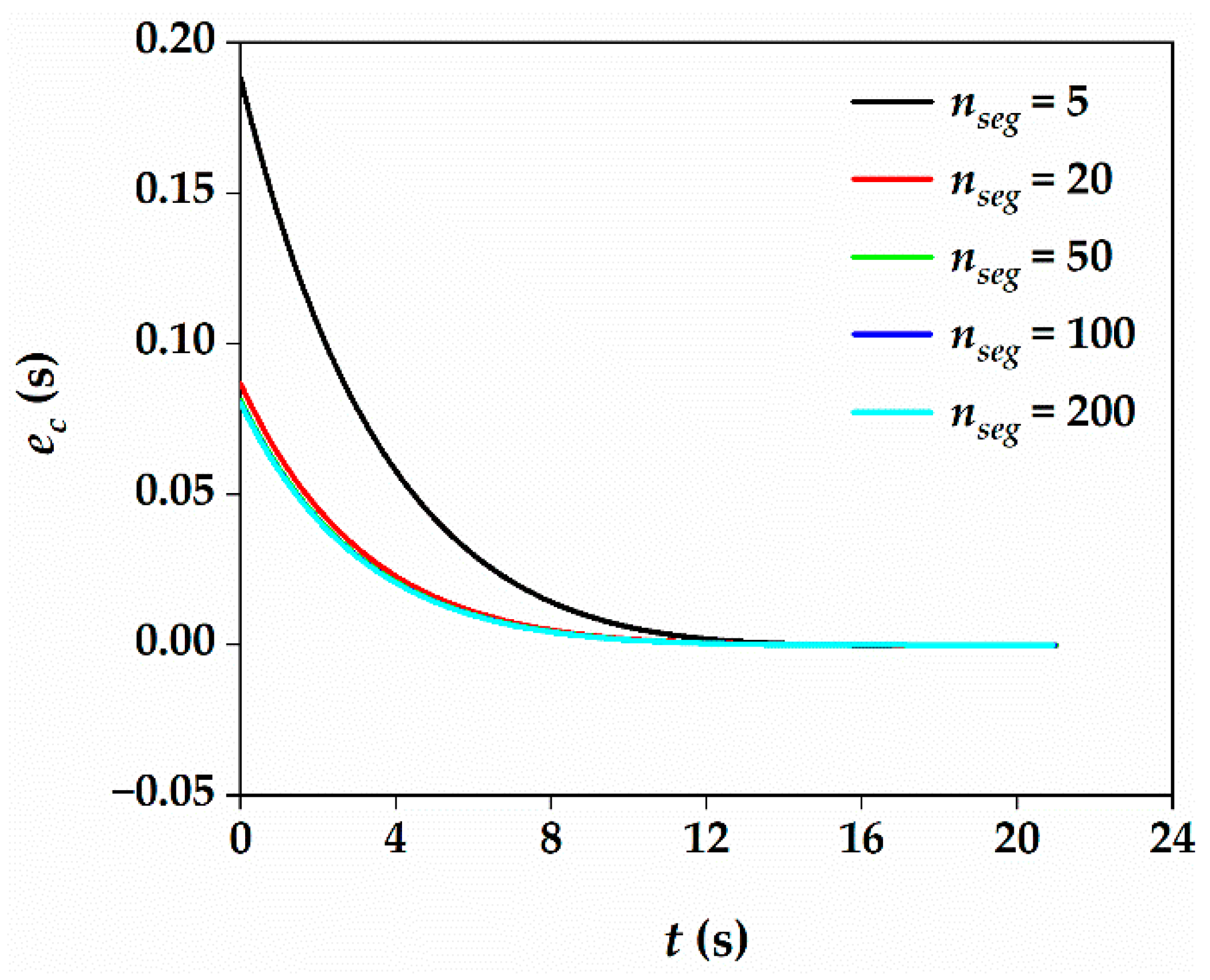
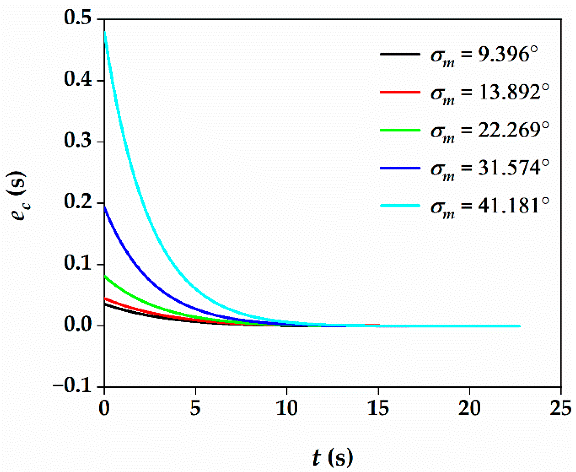
5.1. Verification of Three-Dimensional T_go Estimation Algorithm

To numerically solve (25) and (26) to obtain the estimate of t_go, an appropriate step size must be selected. In this study, the relative distance R is equally divided into n_seg segments, regardless of the current value of R. The number of segments n_seg will affect the estimation accuracy. In addition, the proposed t_go estimation algorithm is derived based on the small lead angle assumption; thus, it is necessary to analyze the influence of the lead angle on the estimation accuracy.

The coordinates of the stationary target are (4500, 0, 793.5) m. In addition to the parameters listed in Table 1, other relevant simulation parameters are V_p = 250 m/s, R = 4862.6 m, φ_v = 0°, θ_L = −20°, and φ_L = −10°. To simulate the effect of different n_seg, θ_v = 0°, and n_seg = 5, 20, 50, 100, and 200. The simulation results are shown in

Table 2. Simulation results under different n_seg.

nseg	Tf (s)	Te (s)	ecm (s)	ecm/Tf (%)
5	21.007	21.196	0.189	0.900
20	21.007	21.094	0.087	0.414
50	21.007	21.088	0.081	0.386
100	21.007	21.088	0.081	0.386
200	21.007	21.087	0.080	0.381

and Figure 2. To simulate the effect of different initial lead angles, n_seg = 50, and θ_v = −20°, −10°, 0°, 10°, and 20°, respectively. The value of lead angle σ_m can be obtained from (8) and (17). The simulation results are shown in

Table 3. Simulation results under different initial lead angles.

θv (°)	σm (°)	Tf (s)	Te (s)	ecm (s)	ecm/Tf (%)
−20	9.396	20.594	20.630	0.036	0.175
−10	13.892	20.644	20.689	0.045	0.218
0	22.269	21.007	21.088	0.081	0.386
10	31.574	21.692	21.885	0.193	0.890
20	41.181	22.719	23.198	0.479	2.108

and Figure 3. In Table 2 and Table 3, the real flight time T_f, the estimated flight time T_e, the maximum estimation error e_cm, and the maximum estimation error percentage are listed.

Table 2 shows that increasing n_seg can improve the estimation accuracy of t_go. If n_seg ≥ 20, the maximum estimation error is less than 0.1 s, and the estimation algorithm achieves a high accuracy. In addition, if n_seg ≥ 50, increasing n_seg will not improve the estimation accuracy markedly. Therefore, considering the computational efficiency and estimation accuracy, we set n_seg = 50. Figure 2 shows that the estimation error decreases monotonically with respect to t because the estimation algorithm is derived based on the small lead angle assumption, and the lead angle decreases monotonically under the PNG law. With a decreasing lead angle, the accuracy of the estimation algorithm gradually increases.

Table 3 and Figure 3 show that the estimation error decreases monotonically, and the larger the initial lead angle is, the larger the maximum estimation error. If the initial lead angle is less than 30°, the maximum estimation error is less than 0.9%, and the estimation algorithm can ensure good estimation accuracy. If the initial lead angle reaches 41.18°, the maximum estimation error is greater than 2.1%. We can infer that if the initial lead angle continues to increase, the estimation accuracy continues to decrease. Therefore, to ensure the accuracy of the estimation algorithm, we should ensure that the lead angle is less than 40°. This condition can be satisfied for the terminal guidance phase of the guided projectile.

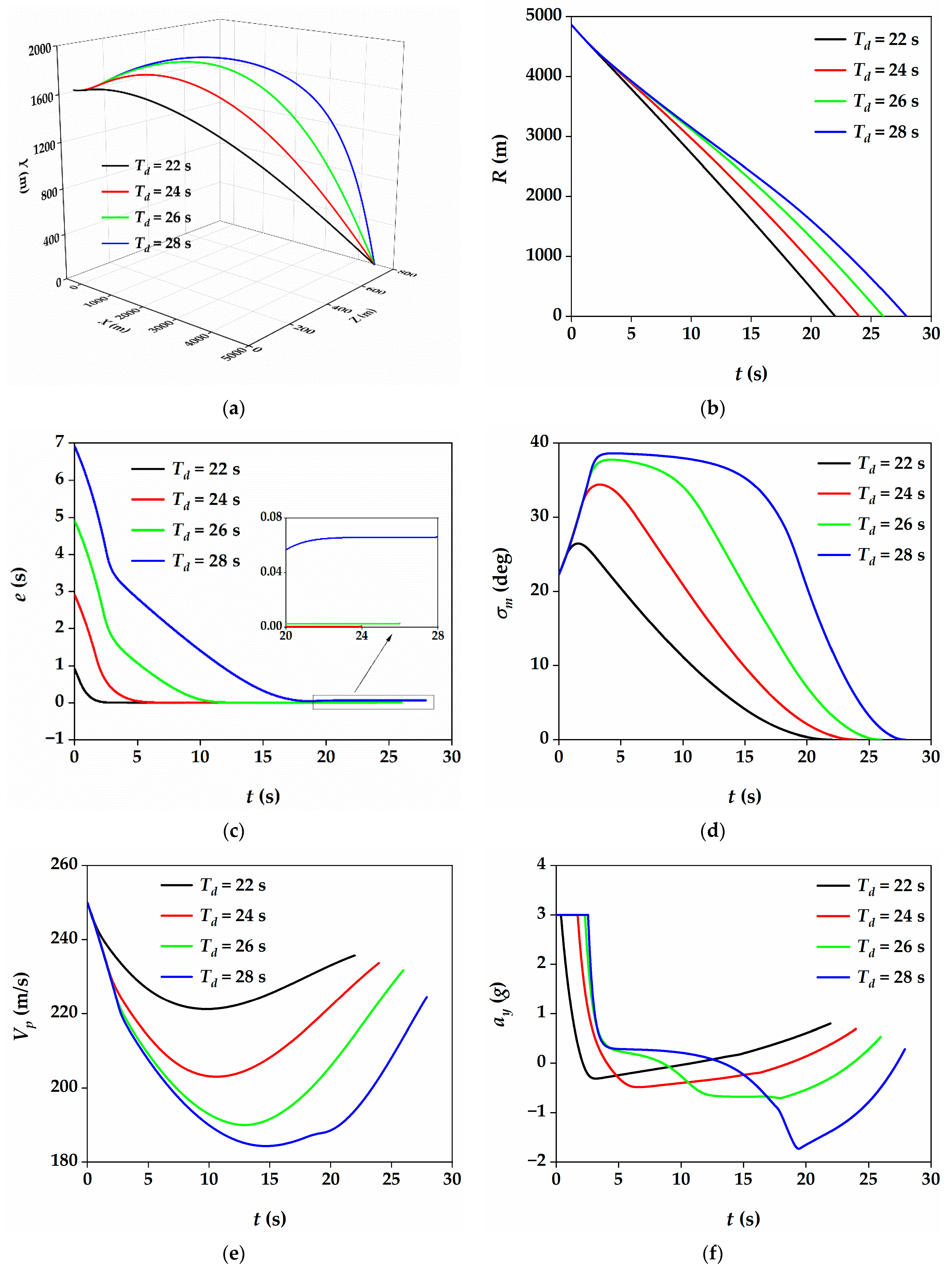
5.2. Performance of the Three-Dimensional ITCG Law under Different Designated Times

In this subsection, to verify the performance of the proposed ITCG law under different designated impact times T_d, numerical simulations are performed. The coordinates of the stationary target are (4500, 0, 793.5) m. In addition to the parameters listed in Table 1, other relevant simulation parameters are V_p = 250 m/s, R = 4862.6 m, θ_v = 0°, φ_v = 0°, θ_L = −20°, φ_L = −10°, and n_seg = 50. The coefficients related to ITCG laws (41) and (42) are R_ce = 1981.3 m, α = 0.5, k₁ = 50, k₂ = 0.15, and k₃ = 5. The allowable maximum FOV angle σ_max = 40°. The designated impact times T_d = 22 s, 24 s, 26 s, and 28 s, respectively. The termination condition of the simulation is that the relative distance is less than 0.5 m. The simulation results are shown in Figure 4.

The flight trajectory of the guided projectile is shown in Figure 4a. Figure 4b shows the variation of relative distance R with t, and we can see that the guided projectile can intercept the target under the four cases. Figure 4c shows the variation of impact time error e concerning t, where the larger the designated impact time T_d is, the longer the convergence time of e. In addition, the terminal impact time error is less than 0.1 s, which means that the proposed ITCG law can effectively adjust the flight time of the guided projectile. Figure 4d shows the change in the lead angle with respect to t. The FOV constraint can thus be achieved in all four cases. Figure 4e shows the variation in velocity, where the larger T_d is, the lower the final velocity. The variations in a_y and a_z are shown in Figure 4f,g, respectively. The guidance command is continuous, and the terminal guidance command is small.

5.3. Performance of the Three-Dimensional ITCG Law under Different FOV Constraints

In this subsection, numerical simulations are performed to verify the performance of the proposed ITCG law under different FOV constraints. The designated impact time T_d = 24 s. The allowable maximum lead angle is considered to be σ_max = 30°, 35°, and 40°. Other simulation parameters are the same as those in Section 5.2. The simulation results are shown in Figure 5.

Figure 5a shows the flight trajectory, and Figure 5b shows the variation of relative distance. It can be seen that the simulation terminates when R is less than 0.5 m, and the guided projectile can intercept the target under the three cases. The variation in the impact time error e with respect to t is shown in Figure 5c. The impact time error e eventually tends to 0 in all three cases, where the larger the value of σ_max is, the faster the convergence of e. This phenomenon is because the effect of σ_max on the biased term (37) is concentrated on the function δ. The larger the σ_max, the larger the function δ, and the larger the value of the biased term, thereby reducing the impact time error faster. Figure 5d shows the change in lead angle, and the proposed ITCG law can meet the FOV constraint. The profile of projectile velocity is shown in Figure 5e. Little difference in terminal velocity is found between these three cases. The profiles of a_y and a_z are shown in Figure 5f,g, respectively. The acceleration constraint can be satisfied, the guidance command is continuous, and the terminal guidance command is small.

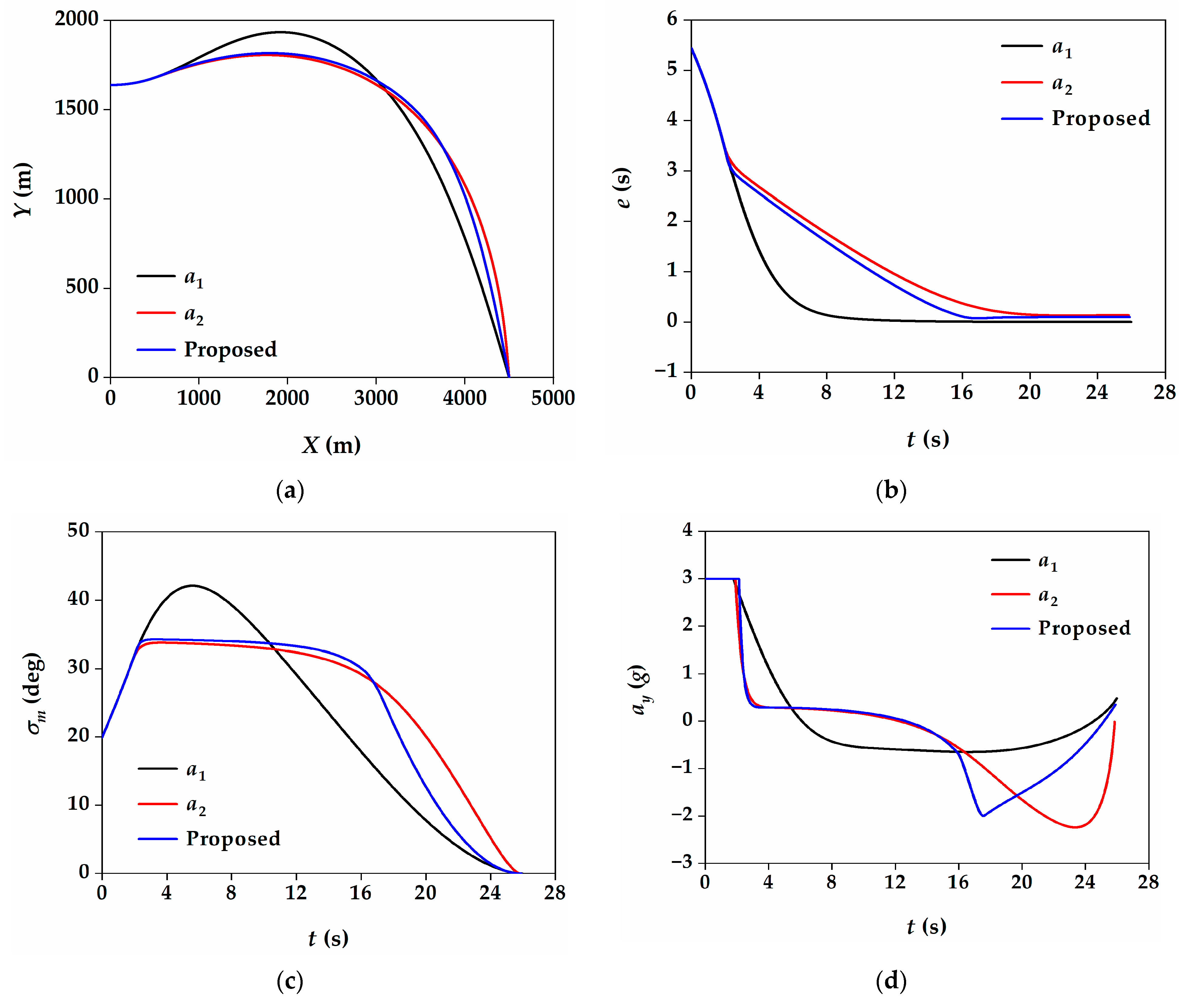
5.4. Compared with Other Guidance Laws

The core idea of this study is similar to that of [21,22]: the t_go estimation algorithm under the PNG law is first derived, and then, the ITCG law is designed based on the BPNG structure. Note that the ITCG law in [21] is designed for hypersonic bank-to-turn vehicles, while the ITCG law in [22] is designed for conventional missiles. Therefore, the ITCG law in [22] is selected for comparison in this study. For convenience, the ITCG law in [22] is denoted as a₁, which is designed only for the longitudinal plane and is described as follows:

$$a_1=-\frac{N}{R}{V}_p^2\sin {\theta }_m+g\cos {\theta }_v+k_1\delta (1-R/R_0)|e{|}^{0.5}\mathrm{sgn}(e)$$

(43)

In (43), the function δ(·) is the same as in (39). The guidance law a₁ cannot guarantee the FOV constraint, but by introducing the function of the lead angle into a₁, we can obtain a new guidance law a₂ that satisfies the FOV constraint. The modified guidance law a₂ is as follows:

$$a_2=-\frac{N}{R}{V}_p^2\sin {\theta }_m+g\cos {\theta }_v+k_1\delta (1-R/R_0)\delta (\frac{{\sigma }_m}{{\sigma }_{\max }})|e{|}^{0.5}\mathrm{sgn}(e)$$

(44)

In this subsection, numerical simulations are performed to compare the performance of a₁ and a₂ with the proposed ITCG law in two-dimensional engagement. Two simulation scenarios are considered in this subsection. In scenario 1, T_d = 24 s; in scenario 2, T_d = 26 s. The coordinates of the stationary target are (4500, 0, 0) m. Other simulation parameters are considered to be V_p = 250 m/s, R = 4788.9 m, θ_v = 0°, φ_v = 0°, θ_L = −20°, φ_L = 0°, and n_seg = 50. The allowable maximum guidance command a_max = 3 g, and the allowable maximum FOV angle σ_max = 35°. In the simulation of the proposed ITCG law, R_ce = 1981.3 m. The other coefficients are shown in

Table 4. Simulation coefficients under different ITCG laws.

ITCG Laws	Scenario 1	Scenario 2
a1	k1 = 20, k3 = 5	k1 = 20, k3 = 5
a2	k1 = 50, k2 = 5, k3 = 5	k1 = 50, k2 = 5, k3 = 5
Proposed	k1 = 50, k2 = 0.15, k3 = 5	k1 = 80, k2 = 0.15, k3 = 5

, and the simulation results are shown in

Table 5. Simulation results under different ITCG laws.

ITCG Laws	Scenario 1		Scenario 2
	Tf (s)	E (m2/s3)	Tf (s)	E (m2/s3)
a1	23.995	1982	25.995	3040
a2	23.998	2078	25.863	4543
Proposed	23.997	2090	25.899	3542

and Figure 6 and Figure 7. The real flight time T_f and the control energy consumption $E=\int a_y^{2}dt$ are listed in Table 5. The termination condition of the simulations is that the relative distance is less than 0.5 m.

Figure 6 and Table 5 show that in scenario 1, the impact time and FOV constraints can be achieved under the three ITCG laws. The performance of a₂ and the proposed ITCG law is nearly identical under scenario 1. The maximum lead angle is the largest, and the control energy consumed is the smallest under guidance law a₁. Figure 7 and Table 5 show that all three guidance laws can realize the impact time constraint, while only a₁ cannot ensure that the FOV constraint is met. We can also see that compared with ITCG law a₂, the impact time error is smaller and the control energy assumption is lower under the proposed ITCG law. Therefore, if the FOV constraint is not considered or the impact time error is small, the ITCG law a₁ can be selected to reduce the consumption of control energy; if the FOV constraint needs to be considered or the impact time error is large, the proposed ITCG law is better. In addition, the most important advantage of the proposed ITCG law is that it can be used for three-dimensional engagement, while the guidance laws a₁ and a₂ cannot.

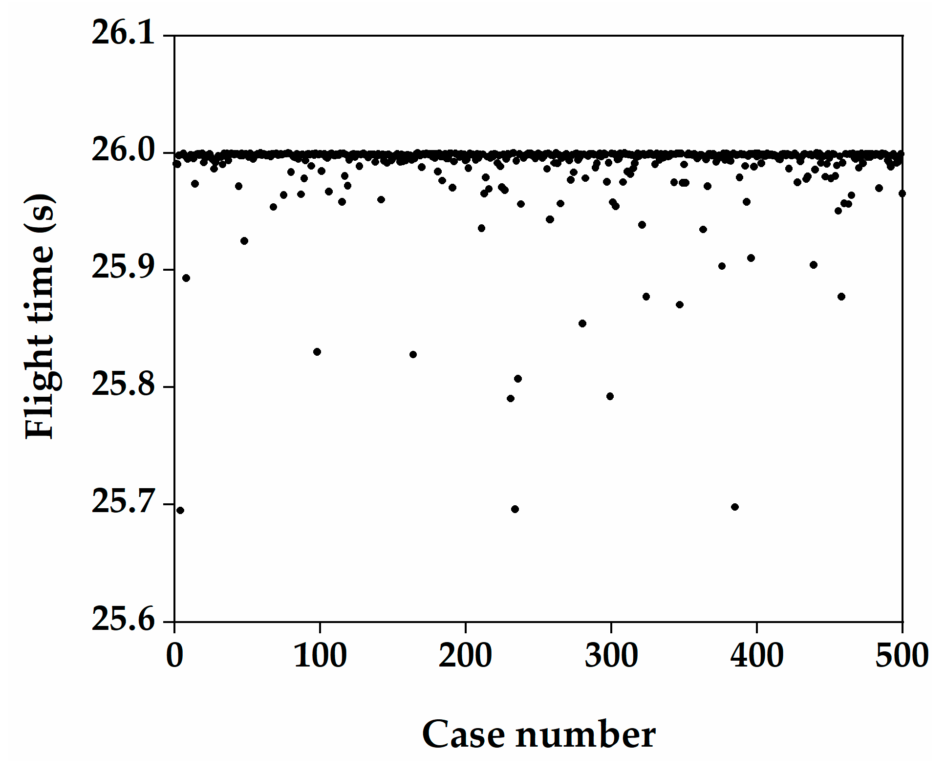
5.5. Monte Carlo Simulation

In Section 5.2 and Section 5.3, we verified the effectiveness of the proposed ITCG law in impact time control and FOV constraint. For guided projectiles of the same type, the mass and aerodynamic coefficients are not exactly the same due to manufacturing errors, which may affect the accuracy of the time-to-go estimation algorithm and the proposed ITCG law. Therefore, Monte Carlo simulations are employed to demonstrate the performance of the proposed method in this subsection.

In addition to the perturbation of mass and aerodynamic coefficients, the perturbation of initial parameters (V_p, θ_v, φ_v, θ_L, φ_L) is also considered. The perturbation parameters are subject to uniform distribution, and the value range is shown in

Table 6. Monte Carlo simulation parameters.

Parameter	Value	Parameter	Value
m (kg)	37.27 ± 0.1	CD0	0.352 ± 0.035
CLα	13.365 ± 1.337	Vp (m/s)	250 ± 10
θv (°)	0 ± 5	φv (°)	0 ± 5
θL (°)	−20 ± 5	φL (°)	−10 ± 5

. The designated impact times T_d = 26 s, and the allowable maximum FOV angle σ_max = 40°. The coefficients related to ITCG laws (41) and (42) are R_ce = 1981.3 m, α = 0.5, k₁ = 60, k₂ = 0.15, and k₃ = 5. In order to reduce the simulation time, we take H = 0.01 s and n_seg = 30. Five-hundred-run Monte Carlo simulations are carried out, and the simulation results are shown in Figure 8.

In Figure 8, it can be seen that only 13 of the 500 simulations have an impact time error larger than 0.1 s. The maximum impact time error in the 500-run Monte Carlo simulations is 0.305 s. Therefore, the proposed method can effectively adjust the flight time of guided projectile. In addition, we can see that for the specified T_d, the flight time is essentially not larger than T_d. There are two reasons for this phenomenon. One is that the proposed time-to-go estimation algorithm has good estimation accuracy. Another is that the flight time of the projectile under PNG law is less than T_d, and the biased term has been shown to be able to adjust the flight time. Once the impact time error converges to 0, the biased term also converges to 0, and thus the flight time will not continue to increase.

6. Conclusions

In this study, the problem of three-dimensional impact time control guidance while considering FOV constraints and velocity variations is addressed. Based on the simplified guidance model, a new time-to-go estimation algorithm with the three-dimensional PNG law is deduced. Then, the effect of the biased term on the projectile flight time is analyzed and described. Finally, based on the analysis results, an ITCG law with the BPNG structure is designed. Simulation results show that the proposed time-to-go estimation algorithm achieves good estimation accuracy. The proposed ITCG law can determine impact time and FOV constraints with time-varying velocities. Compared with existing methods, the proposed method achieves better performance when considering the FOV constraint and can be used in three-dimensional engagement. The results of this study provide a preliminary theoretical basis for the engineering implementation of multi-projectile salvo attacks. In the follow-up research, the biased terms can be added to both the normal and lateral planes to achieve optimal control energy consumption, and the terminal impact angle constraint can also be considered.

References

1. Jeon, I.S.; Lee, J.I.; Tahk, M.J. Impact-time-control guidance law for anti-ship missiles. IEEE Trans. Control. Syst. Technol. 2006, 14, 260–266. [Google Scholar] [CrossRef]
2. Jeon, I.S.; Lee, J.I.; Tahk, M.J. Homing Guidance Law for Cooperative Attack of Multiple Missiles. J. Guid. Control. Dyn. 2010, 33, 275–280. [Google Scholar] [CrossRef]
3. Harl, N.; Balakrishnan, S.N. Impact Time and Angle Guidance With Sliding Mode Control. IEEE Trans. Control. Syst. Technol. 2012, 20, 1436–1449. [Google Scholar] [CrossRef]
4. Zhu, J.W.; Su, D.L.; Xie, Y.; Sun, H.F. Impact time and angle control guidance independent of time-to-go prediction. Aerosp. Sci. Technol. 2019, 86, 818–825. [Google Scholar] [CrossRef]
5. Chen, Y.D.; Wang, J.N.; Wang, C.Y.; Shan, J.Y.; Xin, M. Three-Dimensional Cooperative Homing Guidance Law with Field-of-View Constraint. J. Guid. Control. Dyn. 2020, 43, 389–397. [Google Scholar] [CrossRef]
6. Chen, Z.Y.; Chen, W.C.; Liu, X.M.; Cheng, J. Three-dimensional fixed-time robust cooperative guidance law for simultaneous attack with impact angle constraint. Aerosp. Sci. Technol. 2021, 110, 106523. [Google Scholar] [CrossRef]
7. Zhang, Y.A.; Wang, X.L.; Wu, H.L. Impact time control guidance law with field of view constraint. Aerosp. Sci. Technol. 2014, 39, 361–369. [Google Scholar] [CrossRef]
8. Chen, X.T.; Wang, J.Z. Nonsingular Sliding-Mode Control for Field-of-View Constrained Impact Time Guidance. J. Guid. Control. Dyn. 2018, 41, 1214–1222. [Google Scholar] [CrossRef]
9. Kim, H.G.; Lee, J.Y.; Kim, H.J.; Kwon, H.H.; Park, J.S. Look-Angle-Shaping Guidance Law for Impact Angle and Time Control With Field-of-View Constraint. IEEE Trans. Aerosp. Electron. Syst. 2020, 56, 1602–1612. [Google Scholar] [CrossRef]
10. Lee, S.; Cho, N.; Kim, Y. Impact-Time-Control Guidance Strategy with a Composite Structure Considering the Seeker’s Field-of-View Constraint. J. Guid. Control. Dyn. 2020, 43, 1566–1574. [Google Scholar] [CrossRef]
11. Mukherjee, D.; Kumar, S.R. Field-of-View Constrained Impact Time Guidance Against Stationary Targets. IEEE Trans. Aerosp. Electron. Syst. 2021, 57, 3296–3306. [Google Scholar] [CrossRef]
12. Ma, S.; Wang, X.G.; Wang, Z.Y. Field-of-View Constrained Impact Time Control Guidance via Time-Varying Sliding Mode Control. Aerospace 2021, 8, 251. [Google Scholar] [CrossRef]
13. Zhou, J.; Wang, Y.; Zhao, B. Impact-Time-Control Guidance Law for Missile with Time-Varying Velocity. Math. Probl. Eng. 2016, 2016, 7951923. [Google Scholar] [CrossRef]
14. Wen, L.; Ping, L.; Liang, W.; Huabin, L.; Jie, G. Three-dimensional guidance law of impact-time-control under time-varying velocity. In Proceedings of the 2018 IEEE CSAA Guidance, Navigation and Control Conference (CGNCC), Xiamen, China, 10–12 August 2018; pp. 1–6. [Google Scholar]
15. Yan, X.H.; Kuang, M.C.; Zhu, J.H. A Geometry-Based Guidance Law to Control Impact Time and Angle under Variable Speeds. Mathematics 2020, 8, 1029. [Google Scholar] [CrossRef]
16. Zhu, C.H.; Xu, G.D.; Wei, C.Z.; Cai, D.Y.; Yu, Y. Impact-Time-Control Guidance Law for Hypersonic Missiles in Terminal Phase. IEEE Access 2020, 8, 44611–44621. [Google Scholar] [CrossRef]
17. Jiang, Z.Y.; Ge, J.Q.; Xu, Q.Q.; Yang, T. Impact Time Control Cooperative Guidance Law Design Based on Modified Proportional Navigation. Aerospace 2021, 8, 231. [Google Scholar] [CrossRef]
18. Snyder, M.; Qu, Z.H.; Hull, R.; Prazenica, R. Quad-Segment Polynomial Trajectory Guidance for Impact-Time Control of Precision-Munition Strike. IEEE Trans. Aerosp. Electron. Syst. 2016, 52, 3008–3023. [Google Scholar] [CrossRef]
19. Tekin, R.; Erer, K.S.; Holzapfel, F. Adaptive Impact Time Control Via Look-Angle Shaping Under Varying Velocity. J. Guid. Control. Dyn. 2017, 40, 3247–3255. [Google Scholar] [CrossRef]
20. Guo, Y.H.; Li, X.; Zhang, H.J.; Cai, M.; He, F. Data-Driven Method for Impact Time Control Based on Proportional Navigation Guidance. J. Guid. Control. Dyn. 2020, 43, 955–966. [Google Scholar] [CrossRef]
21. Wang, J.W.; Zhang, R. Terminal Guidance for a Hypersonic Vehicle with Impact Time Control. J. Guid. Control. Dyn. 2018, 41, 1790–1798. [Google Scholar] [CrossRef]
22. Sun, G.X.; Wen, Q.Q.; Xu, Z.Q.; Xia, Q.L. Impact time control using biased proportional navigation for missiles with varying velocity. Chin. J. Aeronaut. 2020, 33, 956–964. [Google Scholar] [CrossRef]
23. Wang, X.H.; Tan, C.P. 3-D impact angle constrained distributed cooperative guidance for maneuvering targets without angular-rate measurements. Control. Eng. Pract. 2018, 78, 142–159. [Google Scholar] [CrossRef]
24. Chen, Q.; Wang, Z.; Chang, S.; Fu, J. Multiphase trajectory optimization for gun-launched glide guided projectiles. Proc. Inst. Mech. Eng. Part G J. Aerosp. Eng. 2015, 230, 995–1010. [Google Scholar] [CrossRef]
25. Song, S.-H.; Ha, I.-J. A Lyapunov-like approach to performance analysis of 3-dimensional pure PNG laws. IEEE Trans. Aerosp. Electron. Syst. 1994, 30, 238–248. [Google Scholar] [CrossRef]
26. He, S.; Lee, C.-H.; Shin, H.-S.; Tsourdos, A. Optimal three-dimensional impact time guidance with seeker’s field-of-view constraint. Chin. J. Aeronaut. 2021, 34, 240–251. [Google Scholar] [CrossRef]
27. Zhang, D.C.; Xia, Q.L.; Wen, Q.Q.; Zhou, G.Q. An Approximate Optimal Maximum Range Guidance Scheme for Subsonic Unpowered Gliding Vehicles. Int. J. Aerosp. Eng. 2015, 2015, 389751. [Google Scholar] [CrossRef] [Green Version]
Figure 1. Three-dimensional homing engagement geometry.
Aerospace 09 00202 g001
Figure 2. Simulation results under different nseg.
Aerospace 09 00202 g002
Figure 3. Simulation results under different initial lead angles.
Aerospace 09 00202 g003
Figure 4. Simulation results under different Td. (a) Projectile flight trajectory; (b) relative distance; (c) impact time error; (d) lead angle; (e) velocity; (f) normal acceleration; (g) lateral acceleration.
Aerospace 09 00202 g004aAerospace 09 00202 g004b
Figure 5. Simulation results under different FOV constraints. (a) Projectile flight trajectory; (b) relative distance; (c) impact time error; (d) lead angle; (e) velocity; (f) normal acceleration; (g) lateral acceleration.
Aerospace 09 00202 g005aAerospace 09 00202 g005b
Figure 6. Comparison of simulation results under scenario 1. (a) Projectile flight trajectory; (b) impact time error; (c) lead angle; (d) normal acceleration.
Aerospace 09 00202 g006
Figure 7. Comparison of simulation results under scenario 2. (a) Projectile flight trajectory; (b) impact time error; (c) lead angle; (d) normal acceleration.
Aerospace 09 00202 g007
Figure 8. Flight time under Monte Carlo simulation.
Aerospace 09 00202 g008