Abstract
Nowadays, with the increase of the thrust-to-weight ratio of the aero engines, the high aerodynamic load has made corner separation an issue for axial compressors. The complex three-dimensional flow field makes it challenging to suppress the corner separation, especially considering the performance at multi-working conditions. To suppress the corner separation and reduce loss, the investigation in this paper proposed a new parametric suction side corner profiling method, which includes few variables but enables the flexible variation of the shape. A bi-objective auto-optimization design process for the corner profiling was carried out on a high-load linear compressor cascade, with the companion of end wall and blade profiling. The aim was to investigate the effective flow control rules for the corner separation and practical design guidelines for its geometry under multiple working conditions. The numerical results identified that the suction side corner profiling brings a much more dominant effect to corner separation than end wall profiling and blade profiling. The most critical flow control rule is to accelerate the climbing second flow on the bottom of the suction surface to suppress the reverse trend of the boundary layer and further relieve the corner separation. In addition, the design point and near-stall point have different well-fitting thicknesses and axial positions. A medium value between the design and near-stall well-fitting parameters will make the suction side corner profiling a best-matching case for a medium inflow condition and adequate performance at a range of conditions.
1. Introduction
Modern compressors are commonly designed with higher aerodynamic loads to increase the thrust-to-weight ratio of aero engines. As a result, the high streamwise/pitch-wise pressure gradient induces significant three-dimensional corner separation. Among them, is the corner separation that significantly damages the performance of compressors. The dissipation loss of its low-energy separation fluid would reduce the efficiency. In some instances, the blockage of the separation flow even challenges the stability of the compressor.
The development of corner separation is closely related to the load of the compressor. In particular, when there is a thick boundary layer in a high-load compressor blade row, the low-energy fluid that accumulates at the SS corner or even climbing on the SS will reach a significant level and form a sizeable reverse flow region. The corner separation thus induces remarkable end wall loss. According to Lakshminarayana’s research [1], the end wall loss could reach 35% of the total when the corner stall happens, even for a large aspect ratio cascade (AR = 4.3). This indicates the significance of the analysis and control of corner separation for the performance improvement of compressors.
Unlike the two-dimensional separation flow, the occurrence of corner separation is not only influenced by the fluid viscosity and the inverse pressure gradient but is also closely related to the secondary flow motion. Any change in the secondary flow at the SS and the end wall region will affect its development. A notable work by Lei [2] employed the dimensional analysis and proposed ten parameters for evaluating separation, i.e., inlet Mach number, Reynolds number, boundary layer thickness, inflow/outflow angle, blade aspect ratio, et al. However, considering the actual operation of a compressor stage at a particular design speed, it should be only the boundary layer thickness and the inflow angle that vary significantly from the design point to the off-design point. The variation of boundary layer thickness is generally caused by the growth of end wall blockage due to the throttling. According to the experimental results of Zhang [3], a thicker incoming boundary layer enlarges the corner separation and increases loss but negligibly affects the topology of separation flow. So, boundary layer thickness changes the level of separation rather than its structure. In comparison, the inflow angle is more influential to the corner separation. Studies on the cascade by Ma [4] and Li [5] both showed a positive correlation between the growth of inflow angle and separation loss. In addition, in capturing the physical mechanisms associated with corner separation, Gbadebo [6] analyzed the topology of limiting streamlines on a high-load compressor cascade. The result indicates that corner separation extends on the SS with a complex variation of critical points and streamlines when the incidence increases. Lewin [7] studied the variation of end wall secondary flow with the increase of the inflow angle and identified the topology of corner separation could vary at the inception of the corner stall. Besides, in the experimental research of Zambonini [8], the corner separation shows its unstable nature at a high inflow angle. The corner separation presents a high-energy and low-frequency size switch between massively open and almost closed, along with complex topological changes. All of the above clearly shows the close relationship between the inflow angle and the topology of the corner separation. Considering the inflow angle is mainly decided by the mass flow rate, it indicates that the flow structure of corner separation may be re-organized when the compressor’s operating condition changes, thus maybe requiring distinct flow control methods.
To improve the performance of the high-load compressor, several promising control techniques have been proposed and validated. The commonly used passive flow control techniques include three-dimensional blading [9], profiled end wall [5], vortex generator [10], et al. All of them control the corner separation by working on the “system” of secondary flow from the end wall to the SS, within which the suction surface (SS) corner is believed to be a critical region because of its direct influence on the corner separation. The design of this SS corner profiling thus became an issue of long-term research.
According to a review of the published literature, the most influential research into the SS corner design can be broadly separated into two categories. One of them is known as the “lean blade,” which means to vary the dihedral between the SS and the hub end wall to an obtuse angle or acute angle by moving the blade section perpendicular to the direction of the chord line in the end wall region. The use of the lean blade can date back to the 1960s [11]. Much research in the past decades has shown how the dihedral of lean blade affects the corner separation. Breugelmans started an experimental study on a compressor cascade [12], indicating that the secondary flow in the acute angle between the suction surface and end wall develops into a large corner stall. In contrast, in the obtuse angle, the secondary flow is suppressed. Later research by Sasaki and Breugelmans [13] revealed that the obtuse dihedral angle would lead to unloading near the end wall and overloading around the midspan. Besides, the obtuse dihedral angle also creates a higher spanwise pressure gradient on the SS and prevents an accumulation of low-energy fluid near the end wall. Both effects are beneficial in delaying the onset of the corner separation and reducing the loss in the end wall region, but inevitably increase loss in the mid-span region. The follow-up numerical and experiment research of Roy [14], Denton [15,16], Gallimore [17], and Talyor [18], et al. bring more details in the flow field; however, all comment on the effect of the blade loading and the spanwise pressure gradient mentioned by Breugelmans. This confirms that the lean blade is geometrically near the end wall region but actually affects the overall span range of the compressor passage.
Next to the lean blade, another method of SS corner profiling is to fill up the dihedral between the SS and hub end wall. Compared with the well-known lean blade, the fill-up of the SS corner will not vary the stacking of the blade element too much nor significantly redistribute the load of the blade over the spanwise direction. Ji et al. [19,20] proposed the BBEW method to blend the blade surfaces and end wall in the turbomachinery, generating a transition surface in the spanwise extension of boundary layer thickness to reduce the streamwise pressure gradient of the rear passage of the compressor to suppress the corner separation. Li et al. [21] applied a program that controls the shape of corner profiling by Bezier curves. The program can adjust the maximum thickness of the transient surface and its corresponding streamwise position. The research found that the corner profiling with the maximum thickness in the first 25% chord of the blade passage would reduce the separation loss in multiple working conditions. SS corner profiling suppresses corner separation by forming a transition surface from the end wall to the SS. Then the end wall secondary flow can be driven smoothly to the SS and turned downstream, thus energizing the boundary layer and suppressing the reverse flow. Later research [22] tested SS corner profiling with different maximum thickness and streamwise positions, finding that the maximum thickness should not be placed near the trailing edge, and there is an optimum value for the thickness. Otherwise, the corner profiling would deteriorate corner separation under large incidence. Reutter et al. [23] combined the profiling on the SS corner and the end wall. They designed the profiling shape using an optimization program to reduce loss in multiple working conditions. The recent research of Meng [24] also started an optimization design for the combined profiling on the SS corner and the end wall. The study proposed a simplified parameterization method for the end wall region to control the cross-passage pressure gradient and further improve the performance of the corner profiling.
Overall, the above studies have well illustrated the complex mechanism of corner separation and the progress in controlling the SS corner flow. However, they also reveal the problems that remain unsettled.
First, studies on the corner separation show the possible variation flow structure from the design point to the off-design point, indicating that the required flow control method may vary along with the compressor’s operating range. That brings a challenge to the application of SS corner profiling. This is because the existing design method generally relies on a particular formula to generate the structure, thus making the geometry lack sufficient design space to accommodate suitable aerodynamic shapes for a wide working range of compressors. Although the published studies show some specific results that are well-performing at different inflow conditions, the effective flow control rules, especially for their applicability under multiple working conditions, and the co-effects between the SS corner profiling are not yet understood.
Second, the above investigation indicates that corner separation develops under the combined effect of the secondary flow in the end wall, SS, and the corner region. So, in addition to the corner profiling, the control of the secondary flow in the end wall area and on the SS may bring further benefits. According to the published research, end wall profiling is one of the most effective ways to control the end wall secondary flow. The recent investigation of end wall profiling generally carried out an optimization design on a parametric end wall surface over dozens of control points [25]. Experimental and numerical results have confirmed that the control of corner separation is closely associated with the variation of the end wall pressure field [25,26,27]. However, few of these have reached an agreement on the flow control rules. As for the SS profiling, here, the only focus is on those not varying the stacking laws of the blades. The relevant research for SS profiling is not as much as for the end wall profiling. Although SS profiling does not always work well, and some research found it even causes an increase in loss [28], it is yet confirmed that SS profiling can influence the separation flow by varying the local pressure gradient, and thus is able to improve the flow field [29,30,31] locally. Therefore, the previous research indicates combining SS corner profiling with end wall profiling, and that SS profiling may be a promising way to further increase the performance of SS corner profiling. So, more research is worthy of being carried out to understand their advantages, shortcomings, and interactions when working together for better overall performance.
This paper mainly focuses on the fill-up type of SS corner profiling to control the corner separation without altering the spanwise stacking law and blade loading. Based on the previous research, this paper’s investigation proposes a new parametric SS corner profiling method that applies fewer profiling parameters but enables more flexible shape variation. This study investigates the SS corner profiling combined with end wall profiling and SS profiling to maximize its performance under multiple working conditions. The profiling is designed utilizing the auto-optimization and then analyzed with the aim to:
- Verify the effectiveness of adding the end wall profiling and the SS profiling in the control of corner separation, understand how they interact with each other, and contribute to reducing loss.
- Identify the most effective flow control rules and design guidelines to reduce the loss when corner separation develops to different levels due to the variation of the working conditions.
2. Methodology
2.1. Parameterization of the SS Corner Profiling
For the profiling on the SS corner, Figure 1 introduces the parameterization using the geometry model of a compressor cascade for convenience. A Cartesian plane is defined using x, y, and z axes pointing in the axial direction, circumferential direction, and spanwise direction. In Figure 1a, The Z0-plane means the baseline end wall plane, and the X-plane means an arbitrary plane perpendicular to the Z0-plane and x-axis. The SS corner profiling is defined as in Figure 1b, i.e.,
where ySS,baseline means the circumferential coordinate of the baseline SS geometry, and ySS represents the associate coordinate after profiling. Δy means the variation of the y coordinate of the SS due to the profiling. Δy is defined by the superposition of three sinusoidal functions, i.e.,

Figure 1.
Parameterization of the SS corner profiling. (a) Three-dimensional sketch of the SS corner profiling; (b) definition of the geometry.
Some preliminary profiling works supported that the three sinusoidal functions in Equations (3)–(5) should choose 2Ca, 0.5Ca, and 1.5Ca for their periods, respectively, as shown in Figure 1b. Each sinusoidal function defines two profiling variables, i.e., amplitude (ωi) and initial phase (γi). Additionally, when calculating the value of Δy, a smooth function, i.e., Smooth(x), has to be applied to the sum of the three sinusoidal functions to ensure a smooth transition at the LE and TE. In this study, the smooth function is defined as
Function F(z) in Equation (1) is a 3-order polynomial function in the spanwise direction defined by
where a1, a2, and a3 are all constants. As is shown in Figure 1a, the value of F equals one at the original hub plane (z = 0) and zero at the border of the boundary layer (z = δ). So, the variation of the SS in the hub corner region can smoothly change from Δy at the hub end wall to the SS.
In total, the new SS corner profiling method employs a flexible hub-section SS and a fixed spanwise transition rule. The SS corner profiling uses only six variables but can generate the shape of single-hump, dual-hump, or even waviness. The variation of the six variables will change the outline of the blade’s hub-section between −2.5%C and + 7.0%C in the circumferential direction and generate a smooth transition surface between the end wall and blade surface. Compared with the previously proposed corner profiling method, which applies a fixed algorithm with a single-hump of thickness over streamwise, the new approach enables more flexible shape variation. It thus is more applicable for both application and investigation.
2.2. Parameterization of the SS Profiling and End Wall Profiling
As a companion to the SS corner profiling, the SS and end wall profiling employ the traditional method. The surface is parameterized with loft surfaces over a group of Bezier curves, thus becoming more controllable but requiring many more control variables. The reason for applying the traditional parametric method is that it has been testified as reliable by numerous published research studies. So, it would ensure the end wall and SS profiling reach the maximum design space and provide as much improvement to the performance of the SS corner profiling as possible.
The Bezier curves in the SS profiling are defined as Si (i = 1, 2, …7) within a specific spanwise range, as shown by the grey area in Figure 2. Each of the curves has a fixed spanwise position and can rise and fall in the circumferential direction under the control of 8 flexible nodes, according to
where Δyi represents the variation of the y coordinate relative to the baseline SS. A positive value of Δyi means the SS rises, and a negative value means the opposite. sj,i (j = 1–8; I = 1–7) means the rise of jth control nodes on the ith curve. All 56 variables enable the SS locally to vary from −2.5%C to +7.0%C in the circumferential direction with smooth joints to the LE and TE. Those of the end wall profiling are defined as shown by the yellow area in Figure 3. All Bezier curves are circumferentially parallel to the camber curve and similarly controlled by eight flexible nodes according to
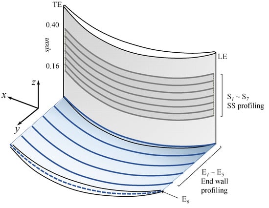
Figure 2.
Parameterization of the SS profiling and end wall profiling.

Figure 3.
The geometry parameters of the baseline cascade.
The difference is that E6 is dependent on E1 to make the end wall circumferentially periodic. Therefore, the end wall profiling is controlled by 40 variables in total. The surface will rise and fall within ±3.5%C while keeping smooth joints to the upstream, downstream, and adjacent end wall surface.
2.3. Baseline Compressor Cascade and the CFD Method
This study uses a typical high-load low-speed linear compressor cascade, as shown in Figure 3. The baseline blade geometry uses multiple circle arcs with a designed flow turning angle of 51° and diffusion factor (DF) of 0.5. Its solidity exceeds 2.0. Zhang [3] conducted a detailed experimental and numerical study on this cascade and has confirmed a significant three-dimensional corner separation occurring in the end wall region of this cascade. According to previous research [32], the cascade operates at the design point when the incidence (i) equals −1°, and the corner stall occurs when i exceeds +7°. Using linear cascade instead of an actual compressor ensures that the investigation of flow control will not be influenced by twisted blade sections, leakage flow, centrifugal force, and inlet boundary layer skew, but rather the inlet boundary layer and the secondary flow. So, only the most common features of a high-load compressor are considered, and the results will be universal.
The CFD results of the above cascade presented in this paper are computed using ANSYS CFX. Only a half-span of the single-passage cascade has been simulated with a free-slip boundary condition at the mid-span position to reduce the simulation time. The mesh is generated using NUMECA AutoGrid5. Figure 4 provides an overview of the computational domain. The inlet and outlet passages both use long extended “H” blocks. The former extends to 1.2Ca upstream of the LE, which is the location where experimental measurements were taken. The latter reaches 2.0Ca downstream of the TE to ensure adequate mixing of the outlet flow. The blade-to-blade flow surface employs refined nodes in the center with “O4H” topology to achieve a higher degree of orthogonality. The numbers of nodes in some important sections are also presented. The computational domain extends to 1.2Ca upstream of the LE, where the inlet velocity is taken during the experiment, and to 2.0Ca downstream of the TE for the uniformity of the outflow parameter. Considering the separation from the corner region, the mesh in the boundary layer region upon the blade surface and the end wall is further refined. The growth rate of mesh from the solid wall to the flow field is less than 1.1, and the y+ is less than 2 at the first level upon the solid wall.
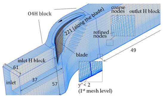
Figure 4.
Overview of the mesh.
The boundary condition is given according to the experiment result. The inlet boundary defines the static temperature and the inflow velocity. The thickness of the inlet boundary layer is about 12.5%span. The outlet boundary defines a uniform static pressure. The flow field of the cascade is calculated by solving the steady Reynolds-averaged Navier–Stokes (RANS) equations with the second-order upwind scheme. A preliminary numerical study tests several well-performing turbulence models for the separation flow, including the sst, k-ω, and the k-ε turbulence model. Finally, the most robust k-ε turbulence model is selected. Considering there is a transition of the SS boundary layer, the γ-θ transition model is also applied. The convergence criterion is set to a value of 1 × 10⁻⁶ for the RMS residual values. It should be noted that at the last operating condition of the compressor cascade, i.e., near the stall point, strong perturbations are often found in the actual flow field and lead to instability in the numerical model. However, in this case, the convergence history shows no significant perturbation, even near the stall point. Consequently, the steady simulation is still appropriate for the performance evaluation at the near stall condition. Local time stepping techniques are applied to speed-up convergence.
Figure 5 compares the experimental result of pitch averaged total pressure loss () and outflow angle with the CFD results calculated by three groups of mesh with different numbers of nodes, i.e., 0.4 million, 0.75 million, and 1.05 million. Compared with the CFD model of 0.45 million nodes and 1.05 million nodes, the result of 0.75 million nodes shows a subtle difference. It is seen that the quantitative errors of and flow angle due to the mesh size are less than 0.005 and 0.2°, respectively, which are almost negligible. So, the size of the three mesh groups is all adequate. More mesh nodes may lead to a higher resolution of the flow field in the later discussion. However, considering the time-consuming simulation in the optimization process, here we select the medium mesh size for the current study, i.e., the 0.75 million nodes.
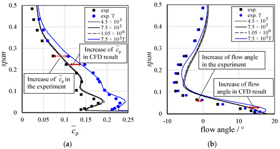
Figure 5.
The pitch-averaged performance at 40%Ca downstream of the TE at i = −1°. (a) Total pressure loss coefficient; (b) outflow angle.
The CFD results predict higher and outflow angle values than the experiment result. However, the calculated characteristics of the experimental curve (especially the “S” shape of the curve within the first 10% of span) and the location of the under-turning peak of the flow angle are almost the same as the experimental result. This indicates that the coupling effect of the corner separation and the hub cross-flow is well predicted. Besides, to further see how the CFD method performs in calculating the extension of corner separation, the experimental and CFD results with a thicker inlet boundary layer (thickness reaching 22.5%span) are also plotted labeled with “exp. T” and “7.5 × 10⁵ T”. The curves show that the CFD model calculates the effect of increased corner separation very well, both in magnitude and position of the changes in loss and flow angle, regardless of the absolute difference between the experimental and simulated values.
Figure 6 presents the numerical and experimental boundary flow on the SS. The oil- flow shows that the semi-saddle point (NS3) locates at 0.1Ca. From this point to 0.4Ca, the secondary climbing flow mainly converges into the transition region. In the area downstream of 0.4Ca, the climbing flow lands on the SS by the reattachment curve NS3-NN3, goes in spanwise until it has lost its momentum, and stays at 0.1span, as labeled by a dashed circle in Figure 6. The resultant low-energy fluid is closely relevant to the loss. Then, the low-energy fluid goes in the reverse direction under the inverse pressure gradient to about 0.5Ca, finally turning downstream and going up to 0.3span at the TE under the impact of the mainstream. Compared with the experimental result, the CFD result accurately predicts the secondary flow pattern on the SS, especially for the corner separation region downstream of 0.4Ca; the starting point of the corner separation (labeled with NS3) also agrees very well with the experiment. Only the calculated transition region is narrower and more downstream than the experimental result. Although the transition region occupies a relatively large area on the SS, the generation and development of the corner separation are the most important for this research. Therefore, the CFD method is believed to have sufficient accuracy for the current study.

Figure 6.
Flow field on the suction surface at i = −1°. (a) Experiment result [3]; (b) CFD result.
2.4. Optimization Design Method
The optimization design employs the surrogate model. As shown in Figure 7, the whole process includes two main steps.
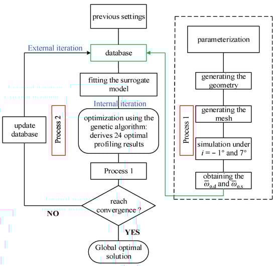
Figure 7.
The framework of the auto-optimization design.
The first step (process 1) is to generate the initial database, as marked by the dashed box in the framework. The variable interval for each of the 102 variables employed in profiling is divided into ten discrete levels. A random combination is then applied for the variables and generates a sampling set of 550 different profiling cases. After meshing and simulating all cases under the design point (i = −1°) and near-stall point (i = +7°), respectively, their overall total pressure loss can be obtained according to
where P* and P represent the total pressure and the static pressure. The subscripts “in” and “out” mean the inlet and outlet of the computational domain. Here, and stand for the total pressure loss at the design and near-stall point. Then, and will be added to the sampling set as the performance parameters.
The second step (process 2) is to conduct the optimization. A bi-objective optimization is employed to design the profiling for the minimum and . The process comprises two layers of iteration. The internal optimization iteration is formed by a radial basis function neural network in place of the CFD solution, and a genetic algorithm (with NSGA-II searching strategy) as the optimizer. Twenty-four individuals along the Pareto front are then selected as the result of the internal iteration. After that, in the outer iteration, CFD simulation is applied for these individuals to calculate their results. The 24 end wall profiling cases are added to the sampling database to refine the neural network and trigger the next external iteration. Although the optimization design should process as many outer iterations as possible before it reaches convergence, considering that the external iteration is rather time-consuming, the maximum external iteration is limited to 30 steps for a compromise.
3. Results and Discussion
3.1. Profiling Results
Figure 8a records the total pressure loss of the baseline case (red star), all the initial samples in the database (blue dots), and all the cases designed in the optimization process (white dots). The vertical and horizontal axes indicate the value of and . The position of the Pareto Front is roughly labeled with red dashes. The value of has been reduced by around 0.15% at most, while is almost up to 3.5%. The shape of the Pareto Front indicates the optimum flow control rules at the design point and the near-stall point are generally independent of each other. Three cases around the Pareto Front (labeled case A, case B, and case C) with an extra profiling case near the top-left of the map (i.e., case D) are selected to investigate the flow control mechanism. Define Δ as the variation of total pressure loss relative to the baseline cascade, i.e.,
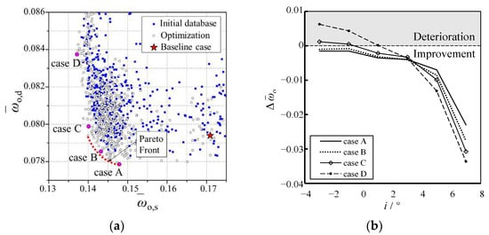
Figure 8.
The total pressure loss of profiling cases. (a) All cases in the optimization design process; (b) the variation of total pressure loss of case A to case D at multiple incidences.
Then Δ of the four selected cases under different incidences can be calculated, as shown in Figure 8b. It is seen that the four cases show a continuous decrease in Δ as i increases but with a changing ranking: the best case for different working conditions is, in turn, case A (i = −3°, −1° and 1°), case B (i = 3°), and case D (i = 5° and 7°). It indicates that although the bi-objective optimization is to minimize and , the selected cases generally find their best-matching incidence between i = −1° and 7°. Besides, all of them improve the performance of the cascade when i > 3°.
Figure 9 shows the profiling of the four selected cases. The right column presents the shape of SS corner profiling on the hub end wall (marked by a red color). A notable regular change from case A to case D is that the maximum thickness (θ) gradually increases, and its axial position (Ca,θ) gradually approaches the LE. Considering increases from case A to D and decreases in the same order, it is reasonable to believe that these regular changes of the combined profiling should be associated with the variation of the most effective flow control rules from the design point to the near-stall point. The left column presents the contour of normalized waviness on the SS (δSS). The significant concave and convex mainly appear near the front half of the SS, but there are no apparent similarities or regular changes. The middle column presents the end wall profiling using the contour of the normalized height of the end wall (δEW). It notably changes in the front-end wall area near the SS (marked by white dots), which gradually “rises” from case A to D.
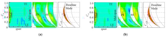
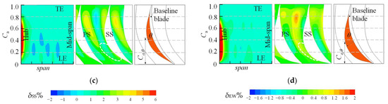
Figure 9.
Profiling results on the end wall, SS, and SS corner. (a) Case A; (b) Case B; (c) Case C; (d) Case D.
Above all, in the order of case A, B, C, and D, the representative cases show a regular change in the maximum thickness and the axial position of the corner profiling and the front suction side area of the end wall. These changes may likely associate with the control of corner separation under multiple working conditions.
3.2. The Coupled Effect of the End Wall Profiling and the SS Profiling
A correlation analysis was first given here to figure out how the end wall profiling and SS profiling would improve the performance of the SS corner profiling. Figure 10 shows the correlation coefficients between profiling parameters and at the design point and near-stall point to find out where the most influential parameters are located. The black bars are the top 15 Spearman correlation coefficients (the Spearman correlation coefficient is a nonparametric measure of statistical dependence of ranking between two variables. A value of +1 means a perfect association of rank and −1 means a perfect negative association between ranks. The closer the value is to 0, the weaker the association between the two ranks). The red bars are partial correlation coefficients (a partial correlation coefficient is a measure of the linear dependence of a pair of random variables from a collection of random variables in the case where the influence of the remaining variables is eliminated. So, if there is a high Spearman correlation coefficient and a low partial correlation coefficient for a pair of variables, it indicates this close relation is dependent on other variables rather than between themselves) between the parameters and total pressure loss coefficient, controlling for all the other profiling parameters. It shows that at both working conditions, the Spearman correlation coefficients of ω1 and γ1 are the only two coefficients that are larger than 0.5. Note that ω1 and γ1 are both for the SS corner profiling, belonging to the sinusoidal function with the period of 2Ca. At the design point, the values of Spearman correlation coefficients are close to the partial correlation coefficients, and all four correlation coefficients are negative. At the near-stall point, the value of the partial correlation coefficient between γ1 and is much lower than the Spearman correlation coefficient, as shown in Figure 10b, and all four correlation coefficients become positive.
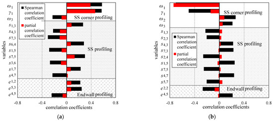
Figure 10.
Correlation analysis between profiling parameters and . (a) i = −1°; (b) i = 7°.
A quantitative analysis is further carried out here, based on the two typical cases for the design point and near-stall point, i.e., case A and case D. The geometries of SS corner profiling, end wall profiling, and SS profiling are drawn from case A and case D. They are then applied separately to the baseline cascade, and labeled with the subscript of C, EW, and SS, respectively. The CFD results of these partial profiling cases are listed in Table 1. For each working condition, the first column shows their overall loss; the second column shows the loss reduction compared to the baseline case; and the third column shows the percentage of the loss reduction relative to case A or case D. So, the values in the third column somewhat represent how these partial profiling cases contribute to the overall effect of the combined profiling cases.

Table 1.
The quantitative analysis of the partial profiling cases.
The results show that the SS corner profiling has the most primary contribution to the reduction of separation loss, for the decrease/increase in and in case AC and DC are most close to (or almost the same as) in case A and case D. The end wall profiling ranks second but is much less critical. Only for the design point does the variation caused by case AEW and case DEW account for more than 10%; however, their absolute effect in reducing can be nearly ignored. The SS profiling in this paper seems to have the minimum influence among all three types of profiling.
Figure 11 provides the plots of cp and confirms that the minor contributions of the end wall profiling and the SS profiling are because of their minor effects on the flow field rather than canceling each other out. Among the plots, those of end wall profiling mainly vary the value of cp below 20%span; those of the SS profiling have the minimum influence, which can hardly be identified. By comparison, the plots of the SS corner profiling show that their impact on cp can be extended even to the mid-span region. This is because the corner separation extends to the mid-span region, and so are the positive/ negative effects of the SS corner profiling.
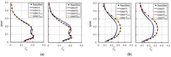
Figure 11.
Pitch-averaged total pressure loss at 0.4Ca downstream of the TE. (a) At the design point (i = −1°); (b) near-stall point (i = 7°).
So far, the first aim of the current study may have a conclusion. The correlation analysis and quantitative analysis both show that in the profiling cases, the effects of end wall profiling and the SS profiling are relatively much lower than the SS corner profiling. So, the above findings insist that using the combined profiling may not improve the compressor’s performance as expected. The corner profiling only takes up a small area. However, it is critical to the control of corner separation and loss.
3.3. Effective Flow Control Rules at Design Point
Based on the previous discussion, case A, B, and D are selected to conclude the effective flow control rules. The design working condition is discussed for the first step. The variation of flow field and loss are given in Figure 12, Figure 13 and Figure 14.
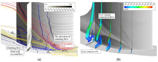
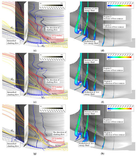
Figure 12.
The flow field and distribution of loss source at the design point. (a) Flow field of the baseline case; (b) loss source of the baseline case; (c) flow field of case A; (d) loss source of case A; (e) flow field of case B; (f) loss source of case B; (g) flow field of case D; (h) loss of case D.
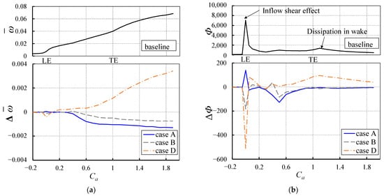
Figure 13.
Development of loss in the passage at the design point. (a) Development of mass-flow-rate-weighted ; (b) development of area-averaged Φ.

Figure 14.
Comparison of pressure field before and after the SS corner profiling. (a) Baseline; (b) case A; (c) case B; (d) case D.
The left column of Figure 12, i.e., Figure 12a,c,e,g, shows the three-dimensional flow field at the design point. The limiting streamlines on the SS and hub surface are presented using thin solid black curves. Critical streamlines are marked out using bold blue curves for a topology analysis. The dashed curves represent the separation line, meaning the position where the boundary layer separates from the solid surface. In contrast, the solid represents the reattachment line, indicating the flow attached to the solid surface. The joint points of the critical streamlines are marked with a solid blue dot for nodes and a blue circle filled white for saddles. It is seen that the limiting streamlines show a complex topology. So, only those matters will be labeled in the figure and discussed in the following discussion.
Figure 12a shows the secondary flow in the baseline case. In the front region of the SS corner, the significant semi-saddle point (S(N)1) and the two brunches of separation lines (sl1 and sl2) mark the starting point and the spreading range of corner separation. Downstream of S(N)1, the cross-passage secondary flow accumulates low-energy fluid in the SS corner, as shown by the limiting streamlines and the contour of secondary kinetic energy (ske). Then, the low-energy fluid climbs to the position of sl3, turns to the reverse direction because of the streamwise pressure gradient, collides to the streamwise boundary layer flow on the SS, and finally separates from sl4. Here, we show the three-dimensional end wall boundary layer flow (yellow streamlines) and the SS boundary layer flow (red streamlines) for a clearer view of this interaction. In Figure 12b, the separation flow from sl4 grows to be a notable “bump-like” blockage with a thin branch stretching to the front part of the end wall, as shown by the transparent grey blockage. The contours show the logarithm of the dissipation function (Φ). Φ is defined as
where μeff includes both the dynamic viscosity and the turbulent viscosity; the meaning of Φ is the rate of kinetic energy that transforms to heat per m3. So, the high value of Φ generally spreads at the border between the blockage and the main flow, which indicates the low-energy fluid induces a strong shear effect between itself and the main flow. Because in the current cascade, Φ means the only factor that increases the entropy of the local airflow, the regions of high Φ are regarded as the loss sources of the whole flow field. Figure 13 shows the distribution of area-averaged Φ and mass-flow-rate-weighted total pressure loss coefficient () along the x-direction. From LE to TE, the loss source in Figure 13b induces the increase in . The two peak values of Φ represent the LE shear effect and the dissipation of the wake. Note that because the blockage of separation flow continuously mixes with the passage flow even in the wave region, the value of thus continuously increases downstream of the TE, and the increment almost reaches the same level as within the passage. Therefore, the main part of the wake loss is still associated with the corner separation.
Compared with the baseline case, case A shows a notable intensified climbing flow around the corner region, as shown by the contours of ske in Figure 12c. This is caused by the variation of a local pressure gradient due to the SS corner profiling. Figure 14 illustrates the iso-curves of the static pressure coefficient (cps) in the corner region. An X-plane is also present to show the variation of the spanwise velocity (Vz). In the boundary layer region, the variation of the climbing flow (Vz) should be affected by the spanwise pressure gradient through
Therefore, as sketched in Figure 14a,b, when the SS corner profiling forms a local convex, the iso-curve of cps becomes dense, showing a higher spanwise pressure gradient pointing to the hub, thus accelerating Vz. As a result, Figure 12c shows that the acceleration of the climbing flow suppresses its reverse trend below sl3 (illustrated using a white arrow). The separation region downstream of sl1 and sl2, including the starting point (S(N)1), thus moves to a more downstream position. The interface between the local three-dimensional end wall boundary layer flow (yellow) and SS boundary layer flow (red) correspondingly moves downstream but with a larger dip angle. The separation line sl4 is also shifted to the TE. All of the above variations of the secondary flow indicate that the corner separation is significantly suppressed. They further bring changes to the shear loss. In Figure 12d, the acceleration of the climbing flow almost eliminates the accumulation of low-energy fluid around S(N)2 on the one hand, and, on the other hand, improves the momentum of fluid at the bottom side of the blockage. The loss source at the border between the low-energy fluid and the main flow thus reduces, as shown by the contours of Φ, in the relative lower region (region 1). Besides, due to the shear effect caused by the three-dimensional boundary layer flow in a higher-span location, the contours of Φ show a slight increase in loss source, labeled as region 2. In Figure 13b, the plot of Φ shows that loss reduction mainly occurs between LE and TE. So, it should be the reduction of loss in region 1 that primarily affects the overall loss reduction.
In case B and case D, the variation of the pressure gradient in the corner region is similar to case A, as shown in Figure 14c,d, but located at a more upstream axial position. Under its influence, the contours of ske in Figure 12e,g show similarly energized climbing flows in cases B and D; thus, both lead to a reduction of loss source in region 1, as shown in Figure 12f,h.
Compared with case A, the value of ΔΦ in case B presents a lower value at LE, a higher value between LE and TE, and almost the same value from TE to the outlet, as shown in Figure 13. The relatively lower value of ΔΦ at the LE has only a little contribution to the variation of Δcp. What makes a difference should be the relative higher ΔΦ from LE to TE, which corresponds to the higher Φ in region 2, as shown in Figure 11f. According to the previous discussion, this negative effect should be relevant to the three-dimensional flow of the inlet end wall boundary layer. Figure 12e shows it collides with the SS boundary layer flow and then turns spanwise at a more upstream position than in case A, with a larger dip angle.
The situation in case D is similar to case B but develops to a further level, as shown in Figure 12g,h. Because of the much higher value of loss source in region 2, the plot of ΔΦ in Figure 13b is even positive from LE to the outlet, meaning that the adverse effects brought by the SS corner profiling in case D overweigh its positive impact from the blade passage to its downstream region. It is clear that even though the SS corner profiling brings a benefit to the control of corner separation by accelerating the climbing flow, it would, on the whole, still deteriorate the corner separation.
The above discussion indicates that the performance of the SS corner profiling is generally decided by the interaction of two different effects on the flow field, which are all summarized in Figure 15.

Figure 15.
Sketched three-dimensional flow at the design point. (a) Baseline; (b) case A; (c) case B; (d) case D.
- The first effect is the acceleration of climbing flow on the SS. As shown by the grey arrows in Figure 15, the acceleration of climbing flow suppresses the reverse trend and energizes the low-energy separation flow. So, it reduces the shear loss and relieves the reverse flow in the separation region in all three profiling cases, regardless of the different maximum thickness and their corresponding streamwise positions.
- The second effect refers to the interaction between the end wall boundary layer and SS boundary layer, as shown by the yellow arrows and red arrows. The previous discussion shows that the relatively high-speed SS boundary layer would collide with the end wall boundary layer and sweep the latter downstream. However, when employing the SS corner profiling, the hump-like solid surface at the bottom of the SS makes it easier for the end wall secondary flow to climb on the SS while blocking the inflow from the LE of SS at the same time. So, the use of SS corner profiling reduces the streamwise momentum of this interaction. As shown in Figure 15, in cases A, B, and D, the more upstream the SS corner profiling is located, the more upstream position it is in for the point where the end wall secondary flow turns to spanwise. As a result, the three-dimensional boundary layer flow induces extra shear loss when it reaches the higher span region. This is an opposing side of the SS corner profiling.
Therefore, the control of corner separation and the overall loss is actually under the trade-off between the positive and negative effects of the SS corner profiling. The positive effect always seems to exist, even for those that finally increase the overall loss. The level of the negative effect is closely associated with its streamwise position and maximum thickness. It can be concluded that a downstream SS corner profiling will always relieve the corner separation by accelerating the local secondary climbing flow. In contrast, the increase in the axial position and maximum thickness of the SS corner profiling would bring more detrimental effects to the control of corner separation, thus making the SS corner profiling less suitable to the design inflow condition. That also explains why it shows the high values of positive Spearman coefficients of γ1 and ω1 shown in Figure 10.
3.4. Effective Flow Control Rules at Near-Stall Point
Figure 16, Figure 17 and Figure 18 compare the flow field and loss between the baseline case and the profiling cases at the near-stall point, with the same definition as Figure 12, Figure 13 and Figure 14. With the previous discussion at the design point in Section 3.3, the following passages will mainly focus on the differences for brevity.
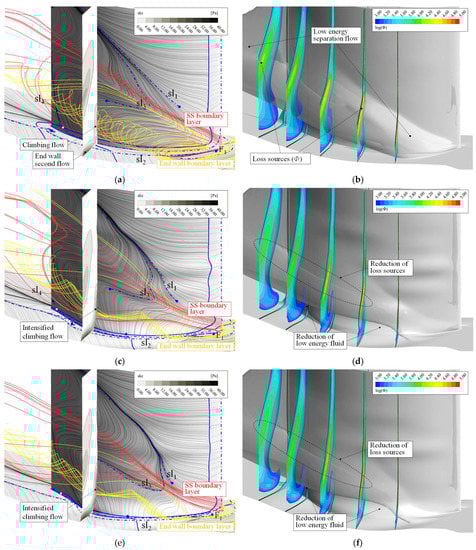
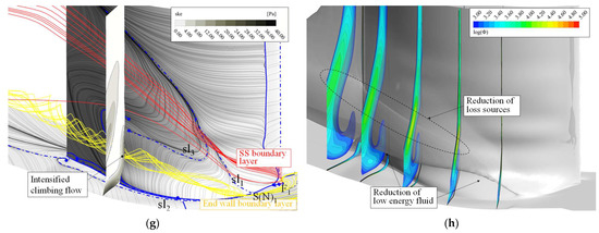
Figure 16.
The flow field and distribution of loss source at the near-stall point. (a) Flow field of the baseline case; (b) loss source of the baseline case; (c) flow field of case A; (d) loss source of case A; (e) flow field of case B; (f) loss source of the case B; (g) flow field of case D; (h) loss of case D.
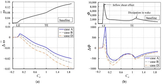
Figure 17.
Development of loss in the passage at the near-stall point. (a) Development of mass-flow-rate-weighted ; (b) development of area-averaged Φ.
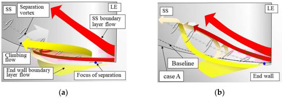
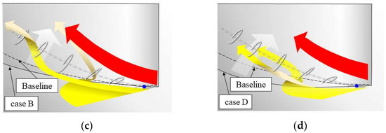
Figure 18.
Sketched three-dimensional flow at the near-stall point. (a) Baseline; (b) case A; (c) case B; (d) case D.
Figure 16a shows the secondary flow in the baseline case. The reverse flow region is significantly enlarged compared to the design point, even extending to the LE. So, the limiting streamlines show no semi-saddle point as in Figure 12a, but instead, a focus (labeled as F1) appears on the end wall of the corner region. The three-dimensional boundary layer flow (yellow streamlines) shows that the separation vortex generates from F1 and occupies the front corner. Some boundary layer flow on the SS (red streamlines) tangles into this vortex and flows downstream. The climbing flow is not as strong as the design point, as shown by the contours of ske. Consequently, the secondary flow shows a strong reverse trend. It accumulates the low-energy fluid in the SS corner region and significantly extends to the passage, finally forming a severe blockage, as shown in Figure 16b. The high value of Φ spreading at the border of the low-energy fluid indicates that the shear loss between the low-energy fluid and the main flow is the primary loss source of the cascade. In Figure 17, the two peak values of the plot of Φ locate at the same position as the design point. The dissipation loss downstream of the TE similarly occupies nearly 50% of the overall loss in the cascade, indicating that the separation loss contributes to the majority part.
According to Figure 16c,d, the positive effect of SS corner profiling in case A is just the same as at the design point. With the increase in the spanwise pressure gradient due to the convex shape of corner profiling, the acceleration of the climbing similarly suppresses its reverse trend and energies the accumulated low-energy fluid (as shown in Figure 16c). So, the separation line sl2 is backward swept, and the shear loss at the border of the low-energy fluid is similarly reduced (as shown in Figure 16d). What makes a difference to the design point is its effect on the three-dimensional boundary layer flow. The end wall boundary layer flow (yellow streamlines in Figure 16c) turns to the spanwise direction as at the design point. However, the SS boundary layer (red streamlines in Figure 16c) directly rushes to the low-energy fluid. The shear loss at the top of the low-energy separation flow is thus not increased as at the design point.
Compared with case A, case B shows a similar variation in its flow field but a more intensified SS boundary layer flow (as shown in Figure 16e). The three-dimensional end wall boundary layer flow is seen as more downstream swept. The contours of Φ in Figure 16f and the plot in Figure 17 show that the SS corner profiling in case B further reduces the shear loss around the LE and downstream of the TE. Case D presents an entirely different topology of limiting streamlines compared to the previously mentioned cases. The reverse trend of the climbing flow at the bottom of the SS is so relieved that the semi-saddle point S(N)1 appears on the corner. The corner separation region is, therefore, significantly rearward shifted. The three-dimensional SS boundary layer flow seems more intensified than in case B. The accumulation of low-energy fluid, including the corresponding shear loss, is reduced in the full range of the passage. The spanwise turning of the end wall boundary layer flow shows no adverse effect on the shear loss in cases B and D.
The above discussion indicates that although the SS corner profiling seems to have a single positive effect on the cascade’s performance, its influence still includes two aspects on the flow field, as shown in Figure 18.
- The first effect is the acceleration of climbing flow on the SS, as shown by the grey arrows in Figure 18. The details are not repeated because it is the same as the design point.
- The second effect is the interaction between the end wall boundary layer and the SS boundary layer, as shown by the yellow arrows and red arrows. The previous discussion at the design point shows that employing the SS corner profiling is more convenient to the end wall secondary flow to climb on the SS, but blocks the relatively high-speed inflow from the LE of SS. However, near the stall point, the high incidence makes the bump-like SS corner profiling more suitable for the inflow. As a result, the SS boundary layer is less likely to be separated near the bottom region of the SS. The more upstream the convex profiling is located, the higher the streamwise momentum for the SS boundary layer flow. As a result, the corner separation will be more effectively reduced, thus leading to a further reduction for overall loss.
Because both effects are favorable to the control of corner separation, it is hard to know which one contributes more to the overall improvement. However, the reduction of overall loss ranks in the turn of case D, case B, and case A, and the thickness of corner profiling increases according to the same order. The correlation analysis in Figure 10b found ω1 is the only parameter whose Spearmen correlation coefficients and partial correlation exceed −0.5. It can be thus deduced that a large thickness of the SS corner profiling should be closely relative to the control of corner separation and the reduction of loss near the stall point.
Besides, considering the effect of the SS corner profiling on the SS boundary layer refers to the development of SS boundary layer flow, which makes case A the best for the design point and case D for the near-stall point, respectively. It can be deduced that each SS corner profiling with a different maximum thickness should have its own optimum inflow condition when the shape of SS corner profiling matches the inflow incidence. That also explains why case B has the lowest loss among all profiling cases when i = 3°.
3.5. Summary of the Effective Flow Control Rules
From the above analysis, the second aim of the paper can have an answer. The most effective flow control rules for the compressor cascade at the different flow conditions can be summarized as follows.
At the design point where the corner separation stays in the rear part of the passage, the most suitable means to suppress the corner separation is to apply a fillet-like SS corner profiling in the mid-chord to the rear part of the passage. The critical flow control mechanism is to accelerate the local climbing secondary flow. As a result, the reverse trend of the climbing flow will significantly reduce, and the low energy fluid due to the corner separation will be energized. The corner separation will thus be downstream shifted and finally reduce the corresponding loss. One needs to pay attention so that the corner profiling must not be designed with a large thickness and upstream position. Otherwise, the corner profiling will negatively affect the inflow boundary layer on the SS and intensify the corner separation, finally increasing the overall loss of the compressor cascade.
At the near-stall point, where the corner separation spreads to a much more extensive range than at the design point, the most suitable means to suppress the corner separation and reduce separation loss is to employ a fillet-like SS corner profiling with a large profiling thickness. The profiling will accelerate the climbing flow on the bottom of the SS with a similar mechanism to the design point. What makes a difference is that the SS corner profiling brings no negative effect but an extra benefit to the interaction between the SS boundary layer and the end wall boundary layer. A larger profiling thickness is found to increase this benefit and help to relieve the corner separation, finally further reducing the overall separation loss.
In addition, the similarities and differences of flow control rules between the design and near stall point indicate a trade-off between the optimum design for the two working conditions. The result shows that a medium value between the design and near-stall well-fitting parameters will make the suction side corner profiling a best-matching case for a medium inflow condition between −1° and +7°, with adequate performance for multiple working conditions.
4. Conclusions
To suppress the corner separation and reduce the corresponding loss, the investigation in this paper proposed a new parametric SS corner profiling method that applies the weighted superposition of sinusoidal functions. A bi-objective auto-optimization design process for the SS corner profiling was then carried out on a high-load linear compressor cascade, with the companion of the end wall profiling and SS profiling. The aim was to investigate the effective flow control rules for the corner separation and then conclude the design rules of the corner profiling under multiple working conditions. The conclusions of the paper are as follows:
- (1)
- Compared to the previously proposed corner profiling method that applies a fixed algorithm with a single-hump of thickness over streamwise, the new approach is more applicable for both application and investigation, for it designs the SS corner profiling with only six variables but enables more flexible shape variation. The simulation result verified the effectiveness of this new method.
- (2)
- The SS corner profiling takes up a small area at both the design and near-stall points. Still, it contributes a more dominant part to suppressing the corner separation and reducing loss than SS and end wall profiling. Using the combined profiling may not improve the performance of the SS corner profiling in compressors as much as expected.
- (3)
- Improving the performance of the cascade at the design point requires the SS corner profiling to be placed in the mid-chord to rear part of the passage, with a limited maximum thickness. The convex shape of the corner profiling would accelerate the climbing secondary flow at the bottom of the SS, suppress its reverse trend, and energize the low-energy separation flow without inducing a strong negative effect to the interaction between the inlet end wall boundary layer and the SS boundary layer flow. In comparison, improving the performance of the cascade at the near-stall point requires the SS corner profiling to be placed with a large maximum thickness. This is so that the corner profiling would induce a positive acceleration of the climbing secondary flow similar to the design point while benefitting the interaction between the inlet end wall boundary layer and the SS boundary layer flow. In both working conditions, the improvement of the overall performance depends on the relief of the corner separation.
- (4)
- The similarities and differences of flow control rules between the design and the near-stall point indicate a trade-off between the optimum design for the two working conditions. A medium value between the design and near-stall well-fitting parameters will make the suction side corner profiling a best-matching case for a medium inflow condition with adequate performance for multiple working conditions.
Author Contributions
Conceptualization, X.L.; methodology, J.D.; software, J.D.; validation, X.L., H.C. and H.L.; formal analysis, J.D.; investigation, X.L.; resources, X.L.; data curation, J.D.; writing—original draft preparation, J.D.; writing—review and editing, J.D. and X.L.; visualization, X.L.; supervision, X.L. and H.L.; project administration, X.L.; funding acquisition, X.L. and H.L. All authors have read and agreed to the published version of the manuscript.
Funding
The work is funded by the National Natural Science Foundation of China (Grant No. 51906027, 52176036 and 52076179), Doctoral Initiation Research Funds of Liaoning province (Grant No. 2019-BS-027), and the Fundamental Research Funds for the Central Universities (Grant No. 3132022112).
Conflicts of Interest
The authors declare that they have no known competing financial interest or personal relationships that could have appeared to influence the work reported in this paper.
References
- Lakshminarayana, B.; Horlock, J.H. Leakage and Secondary Flows in Compressor Cascades; British ARC, R&M: London, UK, 1967; Volume 3483, pp. 1–60. [Google Scholar]
- Lei, V.M.; Spakovszky, Z.S.; Greitzer, E.M. A criterion for axial compressor hubcorner stall. J. Turbomach. 2008, 130, 031006. [Google Scholar] [CrossRef] [Green Version]
- Zhang, Y.F.; Mahallati, A.; Benner, M. Experimental and numerical investigation of corner stall in a highly-loaded compressor cascade. In Proceedings of the ASME Turbo Expo, Düsseldorf, Germany, 16–20 June 2014. GT2014-27204. [Google Scholar]
- Ma, W.; Ottavy, X.; Lu, L.P.; Leboeuf, F.; Gao, F. Experimental study of corner stall in a linear compressor cascade. Chin. J. Aeronaut. 2011, 24, 235–242. [Google Scholar] [CrossRef]
- Li, X.J.; Chu, W.L.; Wu, Y.H. Numerical investigation of inlet boundary layer skew in axial-flow compressor cascade and the corresponding non-axisymmetric end wall profiling. Proc. Inst. Mech. Eng. A J. Power Energy 2014, 228, 638–656. [Google Scholar] [CrossRef]
- Gbadebo, S.A.; Cumpsty, N.A.; Hynes, T.P. Three-dimensional separations in axial compressors. J. Turbomach. 2005, 127, 331–339. [Google Scholar] [CrossRef]
- Lewin, E.; Kožulović, D.; Stark, U. Experimental and Numerical Analysis of Hub-Corner Stall in Compressor Cascade. In Proceedings of the ASME Turbo Expo, Glasgow, UK, 14–18 June 2010. GT2010-22704. [Google Scholar]
- Zambonini, G.; Ottavy, X.; Jochen, K. Corner separation dynamics in a linear compressor cascade. J. Fluid Eng. 2017, 139, 061101. [Google Scholar] [CrossRef]
- Burguburu, S.; Pape, A. Improved aerodynamic design of Turbomachinery bladings by numerical optimization. Aerosp. Sci. Technol. 2003, 7, 277–287. [Google Scholar] [CrossRef]
- Ma, S.; Chu, W.; Zhang, H.; Li, X.; Kuang, H. A combined application of micro-vortex generator and boundary layer suction in a high-load compressor cascade. Chin. J. Aeronaut. 2019, 32, 1171–1183. [Google Scholar] [CrossRef]
- Leroy, H.S.; Yeh, H. Sweep and dihedral effect in axial flow turbomachinery. J. Basic Eng. 1963, 85, 401–413. [Google Scholar]
- Breugelmans, F.A.H.; Carels, Y.; Demuth, M. Influence of Dihedral on the Secondary Flow in a Two-Dimensional Compressor Cascade. In Proceedings of the Tokyo International Gas Turbine Congress, Tokyo, Japan, 24–28 October 1983. 83-GTJ-12. [Google Scholar]
- Sasaki, T.; Breugelmans, F. Comparison of sweep and dihedral effects on compressor cascade performance. J. Turbomach. 1998, 120, 454–463. [Google Scholar] [CrossRef]
- Roy, B.; Laxmiprasanna, P.A.; Borikar, V.; Batra, A. Low Speed Studies of Sweep and Dihedral Effects on Compressor Cascades. In Proceedings of the ASME Turbo Expo, Amsterdam, The Netherlands, 3–6 June 2002. GT2002-30441. [Google Scholar]
- Denton, J.D. The effects of lean and sweep on transonic fan performance: A computational study. Task Q. 2001, 6, 7–23. [Google Scholar]
- Denton, J.D.; Xu, L. The effects of lean and sweep on transonic fan performance. In Proceedings of the ASME Turbo Expo, Amsterdam, The Netherlands, 3–6 June 2002. GT2002-30327. [Google Scholar]
- Gallimore, S.J.; Bolger, J.J.; Cumpsty, N.A.; Taylor, M.J.; Wright, P.I.; Place, J.M. The use of sweep and dihedral in multistage axial flow compressor blading—Part i: University research and methods development. J. Turbomach. 2002, 124, 521–532. [Google Scholar] [CrossRef]
- Taylor, J.V.; Miller, R.J. Competing three-dimensional mechanisms in compressor flows. J. Turbomach. 2017, 139, 021009. [Google Scholar] [CrossRef]
- Ji, L.; Shao, W.; Yi, W.; Chen, J. A model for describing the influences of SUC-EW dihedral angle on corner separation. In Proceedings of the ASME Turbo Expo, Montreal, QC, Canada, 14–17 May 2007. GT2007-27618. [Google Scholar]
- Ji, L.; Tian, Y.; Li, W.; Yi, W.; Wen, Q. Numerical studies on improving performance of rotor-67 by blended blade and endwall technique. In Proceedings of the ASME Turbo Expo, Copenhagen, Denmark, 11–15 June 2012. GT2012-68535. [Google Scholar]
- Li, J.; Ji, L.; Yi, W. Experimental and numerical investigation on the aerodynamic performance of a compressor cascade using blended blade and end Wall. In Proceedings of the ASME Turbo Expo, Charlotte, NC, USA, 26–30 June 2017. GT2017-63879. [Google Scholar]
- Li, J.; Ji, L.; Yi, W. The use of blended blade and end wall in compressor cascade: Optimization design and flow mechanism. In Proceedings of the ASME Turbo Expo, Oslo, Norway, 11–15 June 2018. GT2018-76048. [Google Scholar]
- Reutter, O.; Hemmert-Pottmann, S.; Hergt, A.; Nicke, E. Endwall contouring and fillet design for reducing losses and homogenizing the outflow of a compressor cascade. In Proceedings of the ASME Turbo Expo, Düsseldorf, Germany, 16–20 June 2017. GT2014-25277. [Google Scholar]
- Meng, T.; Yang, G.; Zhou, L.; Ji, L. Full blended blade and endwall design of a compressor cascade. Chin. J. Aeronaut 2021, 34, 79–93. [Google Scholar] [CrossRef]
- Reising, S.; Schiffer, H. Non-axisymmetric end wall profiling in transonic compressors.Part I: Improving the static pressure recovery at off-design conditions by sequential hub and shroud end wall profiling. In Proceedings of the ASME Turbo Expo, Orlando, FL, USA, 8–12 June 2009. GT2009-59133. [Google Scholar]
- Reising, S.; Schiffer, H. Non-axisymmetric end wall profiling in transonic compressors. Part II: Design study of a transonic compressor rotor using nonaxisymmetric end walls optimization strategies and performance. In Proceedings of the ASME Turbo Expo, Orlando, FL, USA, 8–12 June 2009. [Google Scholar]
- Li, X.; Chu, W.; Wu, Y.; Zhang, H.; Spence, S. Effective end wall profiling rules for a highly loaded compressor cascade. Proc. Inst. Mech. Eng. A J. Power Energy 2016, 230, 535–553. [Google Scholar] [CrossRef] [Green Version]
- Varpe, M.K.; Pradeep, A.M. Benefits of nonaxisymmetric endwall contouring in a compressor cascade with a tip clearance. J. Fluids Eng. 2015, 137, 051101. [Google Scholar] [CrossRef]
- Winter, K.; Hartmann, J.; Jeschke, P.; Lahmer, M. Experimental and numerical investigation of streamwise surface waviness on axial compressor blades. In Proceedings of the ASME Turbo Expo, San Antonio, TX, USA, 3–7 June 2013. GT2013-95983. [Google Scholar]
- Cheng, J.; Chen, J.; Xiang, H. A surface parametric control and global optimization method for axial flow compressor blades. Chin. J. Aeronaut 2019, 32, 1618–1634. [Google Scholar] [CrossRef]
- Wang, B.; Wu, Y.; Liu, K. Numerical investigation of passive flow control using wavy blades in a highly-loaded compressor cascade. In Proceedings of the ASME Turbo Expo, Oslo, Norway, 11–15 June 2018. GT2018-76147. [Google Scholar]
- Li, X.; Chu, W.; Zhang, H. Investigation on Relation between Secondary Flow and Loss on a High Loaded Axial-Flow Compressor Cascade. J. Propuls. Technol. 2014, 35, 914–925. [Google Scholar]
Publisher’s Note: MDPI stays neutral with regard to jurisdictional claims in published maps and institutional affiliations. |
© 2022 by the authors. Licensee MDPI, Basel, Switzerland. This article is an open access article distributed under the terms and conditions of the Creative Commons Attribution (CC BY) license (https://creativecommons.org/licenses/by/4.0/).