2D Numerical Study on the Flow Mechanisms of Boundary Layer Ingestion through Power-Based Analysis

Abstract

This paper aims to establish an approach of power bookkeeping in a numerical study. To study the process of power conversion coursed in the flow field, the methodology employs a power-based analysis to quantify power terms. This approach is examined in a simulation of jet flow and then applied to the cases of an isolated actuator disc and an isolated flat plate. Eventually, a numerical simulation is carried out for the boundary layer ingestion (BLI) case that integrates the flat plate and a wake-filling actuator disc. This study quantitatively discusses the mechanisms of BLI under the conditions of laminar and turbulent flow. The proposed power-based analysis might offer insights for the aircraft aerodynamic design using favorable airframe propulsion integration.

1. Introduction

Boundary layer ingestion (BLI) has been investigated as a novel configuration for aircraft by integrating airframe and propulsion systems to reduce fuel consumption and emissions. For example, the Boeing blended wing body aircraft, which merges its fuselage with the wing, adopts a BLI configuration. The research on this aircraft indicates a 10% reduction in fuel burn due to BLI [1]. BLI was also chosen for the “Silent Aircraft” concept which aims to reduce noise emission. The study of this aircraft shows that the fuel consumption can be reduced by 3~4% due to BLI [2]. BLI is also used in the NASA Hybrid Wing Body N3-X aircraft. The research carried on the aircraft configuration estimated that BLI could bring in a 7% reduction in the required power [3]. The D8 aircraft, whose fuselage is characterized by a double bubble cross-section also uses BLI to increase the total efficiency. Numerical and experimental assessments claim that BLI could lead to a 6~9% reduction in power consumption [4,5,6].

In these recent studies on BLI, the analysis of aircraft performance has employed multiple methods. Conventional approaches access aerodynamic force (momentum) to evaluate aircraft performance [7], such as thrust/drag bookkeeping and drag breakdown. Nevertheless, these approaches have difficulties to study aircraft performance in BLI configuration, because drag and thrust are ambiguously defined when airframe and propulsion systems are tightly integrated. To deal with this issue, methods based on power have been introduced. Drela [8] proposed a power balance method to evaluate mechanical power in the flow field. This method has been employed in the D8 aircraft project [4,5,6]. Arntz, Atinault [9] improved this method by taking thermal power into account. The improved method is called exergy-based method which has been used to study BWB aircraft [10] and turbomachines of aero engines [11]. These methods based on mechanical power or exergy are considered power-based methods which are capable of evaluating the actual aircraft power consumption without ambiguity. This is critical to study the actual BLI benefit: The saving of power consumption is attributed to the reduction of the viscous dissipation of the aircraft wake and the propulsive jet [8]. Moreover, power-based analysis is particularly important in addressing controversial issues such as “BLI efficiency paradox”: The observation of power coefficients being greater than one is mainly associated with the power pertaining to ingested wake (boundary layer), which is an input power for the BLI propulsor [12], and a transient power for the entire aircraft [13].

It is noted that the original power-based methods are established within a well-defined control volume. This simple control volume limits the capability of studying the evolution process of an individual power term; therefore, it is not possible to know the details of how aircraft components influence the power conversion process. This incapability motivates the current study to propose a segregated computational domain to trace the change of power terms, thereby illustrating the detailed power conversion process. On the other side, previous studies using power-based analysis reported different values of power saving due to BLI, ranging from 3% to 30% [2,14]. Indeed, one could argue that the benefit due to BLI depends on aircraft geometry and flow conditions. However, it is necessary to study the flow mechanisms of BLI in order to quantify how much improvement in aircraft performance can be expected for aircraft design in the most optimistic scenario. This motivates a quantitative study to evaluate the impacts of an individual mechanism on the overall performance.

Building upon the above-mentioned research line, this study aims to quantitatively analyze the power conversion process of BLI by employing numerical simulations. An approach of power bookkeeping is established to investigate the power conversions related to BLI. This power-based analysis with a segregated computational domain is performed to post-process the simulation data such that the detailed processes involved in the power conversion can be determined. This paper has two main objectives: The first one is establishing the detailed process of the typical power conversions for typical models, namely, an isolated actuator disc, an isolated flat plate, and a vehicle which combines the actuator and the flat plate in a BLI configuration; these typical power conversions are closely related to the mechanisms of BLI. The second objective is quantifying the various influences and analysing the mechanisms of BLI.

To achieve these two major objectives, power-based analysis in this paper is restricted only to the mechanical powers which exclude the thermal power in numerical simulations. Additionally, numerical simulations are limited to 2D (planar) steady (laminar and turbulent) incompressible flows, which allows the exclusion of complicated flow physics, such as compressibility, heat transfer, etc. These simplifications allow the analysis to be focused on the main mechanisms of BLI. To establish a progressive understanding, this paper is organized as follows: Section 2 introduces the principle of combining power-based analysis with numerical simulations, and then demonstrates the power bookkeeping of a simple laminar jet. In Section 3, the power-based analysis is applied to the simulations of laminar flows. This section analyses the typical power conversion processes of an actuator disc, a flat plate and a BLI-integrated vehicle in laminar flows. These cases enable the discussion about the flow mechanisms of BLI. Section 4 mainly studies BLI-related power conversions in turbulent flows, and simulations of the flat plate and the integrated vehicle in turbulent flows are discussed. The main conclusions of this research are summarized in Section 5.

2. Power-Based Analysis in Computation Fluid Dynamics

Power-based analysis evaluates the “powers” of the flow. It utilizes the integral form of the mechanical energy equation which is obtained by multiplying the momentum equation with velocity vector [8]. Numerical simulation using Computation Fluid Dynamics (CFD) resolves Navier–Stokes equations within the computational domain, obtaining the flow field with fine details. To establish a progressive understanding, this section elaborates why power-based analysis is capable of processing the flow field obtained from numerical simulations, then the requirements of the computational domain for the analysis are discussed. Finally, this section demonstrates the power-based analysis of a simple laminar jet.

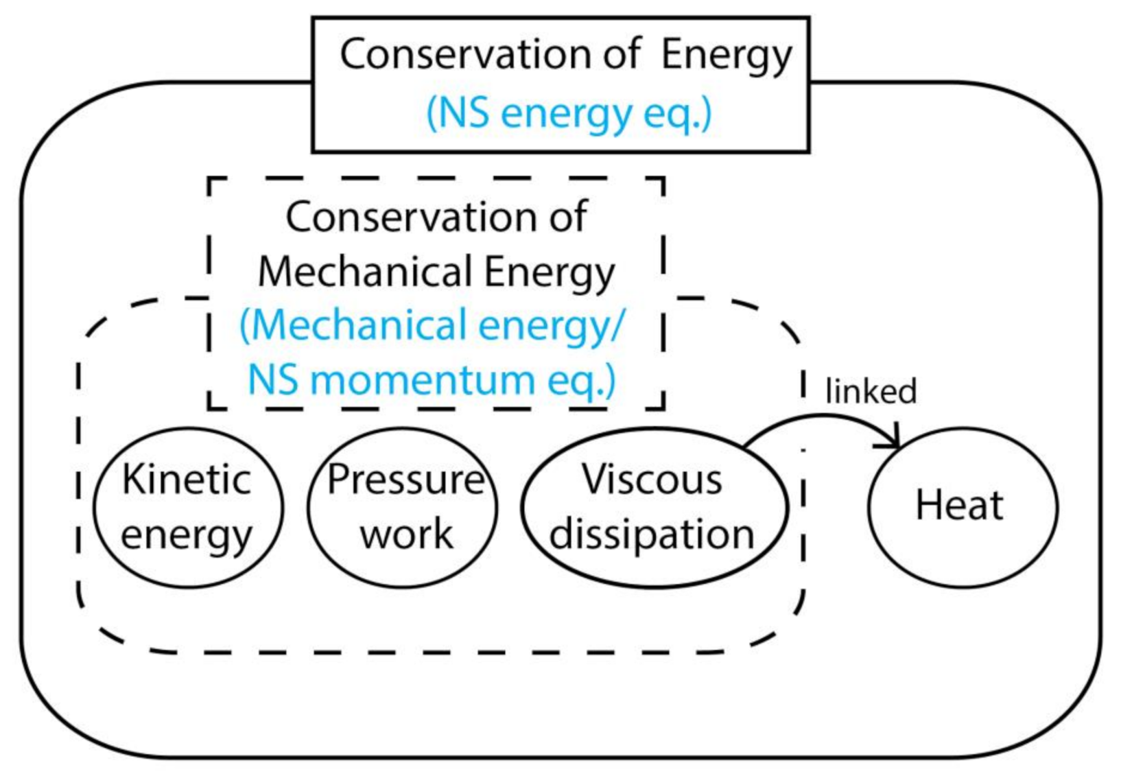
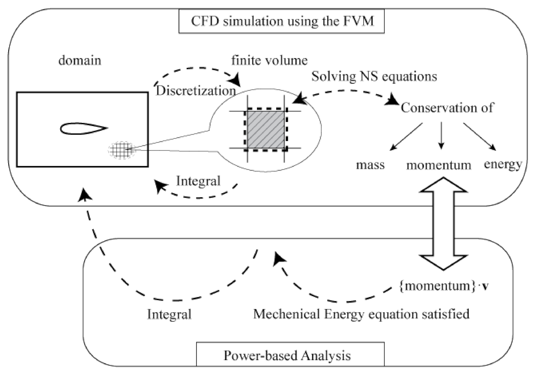
2.1. Compatibility between Finite Volume Method and Power-Based Analysis

Depending on the numerical method of solving partial differential equations, CFD can be categorized as finite volume, finite difference, or finite element method [15]. Despite the choice of the method, conservation laws must be satisfied in CFD simulations. For incompressible viscous flow, the equations of continuity, momentum, and energy are expressed as Equations (1)–(3). Enthalpy h is obtained through the thermodynamic equation of state, as in Equation (4) [16]. Constant values are given to the air properties of density ρ, (laminar) viscosity μ_lam, thermal conductivity k, and specific heat C_p. Due to the constant air properties, it is possible to solve the continuity and momentum equations for the velocity and the pressure, without regard for the energy equation or the temperature [17]. In incompressible flow, viscous dissipation Φ expressed by Equation (5) is not able to generate enough heat to cause large temperature changes. Nevertheless, it is a vital power-loss term in the proposed power-based analysis. The simulation of the turbulence viscous flow is enabled by the Boussinesq hypothesis. Governing equations are coupled with a turbulence model through the decomposition of viscosity μ given in Equation (6), where turbulent viscous μ_tur is determined by the turbulence model.

$$\nabla ·V=0$$

(1)

$$\rho \frac{DV}{Dt}=-\nabla p+\mu {\nabla }^{2}V$$

(2)

$$\rho \frac{Dh}{Dt}=\frac{Dp}{Dt}+\mathrm{div}\left(k\nabla T\right) + \Phi$$

(3)

$$h=C_{P}T$$

(4)

$$\Phi =\mu \left[2{\left(\frac{\partial u}{\partial x}\right)}^2+2{\left(\frac{\partial v}{\partial y}\right)}^2+{\left(\frac{\partial v}{\partial x}+\frac{\partial u}{\partial y}\right)}^2\right]$$

(5)

$$\mu ={\mu }_{lam}+{\mu }_{tur}$$

(6)

In fluid mechanics, the mechanical energy equation is different from the energy equation [18]. The former is obtained by multiplying the momentum equation (vector form) with velocity (vector form), whereas the latter is about the first law of thermodynamics. Viscous dissipation bridges the two equations: Mechanical power is transferred into heat via viscous dissipation, causing the temperature change in the flow field. The diagram in Figure 1 depicts the relation between the conservations of energy (Navier–Stokes energy equation) and mechanical energy (mechanical energy/Navier–Stokes momentum equation). On the other side, power-based analysis uses an integral form of the mechanical energy equation [8,18]. In principle, power-based analysis should comply with simulations when conservation laws are satisfied. This paper limits the power-based analysis to study mechanical power because thermal energy is deemed as less relevant in the discussion of the conversion of mechanical energy and this simplification enables discussions emphasising the physical mechanism involved in BLI.

The top drawing of Figure 2 illustrates the simplified flowchart of the CFD simulation that solves the Navier–Stokes equations by utilizing the Finite Volume Method (FVM). For the simulation, an entire computational domain is discretized into a large number of finite control volumes. The FVM computes flow variables of an individual volume such that the conservation of mass, momentum, and energy are satisfied. Meanwhile, the flux of the conserved quantities is transferred to the adjacent volumes so that conservation laws can be satisfied within the entire domain. On the other side, power-based analysis applies the integral form of the mechanical energy equation, a variant of the momentum equation. As a result, mechanical energy conservation should be satisfied within the entire computational domain. This relation between power-based analysis and FVM is schematically shown in Figure 2. The above discussion implies that power-based analysis complies with the numerical simulation using FVM, which is available in commercial CFD software.

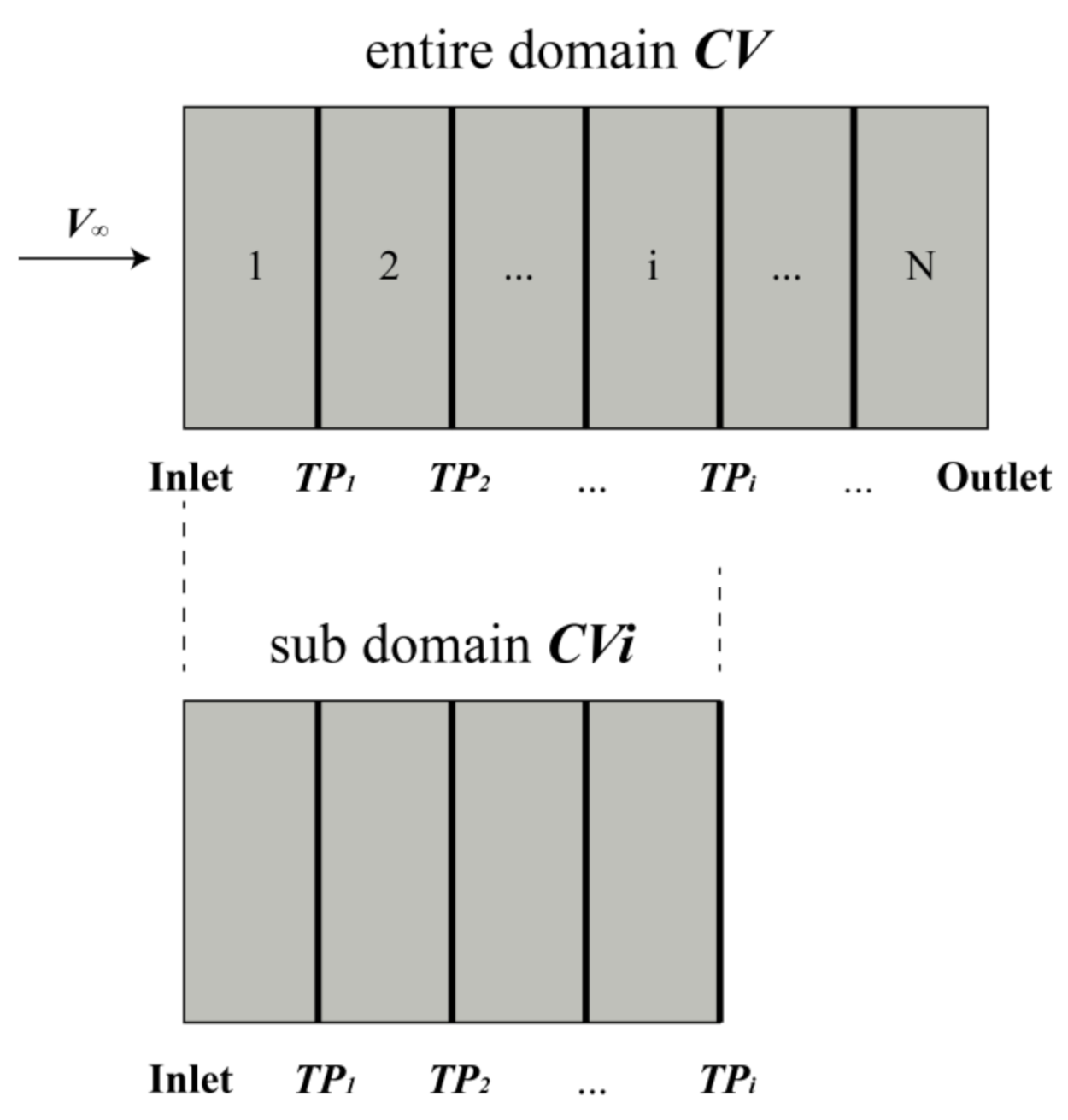
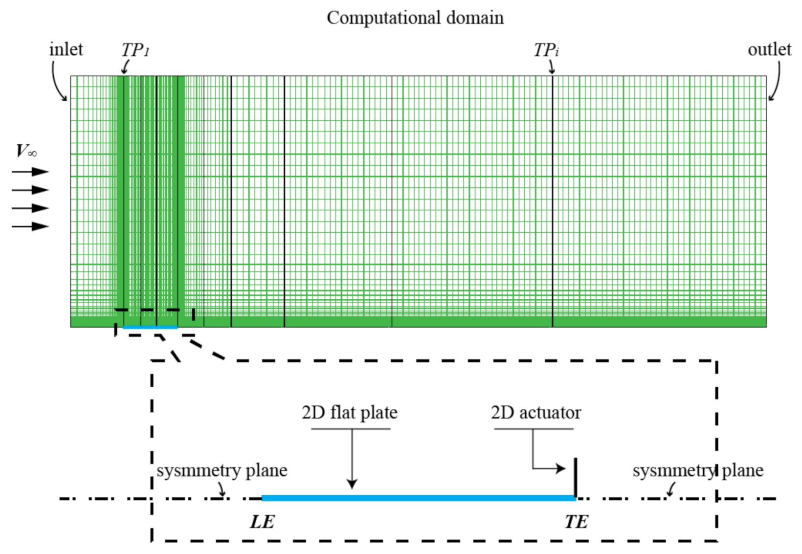
2.2. Computational Domain

Power-based analysis is capable of showing power terms at corresponding Trefftz Planes (TP), such that the change in power can be tracked and power conversion can be analyzed. For this purpose, a special computational domain in CFD simulations is required, as introduced in the following paragraphs.

For a 2D computational domain with the horizontal free stream velocity vector V_∞, a TP is defined as a vertical plane to assess the power of energy deposition rates, such as wake kinetic energy flow $\dot{K{E}_w}$ and pressure work-defect rate Ė_p. Series of vertical TPs are placed along the x-axis to illustrate the change of energy deposition rates. These TPs separate the entire domain into individual Control Volumes (CV), as shown at the top of Figure 3. For a certain TP denoted by the TP_i, a corresponding subdomain CV_i is defined as the collection of individual domains from the first individual CV to the one just upstream TP_i. This subdomain is used to evaluate the power in the form of volume integral, such as viscous dissipation rate Φ. Power-based analysis assesses Φ at different x locations and thus traces the change of this power. It is noted that the unit of mechanical power term is [W], by using SI units for all flow variables.

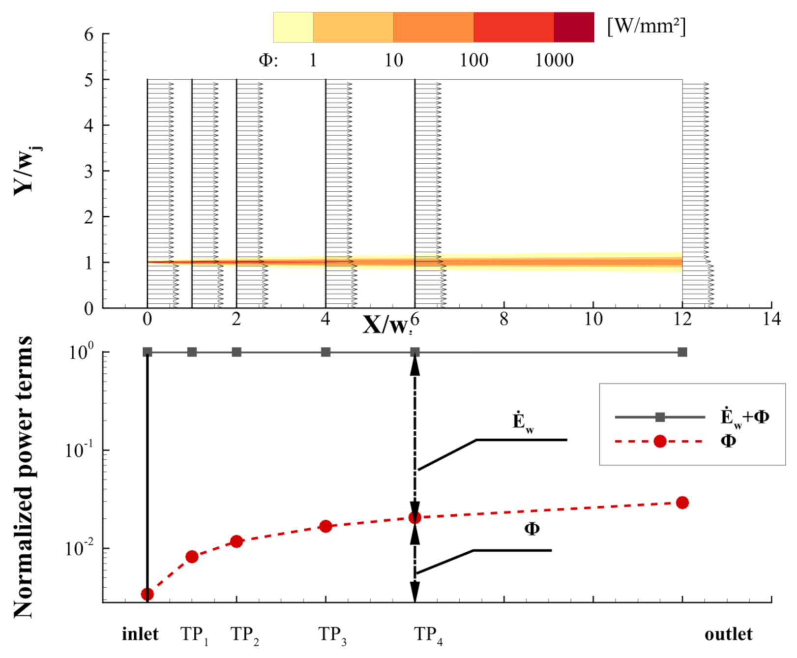
2.3. Power Bookkeeping of Laminar Jet

Axial jet and wake are the elementary flows to study the mechanisms of BLI [13]. The jet is defined as the flow axial velocity larger than V_∞, and wake is characterized by the axial velocity lower than V_∞. This part discusses the power conversion of an axial jet. The flow field is obtained from 2D steady laminar incompressible Navier–Stokes CFD simulations. Additionally, the simulation results are post processed through power bookkeeping.

In this case, a simple jet is defined by the axial velocity u_j of 12 m/s, higher than the V_∞ of 10 m/s, and the pressure at the inlet is ambient pressure p_∞. The Reynolds number based on the jet height is about 1400, indicating that the flow is laminar. The air is set to have a density ρ of 1.225 kg/m³ and a viscosity μ_lam of 1.7894 × 10⁻⁵ Ns/m². Specific heat C_P is 1006.43 J/(kgK) and thermal conductivity k is 0.0242 W/(mK). The jet enters a 5w_j × 12w_j rectangular domain, as shown in Figure 4 (top). This domain is bounded by a vertical inlet, a vertical outlet, and two horizontal planes (top and bottom planes). The bottom plane is defined as a symmetric boundary for this symmetrical flow model. The top plane is also set as a symmetry plane to prevent flow penetration. There are four TPs inside the domain as interior planes, as shown in Figure 4 (bottom). These TPs separate the domain into individual volumes that combine into subdomains.

The simulation employs the commercial software FLUENT, using a structural mesh with 4680 cells.

Table 1. Mesh sensitive study for the simulation of jet.

Cell Number	Φ (Watt)	Relative Difference
4680	0.008521953	0.9%
18,720	0.008533576	0.8%
74,880	0.008569048	0.4%
299,520	0.008603587	0.0%

presents the mesh sensitive study, showing relative differences of the total viscous dissipation Φ with regard to the value of the finest mesh which contains 0.3 million cells. The chosen mesh size keeps simulation results grid independent. The mesh is refined near the shear layer region, as shown at the bottom of Figure 4. The simulation uses the second-order upwind for spatial discretization and the SIMPLE scheme for the pressure-velocity coupling [20,21].

Power-based analysis assesses mechanical power to process the simulation results of the flow field. Ė_w and Φ are the involved power terms for the elementary flows [13]. Ė_w denotes the energy flow rate crossing a trefftz plane, consisting of kinetic energy flow rate KĖ_w,i and pressure work rate Ė_p,i as in Equation (7). Kinetic energy flow rate can be further broken down into axial component Ė_a and transversal component Ė_v, as given in Equation (8). It is noted that the kinetic energy component is based on the relative velocity (with regard to V_∞), hence KĖ_w,i is positive for both jet and wake flows. Pressure power Ė_p is expressed in Equation (9), denoting the pressure work which could be potentially transferred into kinetic energy. Φ stands for the viscous dissipation in a subdomain CV (corresponding to the trefftz plane), as given in Equation (10). In the flow field where velocity gradient exists, the integrant of Φ should be non-zero and positive. Viscous dissipation includes the laminar and turbulent components, whereas the latter component can be removed in this case of laminar jet flow. The two mechanical power terms Ė_w, and Φ establish a power balance equation, as in Equation (11). For an arbitrary trefftz plane TP_i, the summation of the two terms should be constant. As a total power, the summed power for the arbitrary TP_i should be equal to the total power Ė_w,inlet assessed at the inlet.

$$\dot{K{E}_w}+{\dot{E}}_p={\dot{E}}_w$$

(7)

$$\dot{K{E}_w}={\dot{E}}_a+{\dot{E}}_v=\underset{SP}{\overset{}{{\displaystyle \iint }}}\rho u\frac{1}{2}{\left(u-V_{\infty }\right)}^{2}dS+\underset{SP}{\overset{}{{\displaystyle \iint }}}\rho u\frac{1}{2}{v}^{2}dS$$

(8)

$${\dot{E}}_p={{\displaystyle \iint }}_{SP}^{}\left(p-p_{\infty }\right)\left(u-V_{\infty }\right)dS$$

(9)

$$\Phi \cong \underset{CV}{\overset{}{{\displaystyle \iiint }}}{\mu }_{lam}{\left(\frac{\partial u}{\partial y}\right)}^{2}dV$$

(10)

$${\dot{E}}_{w,i}+{\Phi }_i={\dot{E}}_{w,inlet}=const$$

(11)

Table 2. Power terms at various locations of TPs in the simulation of a jet.

Plane	x/wj	Ėw,i/Ėw,inlet	Φi/Ėw,inlet	(Ėw,i + Φi)/Ėw,inlet	(Ėw,i + Φi − Ėw,inlet)/Ėw,inlet
Inlet	0	100.00%	0.00%	100.00%	0.00%
TP1	1	99.05%	0.82%	99.86%	−0.14%
TP2	2	98.67%	1.17%	99.83%	−0.16%
TP3	4	98.13%	1.67%	99.80%	−0.20%
TP3	4	98.13%	1.67%	99.80%	−0.20%
outlet	12	96.84%	2.92%	99.73%	−0.26%

presents the involved power terms accessed at various x locations of the computational domain. Ė_w,i and Φ_i are calculated by using Equations (7)–(10). All the power terms are normalized with the reference value of energy flow rate at the inlet Ė_w,inlet. It is noted that Ė_p,i has a value of zero, because of the constant pressure p_∞ in the entire flow field. As a result, Ė_w,i is equal to KĖ_w,i. The summations of Ė_w,i and Φ_i along the x axis tend to keep constant.

Power bookkeeping of the jet is illustrated by the change of power in Figure 5. The top picture shows the contours of the integrand of Φ. The high-intensity region corresponds to the viscous shear layer. This picture also plots velocity profiles, showing that the profiles tend to be flattened when the jet flows downstream. The bottom figure visualizes the power bookkeeping. The x-axis denotes the x location of TPs, and y-axis corresponds to the power terms tabulated in Table 2. This figure illustrates the power conversion process of the jet: Dissipation Φ (red dashed line) irreversibly increases along with the x-axis, whereas Ė_w,i (the gap between the two power lines) gradually reduces. The summation of Ė_w,i and Φ is almost constant as total power. At the outlet, 2.92% of the total power is converted into dissipation Φ.

A tiny reduction of the total power along the x-axis can be noted, showing that Equation (11) is not explicitly satisfied. This reduction (Ė_w,i + Φ_i − Ė_w,inlet)/Ė_w,inlet is 0.26% at the outlet. This imbalance between input and output power might result from the numerical errors of CFD simulation, such as artificial dissipation and residuals [22,23]. The power imbalance is considered as an error in power bookkeeping. Considering the small impact on the analysis, this error is not discussed further.

3. Mechanisms of Boundary Layer Ingestion in Laminar Flow

This section discusses the power-based analysis in laminar flows. The simplicity of laminar flows enables discussions focused on the key features of BLI. This section aims to enhance the understanding of BLI by analyzing the power conversions of three relevant models, namely an actuator disc and a flat plate, and an integrated vehicle that assembles the actuator disc and plate in a BLI configuration. The actuator disc corresponds to a typical isolated propulsor, and the flat plate denotes a simplified airframe in isolation. The power bookkeeping of the two models establishes foundations for the discussion about the mechanisms of BLI. This section finally discusses the case of BLI-integrated vehicles, which integrates the two models.

The CFD simulations of the three models employ a common computational domain, such that influences of model geometry and mesh are excluded when comparing the power conversions. The domain is 0.05 m × 0.13 m in dimension and separated by nine TPs, as shown in Figure 6. The flat plate is aligned with the symmetry plane and the actuator is placed at the trailing edge (TE) of the plate. With simple modifications of boundary conditions, this domain can be used in each of the three simulations. These modifications for each model have been elaborated accordingly in the following paragraphs. It is noted that this common computational domain has been tested and refined for each simulation. This common domain includes 38,682 cells, which number keeps the results grid independent. The mesh sensitive study in

Table 3. Mesh sensitive study for laminar simulations.

Case	Cell Number	Φ (Watt)	Relative Difference
Actuator disc	11,200	0.1882855	29.6%
	38,682	0.262080725	2.0%
	154,728	0.266107388	0.5%
	618,912	0.26752029	0.0%
Flat plate	11,200	0.10309339	1.5%
	38,682	0.10171	0.1%
	154,728	0.101594618	0.0%
	618,912	0.10157693	0.0%
Integrated vehicle	11,200	0.08831931	0.5%
	38,682	0.08800168	0.1%
	154,728	0.087902136	0.0%
	618,912	0.087894	0.0%

shows the relative differences of total viscous dissipation Φ with regard to the result of the finest mesh.

3.1. An Actuator Disc Model in Laminar Flow

This part discusses a simulation of an actuator disc which represents a propulsor capable of generating thrust by accelerating the airflow. For a classical actuator disc, flow is considered to be axial and inviscid. This study assumes the flow to be 2D and viscous. The simulation utilizes the computation domain shown in Figure 6, where a pressure jump (line) plane represents the actuator disc and a symmetry plane which replaces the boundary of a flat plate. The plane of actuator disc is 0.0006 m² in area A, with a constant pressure jump ΔP of 200 Pascal. Therefore, this actuator disc model generates a thrust of 0.12 N (T = ∆p × A). The inflow velocity V_∞ is 10 m/s, corresponding to a Reynolds number of 6850 (based on the length of the 2D plate, 0.01 m) and the Mach number of 0.03. According to the classical actuator disc model, the jet velocity V_jet downstream the disc should be 22.36 m/s. This obtains the value of propulsive efficiency of 61.8%.

The simulation of the actuator disc applies the same method as elaborated in the previous cases of the jet, obtaining a flow field around the actuator. In the top plot of Figure 7, Contours of the pressure coefficient highlight a suction region and a high-pressure region, corresponding to the suction side and the pressure side of the actuator, respectively. The streamlines indicate a contraction of the flow. The bottom plot of Figure 7 illustrates the contours of the total pressure coefficient. The abrupt increase in total pressure with air passing through the actuator disc indicates that it energizes the flow. The energized flow is the jet behind the actuator disc. The shear layer of the jet is indicated by the decrease in total pressure towards the outer flows around the jet. Once the flow is extended to be two-dimensional and viscous, the power balance equation for a classical actuator disc is given as in Equation (12) [13].

$$P_K=T{V}_{\infty }+{\dot{E}}_w+\Phi$$

(12)

$$P_K=\underset{actuator}{\overset{}{{\displaystyle ∯}}}\left(p-p_{\infty }\right) udS=\underset{actuator}{\overset{}{{\displaystyle \int }}}∆p udS$$

(13)

Compared with the power balance equation of a classical actuator disc, a notable change in Equation (12) is the addition of viscous dissipation of Φ as a power output. Energy flow rate Ė_w in Equation (12) is also extended to include the transverse component of kinetic energy and pressure work rate Ė_p. Furthermore, the input power given by the actuator disc is modified as mechanical energy addition rate P_K [8], expressed as Equation (13). P_K is used in this study because its surface integral relies on the actuator (line) plane as a well-defined boundary. P_K applies surface integral over the inner boundary of a CV, whereas the kinetic energy production rate $\dot{K{E}_p}$ introduced in reference [7] uses surface integral over the external boundary of the CV. The two expressions of input power can be correlated as $P_K=\dot{K{E}_p}+{\Phi }_{CV}$.

Power-based analysis is performed for the case of actuator disc. The involved powers in Equation (12) are evaluated according to their expressions. Figure 8 visualizes the power bookkeeping of the actuator disc. The top figure shows the integrand of Φ and also indicates the x locations of the actuator disc and TPs. The plot of power conversions is shown at the bottom of Figure 8. The input power of P_K is calculated with Equation (13), obtaining a value of 1.836 W (denoted by the height of a shaded bar). All the power terms in this case are normalized with the reference value of P_K. As for two output power terms, Φ and Ė_w are evaluated and plotted at corresponding x locations. The summation of these two terms behind the actuator disc is constant (a blue curve denotes Φ + Ė_w). The power output of the thrust power TV_∞ is simply the thrust T (0.12 N) multiplied with flight velocity V_∞ (10 m/s), obtaining a value of 1.2 W (denoted by the gap between the blue curve and the short black curve for Φ + Ė_w+ TV_∞). It is noted that P_K is almost equal to the value of Φ + Ė_w+ TV_∞. A tiny inequality (0.6%) between them is attributed to the error of the CFD simulation. It is noted that propulsive efficiency Ė_w/P_K of the simulated actuator disc model is 65.4%, being 5.8% higher than the theoretical values of the classical model (61.8%).

With power-based analysis, the bottom plot in Figure 8 clearly shows the typical power conversion of an actuator disc model: 65.4% of the mechanical energy addition P_K turns into TV_∞. The rest of P_K is transferred into the Ė_w of the jet. In the downstream region behind the actuator disc, Ė_w of the jet gradually reduces due to the increase in Φ.

3.2. A Flat Plate Model in Laminar Flow

This part elaborates the simulation of a flat plate which represents a simplified airframe. The computational domain in Figure 6 is used. The boundary condition of the flat plate is kept as a wall. Nevertheless, in the current simulation, the boundary condition for the actuator disc plane in the previous simulation is changed into an interior plane. The plate is 0.01 m in length L. The speed of incoming airflow V_∞ is 10 m/s. The Reynolds number is approximately 6850 (based on the length of plate L). A 2D laminar simulation is performed for this flat plate model, with the same model settings as previously discussed in the simulations of wakes.

The force exerted on the flat plate is the viscous drag D. The power balance equation for this flat plate is given by Equation (14) [13]. The drag power (DV_∞) is an input power to the flat plate. The output powers are the viscous dissipation Φ and the energy flow rate Ė_w.

$$D{V}_{\infty }=\Phi +{\dot{E}}_w$$

(14)

Numerical simulation obtains the flow field which is then post processed through power-based analysis. The top of Figure 9 shows the intensity of Φ and the x locations of TPs. The boundary layer of the plate is denoted by the contours between the Leading Edge (LE) and the Trailing Edge (TE). The wake of the plate is characterized by the contours downstream of the TE. The change in the various powers is plotted at the bottom of Figure 9. The viscous drag D obtained from the simulation is 0.0106 N. Thus DV_∞ is 0.106 W, which is represented by the height of the rectangle. DV_∞ is also the reference value for normalizing all the involved power terms. Φ and Ė_w are calculated and plotted at the corresponding x locations. The bottom plot shows that DV_∞ is almost equal to the value of (Φ + Ė_w) at the TE. The relative difference between them is about 0.7%, as the numerical error of the simulation.

The bottom plot illustrates the power bookkeeping of the flat plate. The input power of DV_∞ is converted into Φ and Ė_w. The Φ increases rapidly along the x-axis in the region of the boundary layer (between the LE and TE). About 40% of the input power is dissipated from the LE to the x location of 30% L. The Φ evaluated at the TE denotes the boundary layer dissipation Φ_BL, making 76.5% of the input power. This also indicates that the remaining portion is 23.5%, corresponding to the Ė_w of the wake behind the flat plate. This portion of the wake is slightly higher than the value given by Drela (about 21%) [8]. This difference in portion might be attributed to the blockage effect caused by the rectangular computational domain: The rectangular domain tends to diminish the accumulation of boundary layer thickness but forces the thickness of wake to increase (a naturally developed wake flow tends to contract along the stream, whereas the rectangular shaped domain prevents this contraction). This blockage effect tends to reduce the intensity of Φ in the boundary layer flow but to increase the intensity of Φ in the wake flow, as a result, the ratio Ė_w/DV_∞ increases.

The change of Ė_w is highlighted in the power conversion process of the flat plate. Ė_w keeps increasing along the x-axis in the region of the boundary layer (between LE to the TE), but decreasing in the wake region (behind the TE). This difference is attributed to two boundary conditions: the non-slip wall condition and the far-field condition. The wall condition of the flat plate tends to decelerate the boundary layer flow, increasing the Ė_w. On the other hand, the condition of the far-field tends to accelerate wake flow to reach the velocity of V_∞, thereby decreasing the Ė_w. Despite the different change along the x-axis, Ė_w is a product of DV_∞ of the flat plate. The special role of Ė_w is further investigated in the subsequent case of an integrated vehicle using BLI.

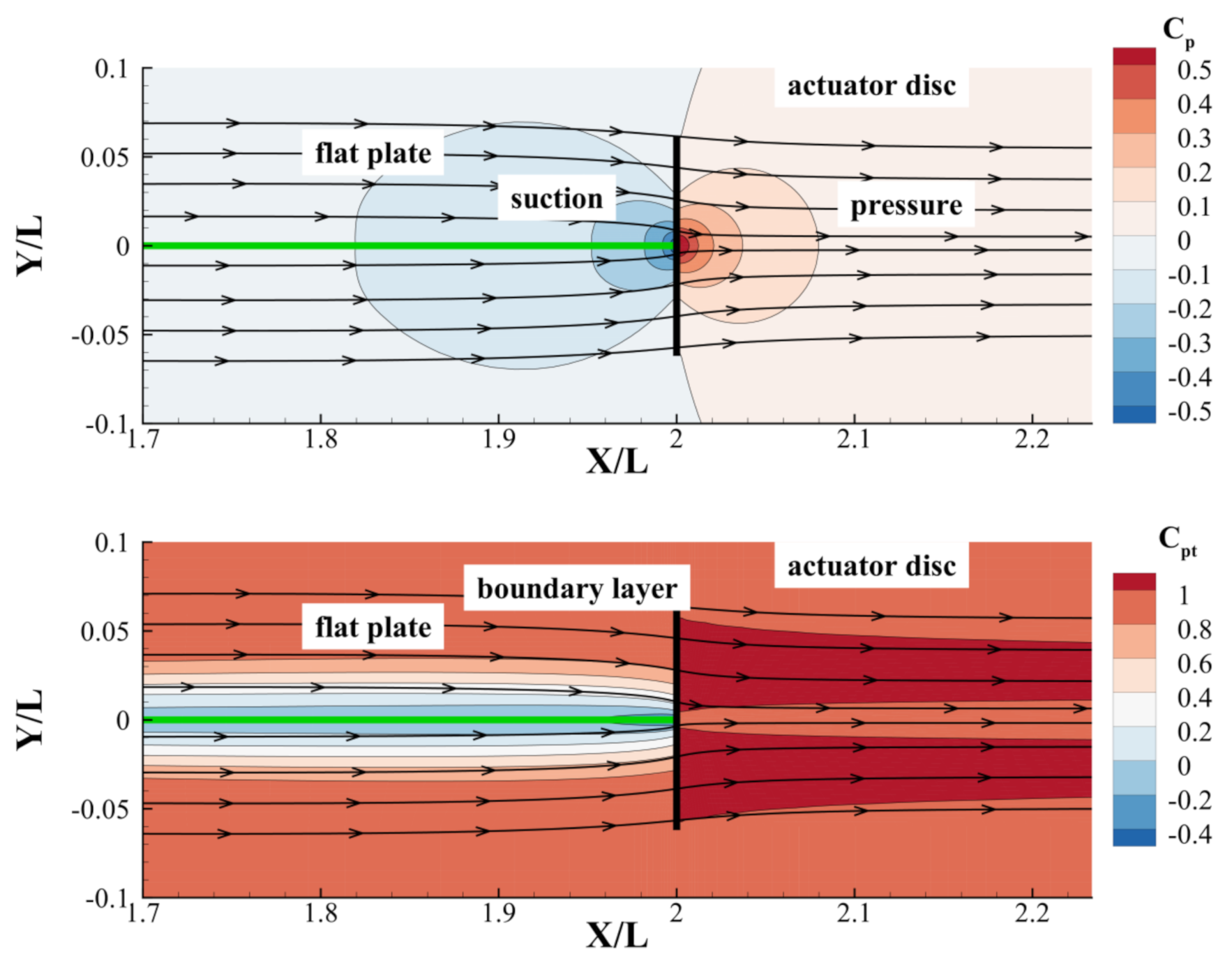
3.3. An Integrated Vehicle in Laminar Flow

This section presents a simulation study of an integrated vehicle combining a flat plate with a wake filling actuator disc model in a BLI configuration. This combination of elementary models is beneficial for analyzing the mechanisms of BLI. The CFD simulation of the vehicle uses the computational domain shown in Figure 6. An actuator disc is placed at the TE of the plate, such that the actuator disc model is ingesting the boundary layer. The boundary condition of the flat plate is kept as a non-slip wall condition.

$$∆p\left(y\right) =∆p_t\left(y\right) =p_{t, const}-p_{t,upstr}\left(y\right)$$

(15)

An ideal model is introduced for the discussion of BLI mechanisms. The actuator disc ingests and advances the boundary layer flow in such a way that it perfectly refills the total pressure defect (Instead of velocity defect, total pressure defect is used because the jump of total pressure is identical to the static pressure jump of the actuator disc. This is attributed to the continuity of velocity through the actuator disc) of the boundary layer. This ideal model is also known as a wake filling actuator [13,24]. It is represented by a pressure jump plane with a non-uniform distribution of Δp. During the computation process of simulation, the value of Δp is updated through a User Defined Function (UDF). The Δp is obtained by subtracting a constant total pressure p_t,const with the total pressure p_t,upstr probed at an upstream plane in front of the actuator, as shown in Equation (15). The scheme of the wake filling actuator disc is illustrated in Figure 10. To maintain a perfect equilibrium (thrust T equals to drag D) is tricky in this simulation, thus p_t,const is defined to be slightly higher than p_t∞ in the UDF. This leads to the thrust T being higher than the drag D (the net force N defined in Equation (17) is slightly higher than zero).

CFD simulation is performed for the integrated vehicle model with the same simulation conditions as in the previous cases. Simulation results of the flow field around the wake filling actuator disk are shown in Figure 11. The top picture presents the contours of (static) pressure coefficient C_P. A notable phenomenon is that the flat plate is partially immersed in the suction region of the actuator model, creating a negative pressure gradient along the x-axis of the plate. This phenomenon supports the body/propulsor interaction discussed in reference [13]. Another phenomenon is the elliptical contours of C_P, whose center coincides with the center of the actuator model. This elliptical pattern is due to the non-uniform distribution of Δp. The bottom drawing of Figure 11 depicts the contours of the coefficient of total pressure C_Pt. The laminar contours of C_Pt over the flat plate denote the boundary layer. In the region behind the actuator disc, C_Pt is nearly uniform with a value slightly greater than 1. This shows that the wake filling actuator model fills the total pressure defect of the boundary layer, and energises the flow into the free stream condition.

The forces acting on the vehicle can be evaluated. The viscous drag D (0.0125 N) of the plate is obtained from the simulations. The T (0.0130 N) of the actuator disc is calculated by using Equation (16). The net force N (0.0005 N) is obtained by subtracting the drag D from the thrust T, as shown in Equation (17).

$$T={{\displaystyle ∯}}_{actuator}^{}∆p\left(y\right)dS$$

(16)

$$N=T-D$$

(17)

The power-based analysis is performed to study the power conversion process. The power balance equation for the vehicle is given in Equation (18) [13]. The input power of P_K (0.0936 W) is calculated with Equation (13). This value is the reference value for the normalization of all the involved power terms. The terms of output power are NV_∞ (0.005 W), energy flow rate Ė_w and viscous dissipation Φ.

$$P_K=N{V}_{\infty }+{\dot{E}}_w+\Phi$$

(18)

The top drawing in Figure 12 shows the integrand of Φ of the flow field. The high-intensity region corresponds to the boundary layer over the plate. Behind this boundary layer, the low-intensity region is notably different from the wake of the isolated plate. The bottom plot of Figure 12 illustrates the change of powers. The input power of P_K denotes the height of the shaded bar located at the same x position of the actuator model. The curves with different colours represent the output powers in Equation (18). This plot shows that the input power of P_K tends to be equal to (Φ + Ė_w + NV_∞), with the relative difference of 1.1% as the numerical error of the simulation. The error becomes larger when compared with the case of the isolated actuator disc (0.6%) or the flat plate (0.7%). This increase in numerical error might be caused by the UDF function that updates the value of the pressure jump in each iteration during computation. This unstable boundary condition defined by UDF potentially increases the error. The bottom plot depicts the power conversion of the integrated vehicle: the input power P_K primarily becomes the viscous dissipation boundary layer Φ_BL and the remaining part of P_K turns into NV_∞.

The bottom plot in Figure [12] shows a key feature in the power conversion of the vehicle. The energy flow rate of the boundary layer (wake) Ė_w (denoted by the gap between the red line and the blue line) is a transient power in the power conversion process: it keeps increasing from the LE until the TE and then abruptly drops to zero at the region behind the TE. The prompt drop of Ė_w is caused by the actuator that reenergises the boundary layer (wake) flow into the free stream condition. A previous study on mechanisms of BLI states that the power saving is due to the elimination of the power pertaining to the wake [8]. This study shows that the input power of the integrated vehicle P_K (0.0936 W) is reduced as compared with the power in the case of flat plate DV_∞ (0.1064 W). The power saving due to BLI is 13.7% (P_K as the reference value). On the other hand, the vehicle almost eliminates the wake power Ė_w, whose value is 20.1% of P_K. Results indicate a −6.4% difference between the quantity of power saving and the value of eliminated Ė_w. In this study, the error of power imbalance is 1.1%, too small to be responsible for this difference. On the other side, NV_∞ is a useful output power accelerating the vehicle. The ratio of NV_∞ over P_K is 3.6%, relatively close to the difference. It is reasonable to consider that NV_∞ benefits from the reduction in wake power. In short, this study supports the mechanism that the elimination of wake power leads to power saving, and it also shows that wake elimination could cause a benefit of generating net force power.

A previous theoretical study elaborates the cause of propulsive coefficient η_p (“propulsive efficiency” is not a strictly defined efficiency in the case of BLI, this figure of merit is called “propulsive coefficient” to avoid confusion in this study) exceed unity for a BLI propulsor [13]. It is noted that the definition of this figure of merit is identical to that of the propulsive efficiency, whose value is in the range of 0.7~0.8 for a modern turbofan engine. This simulation obtains the propulsive coefficient η_p value of 1.38, slightly higher than the value of 1.27 given in the previous theoretical study, which actuator disc ideally refills the wake of a flat plate. The higher value η_p in this study might be attributed to another mechanism of BLI ignored in the previous study: the aerodynamic interaction between body and propulsor. In the BLI configuration, the suction side of the actuator introduces a negative pressure gradient in the vicinity of TE, as can be seen from the top plot in Figure 11. This pressure gradient accelerates the boundary layer flow. On the other hand, the velocity at the bottom of the boundary layer is kept at zero due to the non-slip wall condition; consequently, the velocity gradient at the wall (skin friction) increases. As a result, the drag increases as compared with the isolated flat plate. To maintain thrust drag equilibrium, a higher thrust is required to balance this drag increment in this case, thereby leading to a higher value of η_p. In general, this aerodynamic interaction increases viscous drag and changes the viscous dissipation of the boundary layer. This simulation study provides numerical evidence for the body/propulsor interaction. Results show that the C_d of the plat in the integrated vehicle (0.020407) is increased by 17.5%, as compared with the C_d value of the isolated plate (0.017374). As for the change in viscous dissipation of the boundary layer, the interaction increases Φ_BL of the vehicle by 8.6%, compared with the value in the case of the flat plate in isolation.

4. Power Bookkeeping in Turbulent Flows

This section discusses power-based analysis in turbulent flows. The physical process involved in turbulent flow poses challenges to numerical simulations, and time averaged (Reynolds averaged) methods are usually adopted to simplify turbulence issues. This study employs steady Reynolds Averaged Navier–Stokes (RANS) simulations and a two-equation k-ω-sst turbulence model to simulate turbulent flows. In this turbulence model, turbulent viscosity μ_tur and turbulent dissipation rate e are given by Equation (19); k stands for the turbulent kinetic energy, whereas ω is the specific dissipation rate of the turbulence model [25]. Due to the energy conservation involved in the turbulence model, it is possible to study the power conversion from the mechanical energy of mean flow to the energy of turbulent flows. The following paragraphs elaborate power bookkeeping of typical models in turbulent flows. For the interest of mechanisms involved in BLI, two cases of a flat plate and a BLI-integrated vehicle are studied accordingly.

$${\mu }_{tur}=\rho \frac{k}{\omega } , e=k\omega$$

(19)

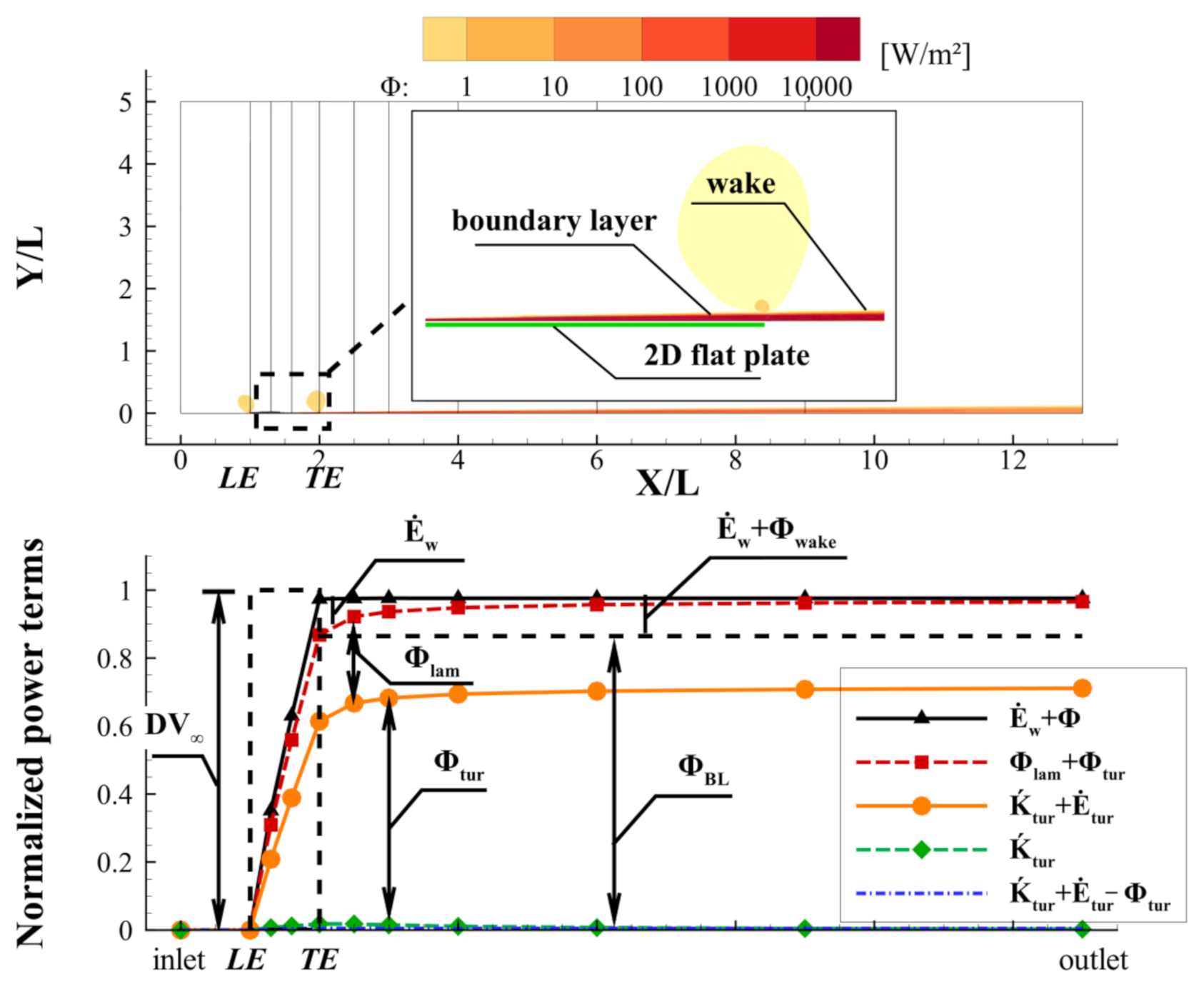
4.1. Flat Plate in Turbulent Flow

This part discusses the case of turbulent flow over a 2D flat plate. In the simulation of this case, the Reynolds number is set to 10 million such that the viscous flow is fully turbulent. Numerical simulation utilizes the common computational domain in which boundary conditions are set corresponding to the case of a flat plate. It is noted that the size of the domain is scaled 100 times. Mesh density is increased in the viscous region with a total cell number of about 60,000. The mesh sensitive study indicates that simulations are grid independent in the cases of flat plate and integrated vehicle, as shown in

Table 4. Mesh sensitive study for turbulent simulations.

Case	Cell Number	Φ (Watt)	Relative Difference
Flat plate	6000	2075.95	59.5%
	60,696	5307.58	3.5%
	223,383	5165.54	0.7%
	877,608	5130.42	0.0%
Integrated vehicle	6000	1512.897888	67.7%
	60,696	4811.02	2.8%
	223,383	4698.036482	0.3%
	877,608	4682.1	0.0%

. The Y plus value in the boundary layer region is less than 5.

The power balance equation of a flat plate with turbulent flow remains the same as the in case of laminar flow (Equation (14)). To address turbulence issues, the viscous dissipation rate Φ in the equation can be further broken down into laminar viscous dissipation rate Φ_lam and turbulent viscous dissipation rate Φ_tur, as in Equation (20). The expression of Φ_tur adopts the Boussinesq hypothesis, as a product of e velocity gradient and turbulent viscosity. Furthermore, this study breaks down Φ_tur to analyze the power conversion of turbulent flow based on the energy conservation of a two-equation turbulence model. In the process of energy transfer in the turbulent flow, the energy of the mean flow is transferred to the kinetic energy of large eddies. Once the large eddies break into small eddies, the energy is dissipated within small eddies. The power balance equation of the turbulent model can be expressed as Equation (21). In this equation, turbulent kinetic energy flow rate Ḱ_tur denotes the kinetic energy that pertains to large eddies. The expression of Ḱ_tur applies surface integral as given in Equation (22). Turbulent energy dissipation rate Ė_tur refers to the energy dissipated in the small eddies; its expression uses volume integral as in Equation (23). It is noted that the k and e (epsilon) in Equations (22) and (23) denotes turbulent kinetic energy and turbulent dissipation rate in the two-equation turbulent model, respectively. This study utilizes k-ω-sst model to analyze the power conversion of the flat plate with turbulent boundary layer. A one-equation model (the Spalart–Allmaras model) is also tested as a reference, and the impacts of two turbulent models on the power-based analysis are briefly discussed.

$$\Phi ={\Phi }_{\mathrm{lam}}+{\Phi }_{\mathrm{tur}}\cong \underset{CV}{\overset{}{{\displaystyle \iiint }}}\left({\mu }_{lam}\frac{\partial u}{\partial y}-\rho u^{\prime }{v}^{\prime }\right)\frac{\partial u}{\partial y}dV=\underset{CV}{\overset{}{{\displaystyle \iiint }}}\left({\mu }_{lam}+{\mu }_{tur}\right){\left(\frac{\partial u}{\partial y}\right)}^{2}dV$$

(20)

$${\Phi }_{\mathrm{tur}}\cong {\dot{K}}_{tur}+{\dot{E}}_{tur}$$

(21)

$${\dot{K}}_{tur}=\underset{SP}{\overset{}{{\displaystyle \iint }}}\rho u kdS$$

(22)

$${\dot{E}}_{tur}=\underset{CV}{\overset{}{{\displaystyle \iiint }}}\rho edV$$

(23)

Steady RANS simulation with k-ω-sst model is performed for the case of the flat plate. The second-order upwind scheme for spatial discretization and the SIMPLE scheme for the pressure-velocity coupling are employed in this simulation. The results of the simulation are processed through power-based analysis. The top plot in Figure 13 illustrates the integrant of Φ (including laminar and turbulent contributions). The high-intensity region indicates the boundary layer over the plate as well as the downstream wake. It is noted that low-intensity region of Φ over the flat plate is observed in the laminar boundary layer over the plate. The low-intensity region is missing in this turbulent case because the intensity of turbulent dissipation is significantly higher than the laminar one. The bottom part of Figure 13 illustrates the power bookkeeping of the flat plate in turbulent flow. All the power terms are normalized by taking DV_∞ as a reference value. The input power DV_∞ is denoted by the height of the dashed lined- rectangular in the plot. The output power consists of the energy flow rate of wake Ė_w, laminar viscous dissipation rate Φ_lam and turbulent viscous dissipation rate Φ_tur. It is noted that the error of power imbalance is 2.3%, which is about 3 times larger than the error (0.7%) in the case of laminar flow. The increase in the error might be caused by the turbulent model which adds an extra energy transfer process in the power-based analysis. In this case, the viscous dissipation in the boundary layer Φ_BL (Φ at the TE) takes up 87.1% of the input power. This means the portion of wake power is 10.6%, lower than that in the case of laminar flow.

In the power bookkeeping of the plate, the bottom plot in Figure 13 shows that laminar viscous dissipation Φ_lam (the distance between the red line and the orange line) takes about 26.0% of the total power at the outlet, whereas turbulent viscous dissipation Φ_tur (orange line) is about 70.6% of the total power. The high percentage of Φ_tur might be attributed to the high Reynolds number (10 million) in the simulation. The bottom plot illustrates that Φ_tur keeps increasing along the x axis, whereas the value of Φ_lam increases from the LE to the TE, showing that laminar flow only exists in the boundary layer. It is noted that Φ_tur can be further broken down. The blue dotted line in the plot represents the error of power imbalance in turbulence flow (Ḱ_tur + Ė_tur − Φ_tur), whose value is about 0.5%. This plot illustrates that turbulent energy dissipation rate Ė_tur (the distance between the orange line and the green line) is the major component of Φ_tur and its value is about 99.6% of Φ_tur at the outlet. On the other hand, there is only a small portion (less than 2.5% of Φ_tur) of turbulent kinetic energy flow rate Ḱ_tur (green line) in the vicinity of TE, and this power is quickly dissipated in the downstream wake. This indicates that the Ḱ_tur (corresponds to large eddies) is quickly exhausted in the turbulent flow.

This work studies the 2D flat plate in laminar and turbulent flow conditions.

Table 5. Results of the 2D flat plate.

	Cd	(Ew/DV∞)TE
k-ω-sst model simulation	0.002879	10.8%
S-A model simulation	0.003101	10.2%
Schlichting’s solution	0.0031	-
Laminar simulation	0.017374	23.5%
Blasius’ solution	0.016045	-

lists the results of different models of the plate, namely RANS with the k-ω-sst model, RANS with the S-A model, Schlichting’s flat plate with fully turbulent boundary layer [26], laminar simulation, and Blasius’ laminar solution. This table shows that simulation results of drag coefficient C_d are close to theoretical solutions: differences are less than 7% for turbulent cases (referred to the Schlichting’s solution 0.0031), and less than 6% for laminar cases (referred to the Blasius’ solution 0.016045). As for the wake power, the percentage of Ė_w in turbulent flow takes about 46.0% of the value in the laminar case. This reduction of wake power in turbulent flow is attributed to the generation of power in turbulent flows. Results show that the difference between turbulent models leads to a moderate change: the one-equation S-A turbulent model causes a 7.2% increase in C_d and a 5.9% decrease in the percentage of Ė_w, as compared with the k-ω-sst model. Nevertheless, the one-equation model is incapable of breaking down Φ_tur, therefore, it is left without further discussion. This study adopts the k-ω-sst model for power-based analysis because the energy conservation of this model supports breaking down the power in the turbulent flow. If simulations adopt alternative two-equation turbulent models, for instance, the k-e models, the power-based analysis remains the same, as elaborated in this study.

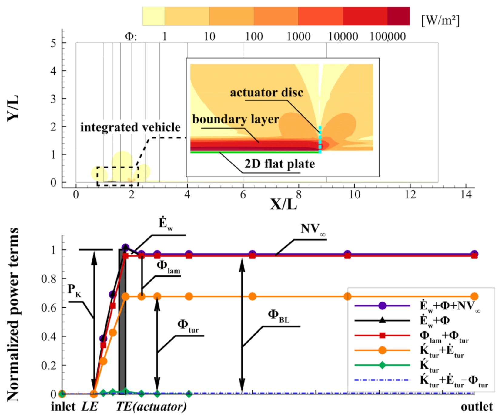
4.2. An Integrated Vehicle in Turbulent Flow

This part discusses the BLI-integrated vehicle in turbulent flow. Flow conditions in the simulation of the vehicle are the same as in the previous case in turbulent flow. The common computational domain is used with its boundary conditions corresponding to the integrated vehicle. RANS simulation with the k-ω-sst model is performed, and a UDF is introduced to represent the wake filling actuator disc. Simulation results are post processed through power-based analysis. It is noted that the power balance equation of BLI-integrated vehicles in turbulent flows can be expressed by Equation (18), the same as in the case of the vehicle in laminar flow. In this equation, viscous dissipationΦ could be breakdown into the components of Φ_lam and Φ_tur. Based on the energy conservation of the turbulent model, Φ_tur is further decomposed into turbulent kinetic energy flow rate Ḱ_tur and turbulent energy dissipation rate Ė_tur.

Figure 14 presents the simulation results of the BLI-integrated vehicle. The top plot depicts the intensity of Φ. As can be seen from this plot, highly intensive dissipation only occurs in the boundary layer over the plate. The intensity of Φ is significantly reduced in the downstream region behind the TE, showing that the actuator disc refills the energy defects of boundary layer flow and eliminates wake dissipation. The bottom plot of Figure 14 presents power bookkeeping of the vehicle. P_K is represented by the height of the grey rectangle, and it is the reference value for the normalization of all the involved power terms. The imbalance between input power P_K and out power (Ė_w + Φ + NV_∞) is 3.1%, slightly higher than the error in the case of the flat plate in turbulent flow. Results show that only 1.3% input power is transferred into net force power NV_∞, indicating the vehicle is close to the equilibrium state. The remaining 98.7% of the input power is converted into the viscous dissipation in the boundary layer Φ_BL in which 28.6% is due to Φ_lam and 67.0% is due to Φ_tur. To breakdown the viscous loss due to turbulences, turbulent kinetic energy flow rate Ḱ_tur only takes a small percentage (Ḱ_tur/Φ_tur), no more than 2.8% of Φ_tur in the vicinity of TE, whereas the turbulent energy dissipation rate, Ė_tur, mainly contributes to the power loss of Φ_tur within the flow field.

Simulation results enable the analysis of power saving due to BLI. the input power of the BLI vehicle (P_K) is 9.3% lower than the power of the flat plate in isolation (DV_∞). On the other side, the elimination of Ė_w at the TE is only 5.8% of P_K. In this case, power saving is higher than the reduction of wake power, this indicates alternative sources other than wake elimination reduce the power consumption of the vehicle. This result does not support the mechanism of BLI that the elimination of wake power leads to the power saving of BLI. An inspection can be made by checking the error of power imbalance (Ė_w + Φ + NV_∞ − P_K). This error is −3.1%, close to the difference, and the negative value of this error has the tendency to reduce the input power in the power balance equation. As a result, it is reasonable to consider that the numerical error is responsible for the difference between the power saving and the elimination of wake power.

This study assesses the propulsive coefficient of the wake filling actuator to be 1.12. Similar to the case of the vehicle in laminar flow, the negative pressure gradient in the vicinity of TE can be found in this case. In principle, this indicates the aerodynamic interaction between body and propulsor. Nevertheless, turbulent flow simulations show that the increase in Φ_BL (0.03%) and the drag coefficient increment C_d (1.2%) are not significant compared with the 3.1% simulation error.

5. Conclusions

The study presented in this paper introduces a power-based analysis of post process simulation results. Laminar and turbulent flow simulations are performed to study the mechanisms of BLI. Power terms are quantified to study the typical power conversion in the flow field. This study illustrates the processes of typical power conversion in a jet, an actuator disc, a flat plate, and an integrated system in BLI configuration. These power conversions provide numerical evidence to study the mechanisms involved in BLI. The main findings of this work are presented as follows:

• The error of power imbalance between input and output is associated with the numerical error of simulations. It depends on the complexity of the simulation. For instance, the introduction of UDF and turbulent model tends to increase the error. In this study, the smallest error is 0.26% in the case of laminar jet, whereas the largest error is 3.1% in the case of BLI-integrated vehicles in turbulent flow.
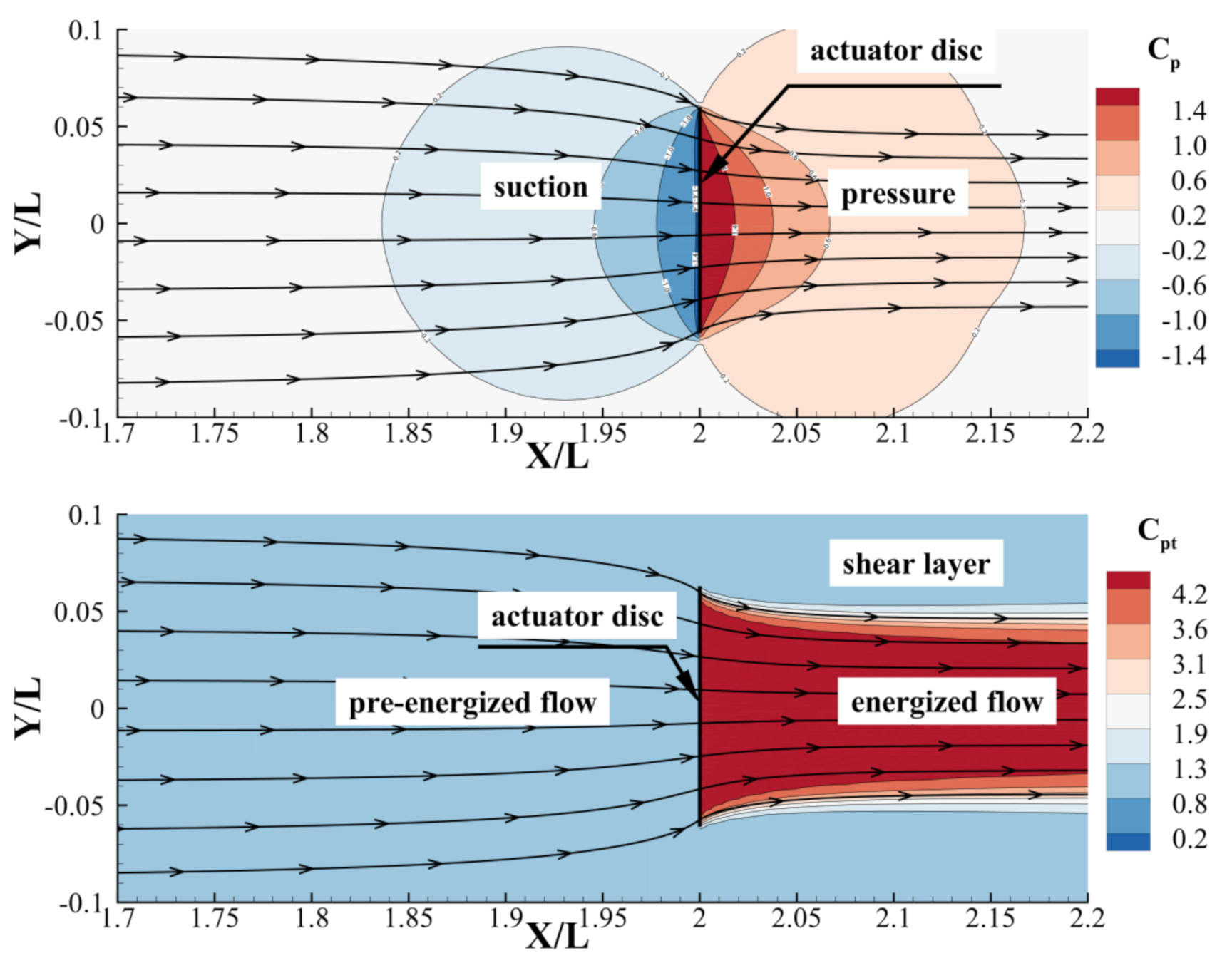
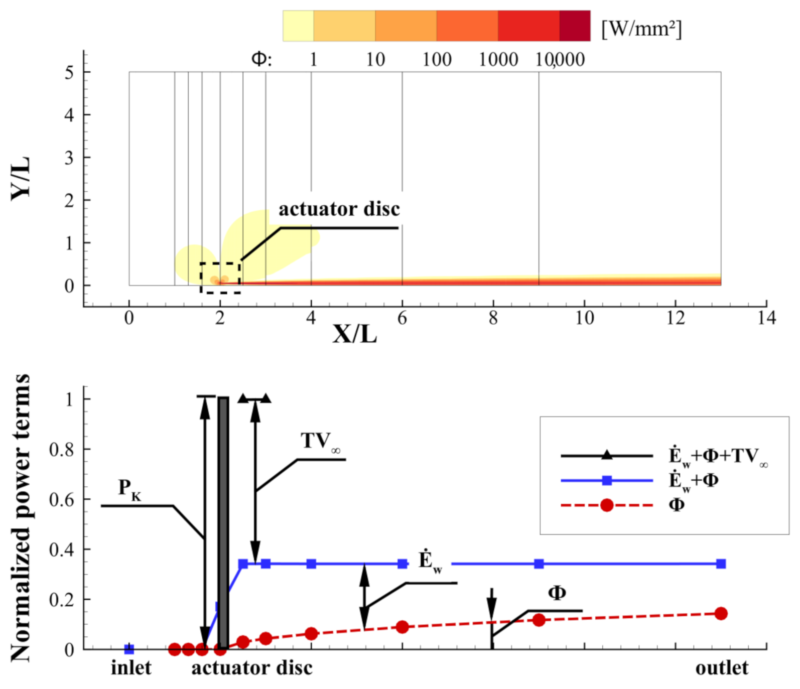
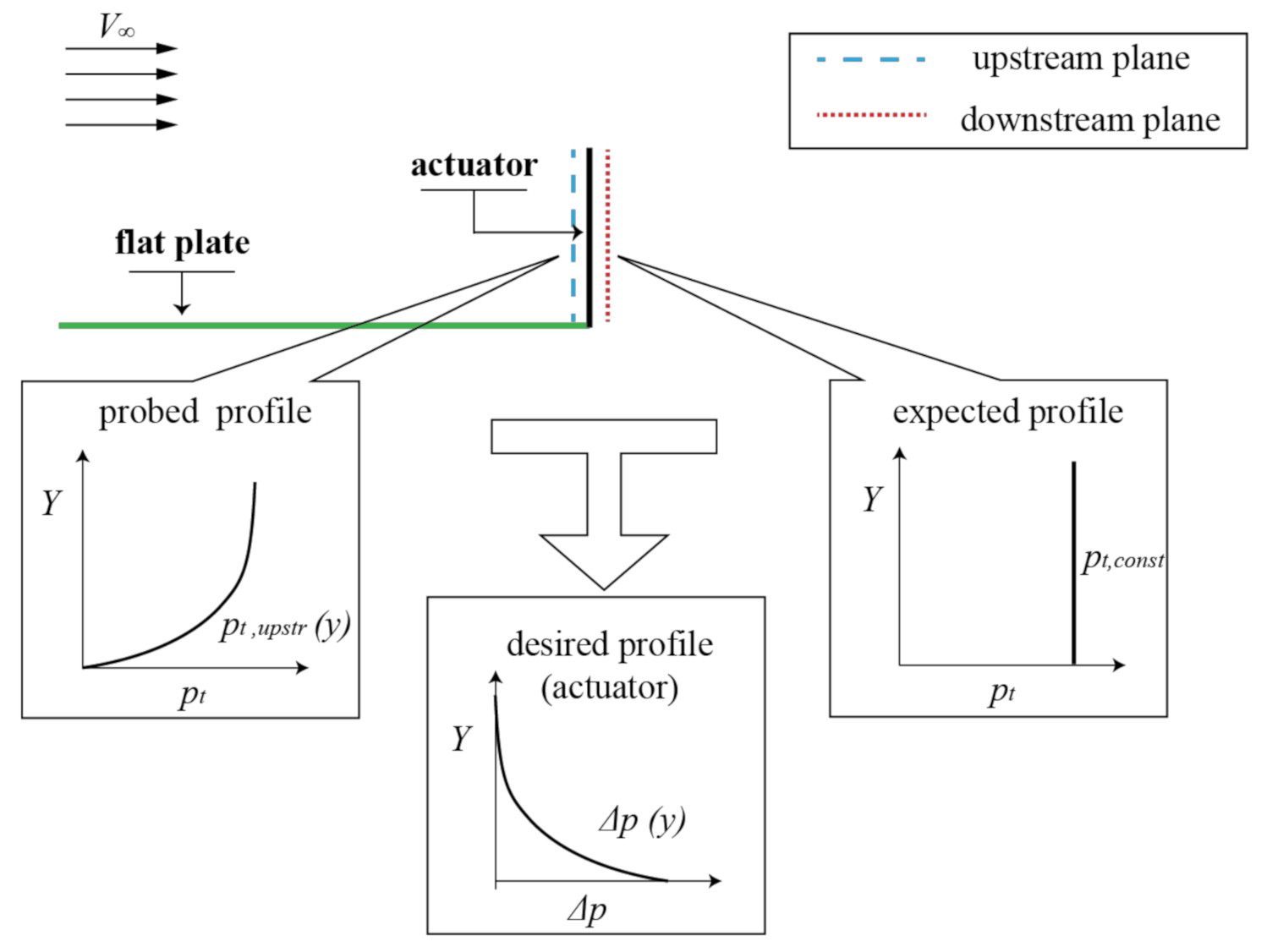
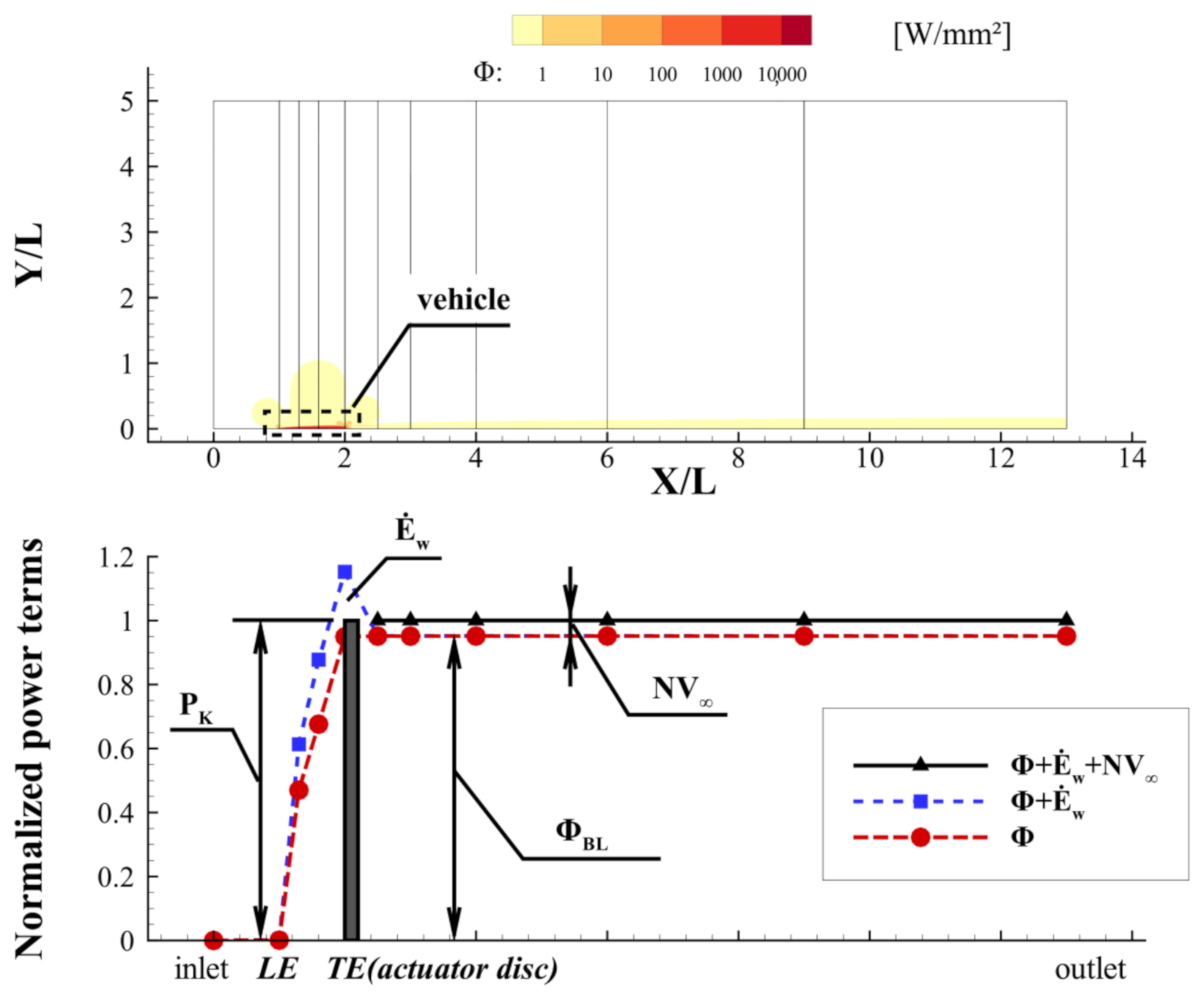
• This study validates the power-based method, illustrating typical processes of power conversion in the study of BLI. The actuator disc model represents a typical propulsor which converts input power P_K into thrust power TV_∞, energy flow rate of jet Ė_w at the outlet plane, and viscous dissipation Φ within the control volume. The simulation shows that the ratio between TV_∞ and input power is 65.4%, as a propulsive efficiency; 2D flat plate represents a body which converts the input power DV_∞ into viscous dissipation in boundary layer Φ_BL and energy flow rate of wake Ė_w. Results show that the ratio of Ė_w to DV_∞ is about 23.5% in laminar flow and 10.8% in turbulent flow; The integrated vehicle denotes a BLI configuration aircraft that translates input power P_K into net force power NV_∞, energy flow rate Ė_w at the outlet plane and viscous dissipation Φ within the control volume. It shows that Ė_w keeps increasing along the x axis in the boundary layer and is promptly eliminated through a wake filling actuator disc. Ė_w as a transient power causes the propulsive coefficient larger than unity. The propulsive coefficient of the wake filling actuator disc is 1.38 in laminar flow and 1.12 in turbulent flow.
• The mechanism of BLI saving power is due to the elimination of the energy flow rate of the wake. Laminar flow simulations show that the integrated system could save power consumption by 13.7% (with regard to the plate in isolate), slightly lower than the elimination of wake power (20.1%). The difference between power saving and wake elimination is due to the generation of the net force power NV_∞ of the vehicle (3.6%). Turbulent flow simulations show that the power saving due to BLI is 9.3%. This value is lower than the saving in the laminar flow because the portion of available wake power is reduced. Results show that the elimination of wake power (5.8%) is less than the power saving, the missing part of power saving can be attributed to the simulation error of power imbalance (3.1%).
• The aerodynamic interaction between body and propulsor is evidenced by the negative pressure gradient in the vicinity of TE. This interaction accelerates the flow in the boundary layer, therefore, changing the skin friction of the plate and viscous dissipation in the boundary layer Φ_BL. Laminar flow simulations show that the skin friction of the plate is increased by 17.5%, Φ_BL is increased by 8.6%. Turbulent flow simulations do not show the significant impact of interaction due to high simulation error.

This paper elaborates on an approach of power bookkeeping as the post processing of numerical simulation. The power terms which are essential in the discussion about mechanisms of BLI are evaluated in the flow field. This study shows although BLI increases airframe drag as a result of body/propulsor interaction, it saves power consumption overall due to wake elimination. For aircraft design which must integrate the airframe and the propulsion system, the pursuit of minimum power consumption rather than airframe drag is the goal for the least fuel consumption of the overall aircraft system.

References

1. Daggett, D.L.; Kawai, R.; Geiselhart, K.A. Blended Wing Body Systems Studies: Boundary Layer Ingestion Inlets with Active Flow Control; NASA: Washington, DC, USA, 2003.
2. Plas, A.; Crichton, D.; Sargeant, M.; Hynes, T.; Greitzer, E.; Hall, C.; Madani, V. Performance of a Boundary Layer Ingesting (BLI) Propulsion System. In Proceedings of the 45th AIAA Aerospace Sciences Meeting and Exhibit, AIAA Paper 2007-450, Reno, NV, USA, 8–11 January 2007. [Google Scholar]
3. Felder, J.; Hyun, K.; Brown, G. Turboelectric Distributed Propulsion Engine Cycle Analysis for Hybrid-wing-body Aircraft. In Proceedings of the 47th AIAA Aerospace Sciences Meeting, AIAA Paper 2009-1132, Orlando, FL, USA, 5–8 January 2009. [Google Scholar]
4. Uranga, A.; Drela, M.; Greitzer, E.; Titchener, N.; Lieu, M.; Siu, N.; Huang, A.; Gatlin, G.M.; Hannon, J. Preliminary Experimental Assessment of the Boundary Layer Ingestion Benefit for the D8 Aircraft. In Proceedings of the 52nd Aerospace Sciences Meeting, AIAA Paper, National Harbor, MD, USA, 13–17 January 2014. [Google Scholar]
5. Uranga, A.; Drela, M.; Hall, D.K.; Greitzer, E.M. Analysis of the Aerodynamic Benefit from Boundary Layer Ingestion for Transport Aircraft. AIAA J. 2018, 56, 4271–4281. [Google Scholar] [CrossRef]
6. Hall, D.K.; Huang, A.C.; Uranga, A.; Greitzer, E.M.; Drela, M.; Sato, S. Boundary Layer Ingestion Propulsion Benefit for Transport Aircraft. J. Propul. Power 2017, 33, 1118–1129. [Google Scholar] [CrossRef]
7. McClain, M. SAE Standard AIR4065A; Propeller/Propfan in-Flight Thrust Determination; SAE International: Warrendale, PA, USA, 2012. [Google Scholar]
8. Drela, M. Power Balance in Aerodynamic Flows. AIAA J. 2009, 47, 1761–1771. [Google Scholar] [CrossRef] [Green Version]
9. Arntz, A.; Atinault, O.; Merlen, A. Exergy-Based Formulation for Aircraft Aeropropulsive Performance Assessment: Theoretical Development. AIAA J. 2015, 53, 1627–1639. [Google Scholar] [CrossRef] [Green Version]
10. Arntz, A.; Atinault, O. Exergy-Based Performance Assessment of a Blended Wing–Body with Boundary-Layer Ingestion. AIAA J. 2015, 53, 3766–3776. [Google Scholar] [CrossRef]
11. Arntz, A.; Couilleaux, A.; Luquet, D.; Julienne, F. On the Use of Exergy as a Metric for Performance Assessment of CFD Turbomachines Flows Preliminary applications in Safran Aircraft Engines. In Proceedings of the 19th ISABE Conference, Canberra, Australia, 7−11 September 2019. [Google Scholar]
12. Lv, P.; Ragni, D.; Hartuc, T.; Veldhuis, L.; Rao, A.G. Experimental Investigation of the Flow Mechanisms Associated with a Wake-Ingesting Propulsor. AIAA J. 2017, 55, 1332–1342. [Google Scholar] [CrossRef]
13. Lv, P.; Rao, A.G.; Ragni, D.; Veldhuis, L. Performance Analysis of Wake and Boundary-Layer Ingestion for Aircraft Design. J. Aircr. 2016, 53, 1517–1526. [Google Scholar] [CrossRef]
14. Uranga, A.; Drela, M.; Greitzer, E.M.; Hall, D.K.; Titchener, N.A.; Lieu, M.K.; Siu, N.M.; Casses, C.; Huang, A.C.; Gatlin, G.M. Boundary Layer Ingestion Benefit of the D8 Transport Aircraft. AIAA J. 2017, 55, 3693–3708. [Google Scholar] [CrossRef] [Green Version]
15. Anderson, J.D.; Wendt, J.F. Discretization of Partial Differential Equations. In Computational Fluid Dynamics, 3rd ed.; Springer: Berlin, Germany, 2009; pp. 87–104. [Google Scholar]
16. White, F.M. Fundamental Equations of Compressible Viscous Flow. In Viscous Fluid Flow, 3rd ed.; McGraw-Hill: New York, NY, USA, 2006; pp. 59–95. [Google Scholar]
17. Panton, R.L. Incompressible Flow, 4th ed.; Willy: Hoboken, NJ, USA, 2013; pp. 205–207. [Google Scholar]
18. Sato, S. The Power Balance Method for Aerodynamic Performance Assessment. Ph.D. Thesis, Massachusetts Institute of Technology, Cambridge, MA, USA, 2012. [Google Scholar]
19. Lv, P. Theoretical and Experimental Investigation of Boundary Layer Ingestion for Aircraft Application. Ph.D. Thesis, Delft University of Technology, Delft, The Netherlands, 2019. [Google Scholar]
20. Versteeg, H.K.; Malalasekera, W. Solution Algorithms for Presure-Velocity Coupling in Steady Flows. In An Introduction to Computational Fluid Dynamics: The Finite Volume Method, 2nd ed.; Pearson: Harlow, UK, 2007; pp. 179–211. [Google Scholar]
21. Ansys Fluent Theory Guide; ANSYS, Inc.: Canonsburg, PA, USA, 2011.
22. Veldman, A. The Convection-Diffusion Equation. In Computational Fluid Dynamics; Institute for Mathematics and Computer Science: Groningen, The Netherlands, 2012; pp. 1–47. [Google Scholar]
23. Jasak, H. Error Analysis and Estimation for the Finite Volume Method with Applications to Fluid Flows. Ph.D. Thesis, Imperial College London, London, UK, 1996. [Google Scholar]
24. Smith, L.H. Wake Ingestion Propulsion Benefit. J. Propul. Power 1993, 9, 74–82. [Google Scholar] [CrossRef]
25. Menter, F.R. Two-equation Eddy-viscosity Turbulence Models for Engineering Applications. AIAA J. 1994, 32, 1598–1605. [Google Scholar] [CrossRef] [Green Version]
26. Schlichting, H.; Gersten, K. Boundary-Layer Theory; Springer: Berlin, Germany, 2017. [Google Scholar]
Figure 1. The diagram of the conservation of total energy and mechanical energy [19].
Aerospace 09 00184 g001
Figure 2. The diagram of power-based analysis to process the flow field of the simulation using the finite volume method [19].
Aerospace 09 00184 g002
Figure 3. Control volume definition and domain division [19].
Aerospace 09 00184 g003
Figure 4. A jet flow (top) and the definition of the computational domain (bottom) [19].
Aerospace 09 00184 g004
Figure 5. Contours of the integrand of viscous dissipation (top) and the power bookkeeping of the jet (bottom) [19].
Aerospace 09 00184 g005
Figure 6. A common computational domain for an actuator disc, a flat plate, and an integrated vehicle model [19].
Aerospace 09 00184 g006
Figure 7. Contours of pressure coefficient (top) and the coefficient of total pressure (bottom) around an actuator disc, including a mirrored flow field [19].
Aerospace 09 00184 g007
Figure 8. Contours of the integrand of viscous dissipation (top) and the power bookkeeping of the actuator disc (bottom) [19].
Aerospace 09 00184 g008
Figure 9. Contours of the integrand of viscous dissipation (top) and the power bookkeeping of a flat plate (bottom) [19].
Aerospace 09 00184 g009
Figure 10. The scheme of a wake filling actuator model [19].
Aerospace 09 00184 g010
Figure 11. Contours of pressure coefficient (top) and the coefficient of total pressure (bottom) around the wake filling actuator disc, including a mirrored flow field [19].
Aerospace 09 00184 g011
Figure 12. Contours of the integrand of viscous dissipation (top) and the power bookkeeping of the integrated vehicle (bottom) [19].
Aerospace 09 00184 g012
Figure 13. Contours of the integrand of viscous dissipation (top) and the power bookkeeping of the 2D flat plate (bottom) in turbulent flow (steady RANS with k-ω-sst model).
Aerospace 09 00184 g013
Figure 14. Contours of the integrand of viscous dissipation (top) and the power bookkeeping of the integrated vehicle in turbulent flow (bottom).
Aerospace 09 00184 g014