1. Introduction
Asteroids are the next frontier for space exploration. From revealing the mysteries of our solar system to potentially becoming a source of invaluable resources, asteroid-related topics are quickly acquiring major importance in space exploration. Recently, there have been several missions to asteroids. NASA recently launched Lucy, a fly-by mission to explore a record number of Trojan asteroids [
1]. JAXA is currently leading with two launches to asteroids Ryugu and Itokawa with their spacecraft Hayabusa 1 and 2; both were designed to orbit and bring back samples from the asteroids [
2]. NASA also had a recent success with their mission to the asteroid Bennu with OSIRIS-REx [
3]. There is no doubt that in the future there will be more missions to our neighboring asteroids for scientific purposes, resource exploitation and hazard avoidance.
Due to the growing interest, researchers in this are field working towards developing autonomous systems that rely less on ground-in-loop communication and do not require extensive knowledge about the asteroid’s shape and the environment [
4]. From a guidance, navigation and controls perspective, there have been several efforts made to address some of the critical aspects of missions to asteroids, including improved control systems that can explore the asteroids autonomously [
5,
6,
7,
8,
9]. Currently, most of the control systems are split into three main categories: (1) adaptive control, where the control system either directly updates its gains based on some update law or indirectly estimates asteroid parameters online and generates controller gains [
10,
11]; (2) robust control, which requires bounds on disturbances [
12] (e.g., a sliding mode control was successfully designed to control the Hayabusa2 spacecraft on its way to the asteroid Ryugu [
13]); (3) optimal control, which is highly dependent on system knowledge and requires explicit information about the asteroid and spacecraft parameters. However, ideally, an optimal control is desired, due the limited amount of fuel in the spacecraft [
7].
Unlike other approaches that rely solely on the performance qualities of adaptive controls or the optimality of model predictive controls, this work combines the benefits of adaptive and optimal control systems. We call this novel system direct–adaptive model predictive control (DAMPC). We use MPC to generate optimal reference trajectories and control inputs. Then, we use the control inputs as a feed-forward control in conjunction with simple adaptive control (SAC). The goal is that the adaptive control handles the disturbances that MPC fails to account for. Another major advantage of using this formulation is that an online MPC is not required since the adaptive control keeps the spacecraft on the desired trajectory, thus making the system computationally efficient. Since the MPC requires a model of the system, we implemented MPC on the two-body approximation of the asteroid model. The two-body formulation in the asteroid frame only requires the mass and angular velocity of the asteroid, both of which are usually available prior to the mission [
14] and can be updated online as the spacecraft gets closer to the asteroid. It should be noted that the two-body model does not require the shape of asteroid, and it is a valid assumption since the mass of the asteroid can be estimated using light curve and orbital analysis prior to the mission.
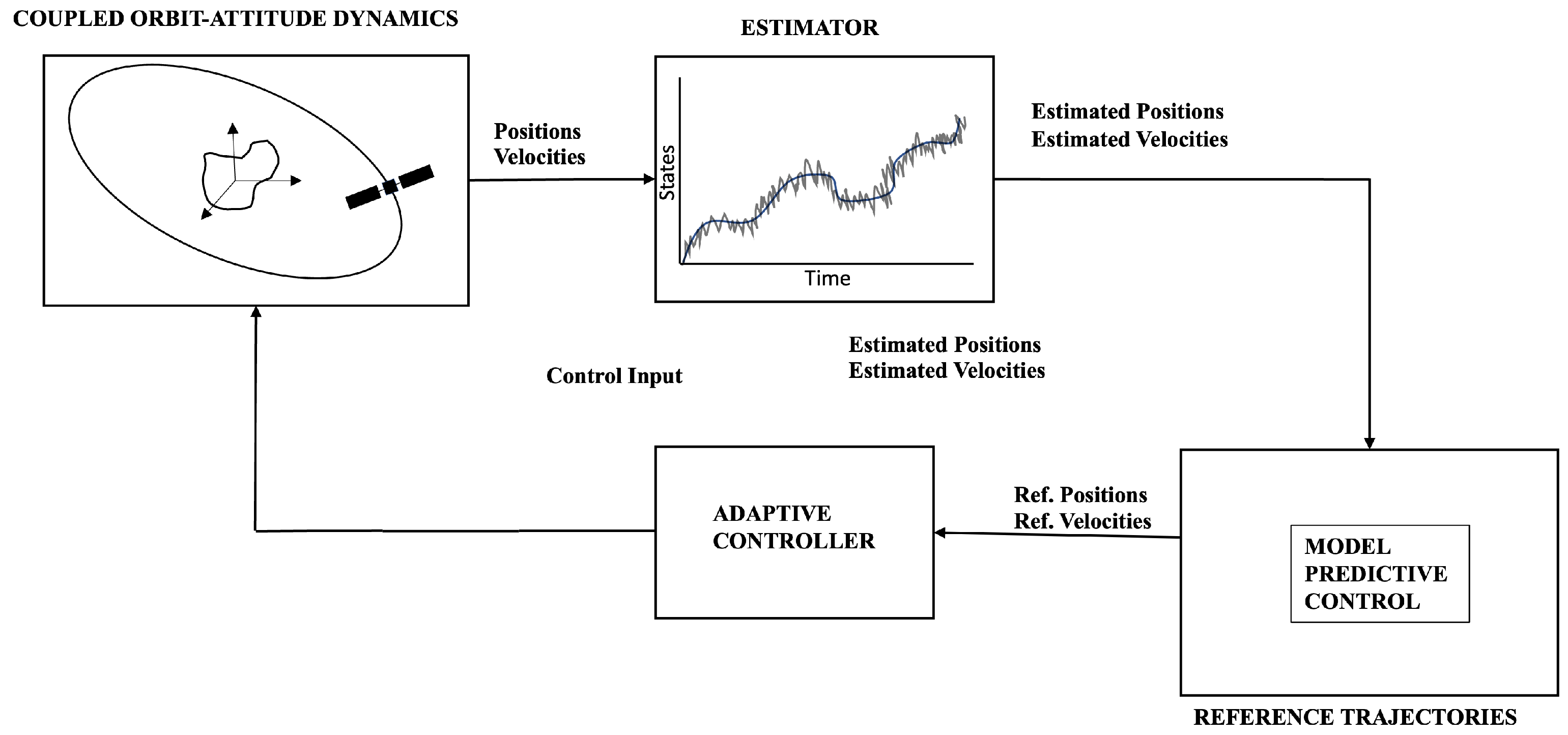
A schematic of DAMPC is shown in
Figure 1. It can be seen that the reference trajectory is generated using MPC. Then, the adaptive control is combined with feed-forward trajectories using MPC to control the actual spacecraft system. For the purposes of this paper, it is assumed that the estimated positions and velocities are readily available to the control system.
The paper is organized into the following sections.
Section 1 presents the dynamical formulation. In
Section 2, the DAMPC control formulation is discussed. In
Section 3, the simulation results are discussed. Finally, the work is concluded in
Section 4.
2. Dynamics
In this section, the dynamical formulation of the spacecraft is presented in the asteroid body frame. The gravitational field of the asteroid is modeled using a polyhedral gravity model for numerical testing with the DAMPC controller. However, for designing the MPC control, a two-body approximation of the model is considered.
The controlled spacecraft dynamics relative to the asteroid can be expressed in the rotating asteroid body fixed frame (
) as
where
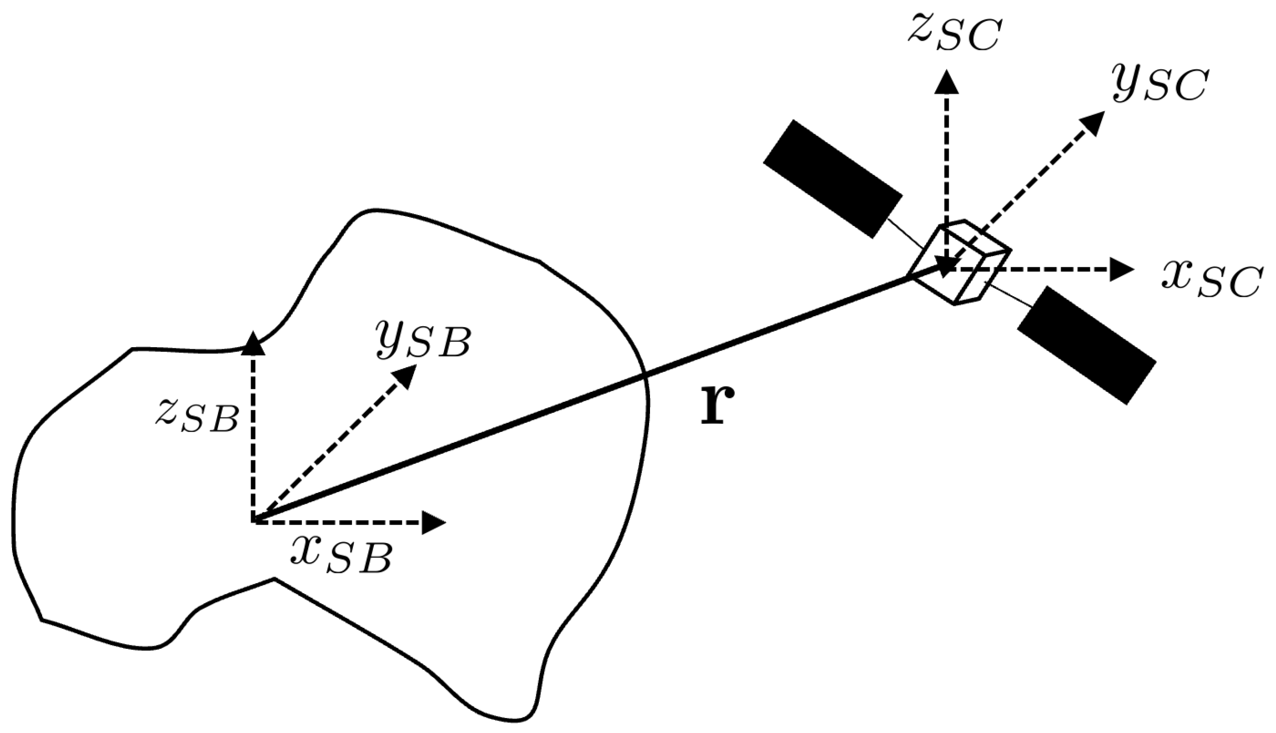
m is the mass of the spacecraft and
is the position vector from the center of mass of the asteroid to the center of mass of the spacecraft expressed in the asteroid body frame (
), as shown in
Figure 2. The angular velocity vector
is considered constant, where
is the magnitude of the angular velocity. The vector
is aligned with the unit vector
. Here,
is the force due to the polyhedral gravity model of the asteroid and
is the gravitational gradient force arising from the interaction between point mass gravity model of the asteroid and the rigid body model of the spacecraft. Furthermore,
is the force due to solar radiation pressure, which is dependent on the attitude of the spacecraft. The solar radiation pressure force
is modeled as a disturbance force to further test the performance of the DAMPC. Here,
is the thrust control vector assumed to be aligned with the principal axes of the asteroid.
A polyhedral gravity model was implemented to test the performance of the DAMPC control system. This model was proposed by Werner and Scheeres [
15]. The polyhedral model calculates the exact gravitational field for the given shape and density of the body. The main advantage of this model is that it does not diverge in the Brillouin sphere.
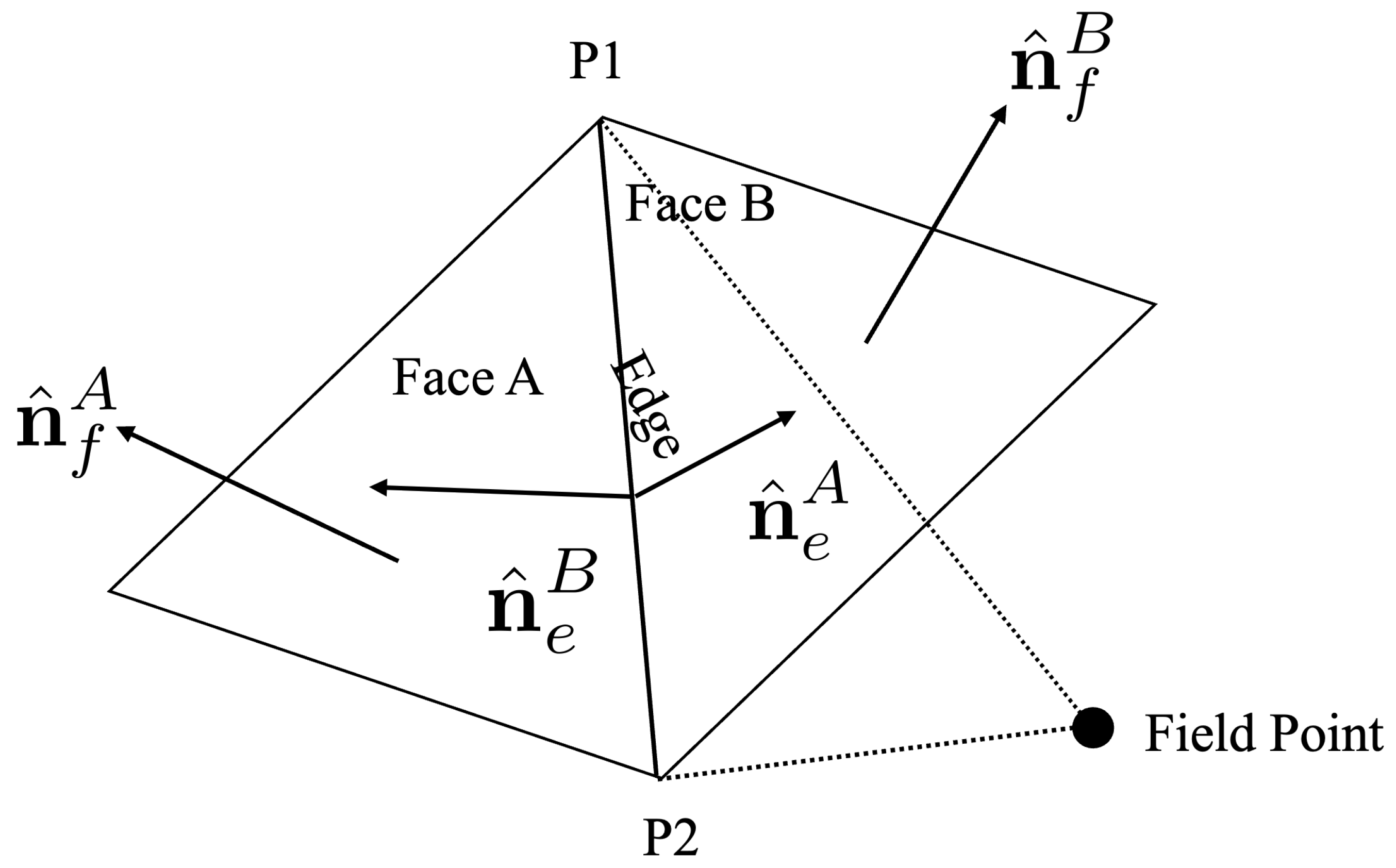
A polyhedral model was developed using a triangular facet with three vertices. Each edge of the facet is the boundary between two facets, as shown in
Figure 3. Here,
is the vector from the field point (spacecraft position in the asteroid body frame) to any point on the face plane. The vector
is a unit vector normal to the face plane. Each triangular facet is associated with its own coordinate frame (
), where
is aligned with the normal vector
. The vector
is a vector from the field point to any point at the edge
e. Each edge has a normal edge vector, which is normal to the edge vector
and the face normal vector
. Here, the edge vector
is the vector along the edge of the facet. Each edge is associated with two edge normal vectors (one for each face plane), namely
and
. The edge and face dyad constants are given as
The potential due to the edge is denoted by
and is given as
where ∥.∥ is the magnitude of the vectors. The dimensionless factor
is defined for each facet and is given as
where the vectors
,
and
are the vectors from the field point to each vertex of the triangular facet. Given the above-mentioned definitions, the acceleration due to the polyhedral shape of the body is given as
where
G and
are the gravitational constant and the density of the asteroid. The gravitational force (
) due to the polyhedral gravitational field of the asteroid on the spacecraft with mass
m is simply given as
The gravitational gradient force (
) is also added as a result of the rigid body shape of the spacecraft, as seen in
Figure 2. The gravitational gradient is modeled as a point mass gravity model of the asteroid. This is a reasonable assumption since the mission duration in this case is short [
16].
The force due to gravity gradient is given as [
17]
where
is the trace of the inertia tensor and
is an identity matrix.
The solar radiation pressure force is modeled using a flat model of the spacecraft. This model is similar to the model in Hayabusa2’s mission [
9]. The model is based on the assumption that the effect of SRP is primarily due to the solar panels. The SRP is modeled in the spacecraft body frame (
,
,
), as seen in
Figure 2. Without loss of generality, the solar panel is assumed to be perpendicular to the
axis. A vector
is defined as a unit vector parallel to the
axis. A sun-pointing vector (
) is defined as a vector pointing towards the the sun with respect to the spacecraft body frame.
The SRP force is dependent on the attitude of the spacecraft, which is modeled separately [
4]. The SRP force due to a flat plate model is given as [
9]
where
is the Lambertian coefficient,
A is the surface area of the flat plate and
is the SRP acting on the surface of the spacecraft. In addition,
and
correspond to optical constants of the spacecraft.
The two-body orbital dynamics equations that are implemented for the model predictive control are simply given as
where
and
are the position and velocity vectors of the spacecraft in Cartesian coordinates, respectively, and
is the thrust control vector. It is assumed that a six-thruster configuration is available for controlling the spacecraft in the configuration space.
3. Direct–Adaptive Model Predictive Controller
A direct–adaptive model predictive control (DAMPC) was implemented in this work. This formulation has two main advantages:
The adaptive control increases the robustness of the DAMPC since the system model for MPC is based on a low-fidelity gravitational model and other model disturbances are missing.
The MPC adds optimally to the control system via the feed-forward control inputs and generates sub-optimal trajectories to be fed into the adaptive control. In addition, the feed-forward control input initializes the control systems with a non-zero control input which helps to avoid overshoot caused by zero initial control input from the adaptive control.
This approach balances the effects of both adaptive and MPC control. Even though the NMPC is inherently adaptive, it cannot guarantee stabilizing the input for unknown model and system parameters [
18]. Therefore, the adaptive control increases the robustness of the MPC. In addition, adding MPC control inputs as feed-forward is more computationally efficient since the adaptive control converges faster than MPC and re-solving the optimal trajectory is only required if another obstacle is detected, which is unlikely in this case.
Any nonlinear dynamical system as given in Equation (
1) can be described in the following form [
19]:
where,
are the state, control and output vectors and
,
and
. It should be noted that in SAC, it is necessary to maintain the square state-space form; that is, the number of control inputs (
) must be equal to number of states being tracked (
) (i.e.,
).
The DAMPC system is based on a combination of a simple adaptive control system and model predictive control, i.e.,
The feedback control law
control is the robust modified version of the simple adaptive control [
4] given as
The update law for the gain
is based on the SAC [
20]. We implemented a robust modification based on work by Narendra [
21], to further account for noise in the system. The modified gain update law is given as
where
is a constant and
is the norm of the output tracking error. As the output tracking error tends to zero for an ideal tracking case, the
e modification term also tends to zero.
The output tracking error
is defined as
The feed–foward control law is designed using nonlinear model predictive control (NMPC) due the nonlinear nature of the constraints and equations. However, it should be noted that in the DAMPC formulation, a linear and convex MPC can also be implemented.
The nonlinear program for NMPC is given as
subject to:
where
and
are the current and desired states of the spacecraft. The prediction and control horizon length is given by
N. Q and R are the weighting matrices, which are manually tuned. The dynamical constraint is given in Equation (
19). The thrust constraint is given in Equation (
20). An ellipsoidal constraint was implemented in this work for obstacle avoidance, as given in Equation (
22) where
a,
b and
c are the half lengths of the principal axes of the ellipsoid. The ellipsoidal constraint can be seen in
Figure 4. It should be noted that a convex version of this constraint can also be implemented [
22]. A velocity constraint was also implemented, as shown in Equation (
21). It was necessary to include this constraint to avoid overshooting the trajectory. In our previous work [
4], we showed that the adaptive control guarantees asymptotic trajectory tracking for a system with square state-space form as given in Equation (
11). Therefore, the proposed control system converges for all initial conditions.
The term
is the cost of the final state and is defined here as
The equations of motion for NMPC are discretized using the fourth-order Runge–Kutta method and the nonlinear program is solved using a multiple shooting method.
4. Simulation and Results
The simulation is divided in to three sections. In
Section 1, we present the performance of feed-forward MPC to show that the feed-forward control is not sufficient to reach the desired state and a feedback control is needed due to the unknown irregular gravitational field and solar radiation pressure. In
Section 2, the performance of the simple adaptive controller without the feed-forward term is presented. The adaptive control is designed to track trajectories generated from the NMPC control. It is shown that even though the adaptive control is able to successfully track the trajectories, the control effort overshoots due to the zero initial condition for the adaptive control gains. In
Section 3, the performance of the DAMPC with and without noise is presented. It is shown that the DAMPC outperforms adaptive control in terms of noise handling and overall performance.
It should be noted that the MPC control in Equation (
10) uses estimated gravitational parameters, assuming that the true parameters are not available. The DAMPC system is applied to the full dynamics given in Equation (
1), assuming the gravity model is unknown. Although the gravity parameters for MPC could be subject to errors since they are estimated, the adaptive control can handle these errors, as shown in the following.
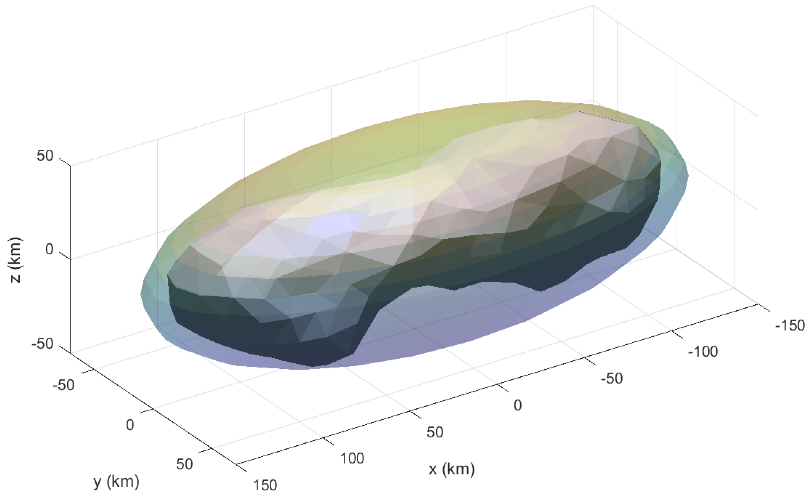
Asteroid Kleopatra was chosen for the simulation. The asteroid properties were taken from NASA’s Planetary Data System (PDS) [
23]. The properties of the asteroid and the spacecraft can be found in
Table 1 and
Table 2. Asteroid Kleopatra is a metallic ham-bone-shaped asteroid with a highly irregular gravitational field. The system dynamics were integrated using the Runge–Kutta fourth-order (RK-4) method with a time step of 1 s.
The initial and final position and velocity states are given as follows:
The NMPC conditions are given in
Table 3 for Case 2. The adaptive control gains were initialized with zero initial conditions and the adaptive tuning parameter was set to
.
4.1. Case 1: MPC Feed-Forward Only
In this section, the results for the case with NMPC only are presented. The NMPC is applied to the full system dynamics as given in Equation (
1).
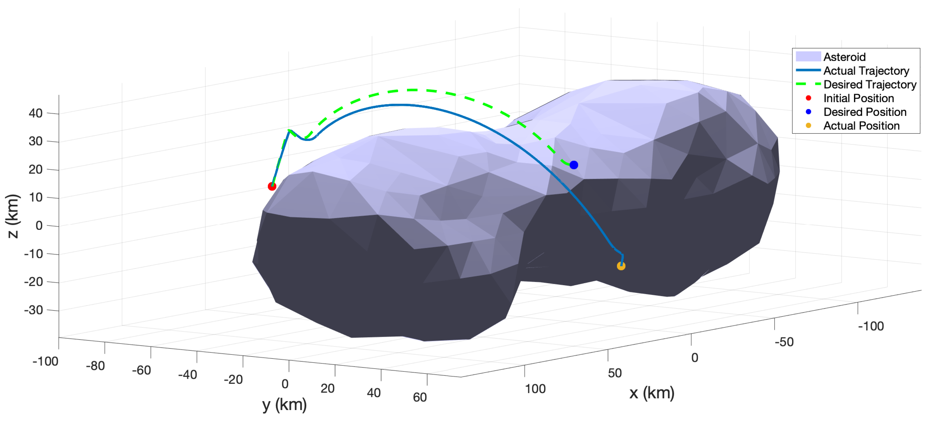
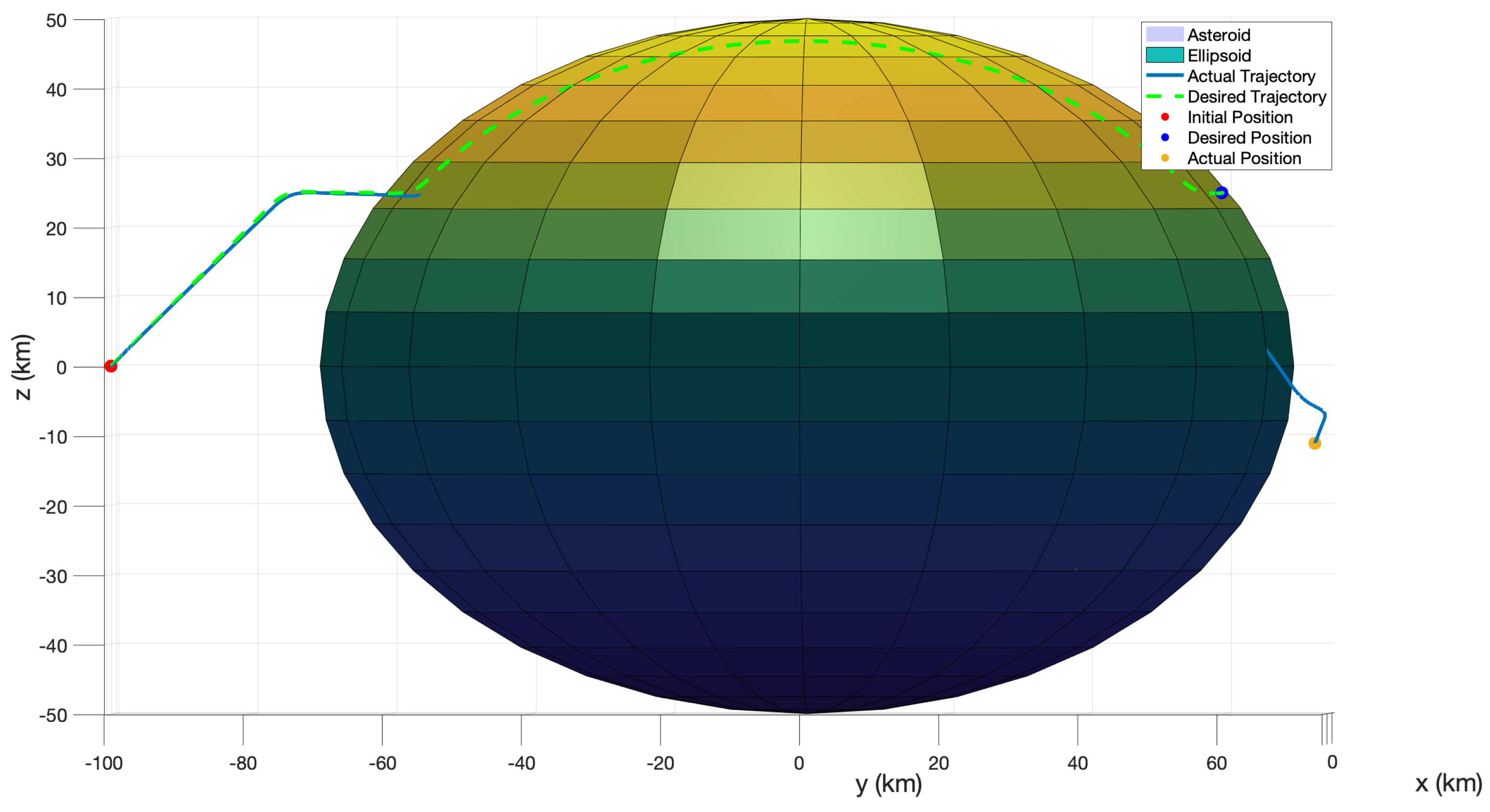
The desired and actual trajectories after implementing MPC feed-forward only can be seen in
Figure 5. In this case, it can clearly be seen that the trajectories diverge significantly. This is due to the fact that the NMPC control inputs are calculated using the two-body approximation of the system model as given in Equation (
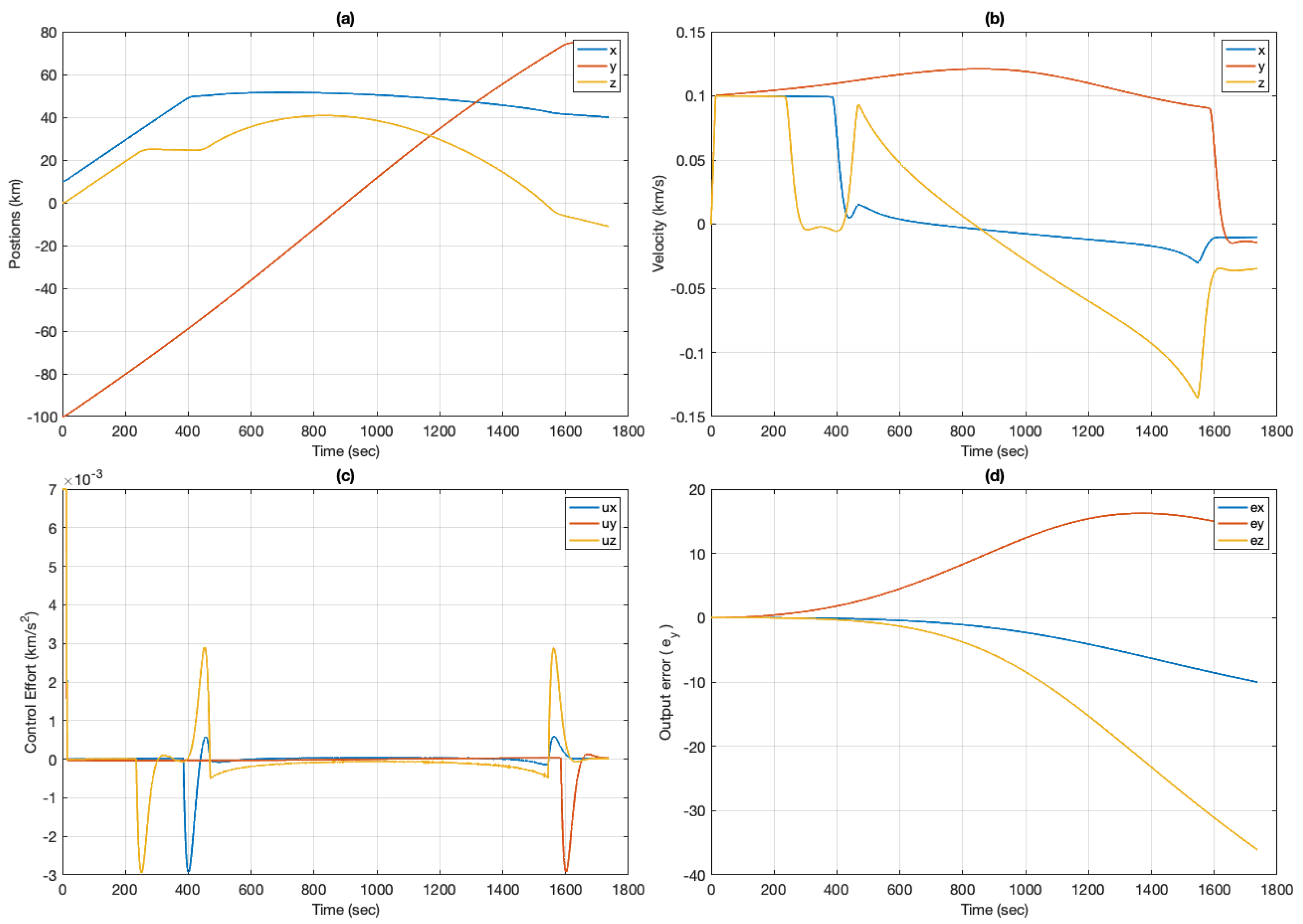
10). In the case of asteroid Kleopatra, the gravitational model is better represented by a polyhedral gravity model due to its highly irregular shape and total mass. In addition, as the duration of the mission becomes longer, the divergence from the desired position also increases and causes even more drift. The output error can be seen in
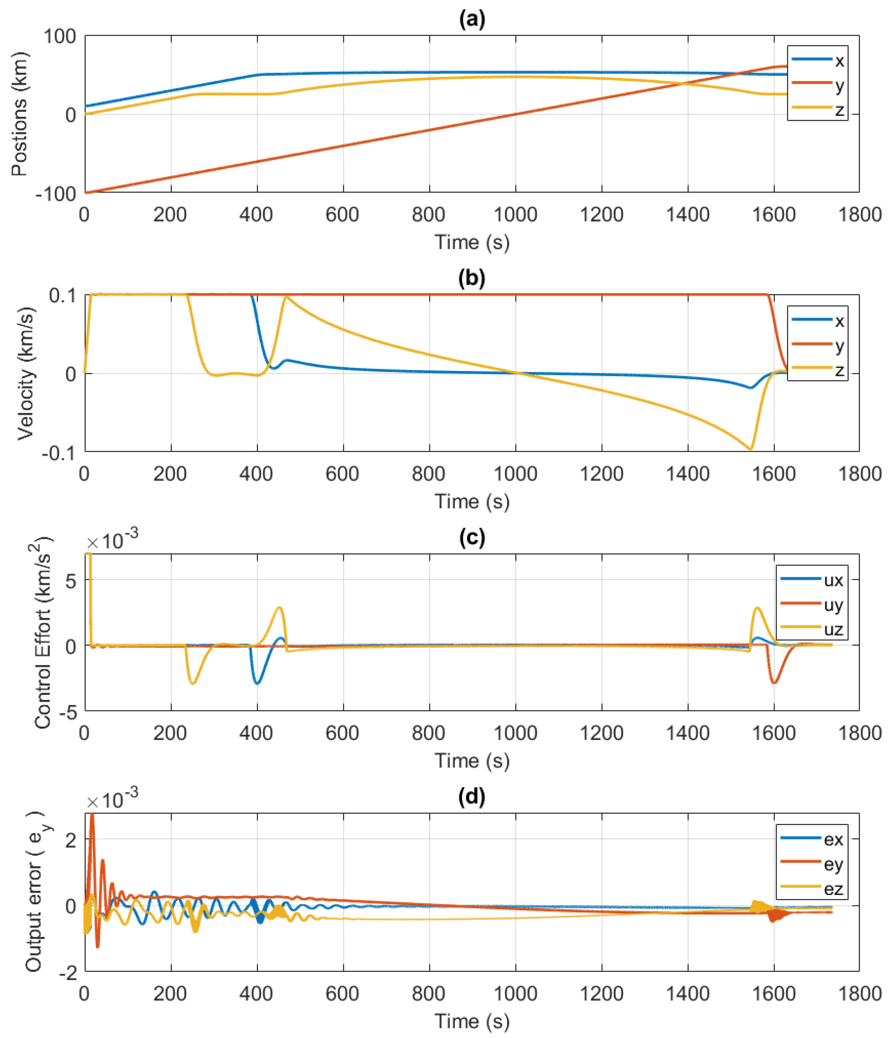
Figure 6d. The position and velocities are given in
Figure 6a,b, respectively.
It can be seen that the positions do not converge to the desired position and the velocities do not converge to zero. The control effort from the feed-forward MPC is shown in
Figure 6c. It can also be noted that the ellipsoidal constraint for obstacle avoidance is not met, and the spacecraft eventually becomes located inside the constraint ellipsoid (see
Figure 7).
4.2. Case 2: Adaptive Control
In this section, the results for feedback adaptive control are presented. As the adaptive control is an output feedback trajectory tracking control, the trajectories generated from NMPC are fed into the adaptive control for tracking. It should be noted that only the feedback adaptive control from Equation (
14) is implemented. This is in order to show that even though adaptive control is able to successfully track the desired trajectories, the results can be further improved by adding the feed-forward control.
It can be seen from
Figure 8 that the adaptive control is able to successfully track the desired trajectory generated from the NMPC and converge to the final desired position. This shows the robustness of the adaptive control with respect to the irregular and unknown gravitational field of the asteroid Kleopatra. However, since the adaptive control gains are initialized with zero initial conditions, there is signification overshoot in the control effort before the gain adapts to the error between the desired and the actual output. This overshoot and chatter is corrected using the feed-forward controller as shown in a later section.
The position and velocities are shown in
Figure 9a,b. The positions successfully converge to the desired final position and the velocities converge to zero. The adaptive control effort can be seen in
Figure 9c. The output error can be seen in
Figure 9d. The output error is far less (see
Table 4) than in the previous case, which shows that the adaptive control is able to track the trajectories in the presence of disturbances.
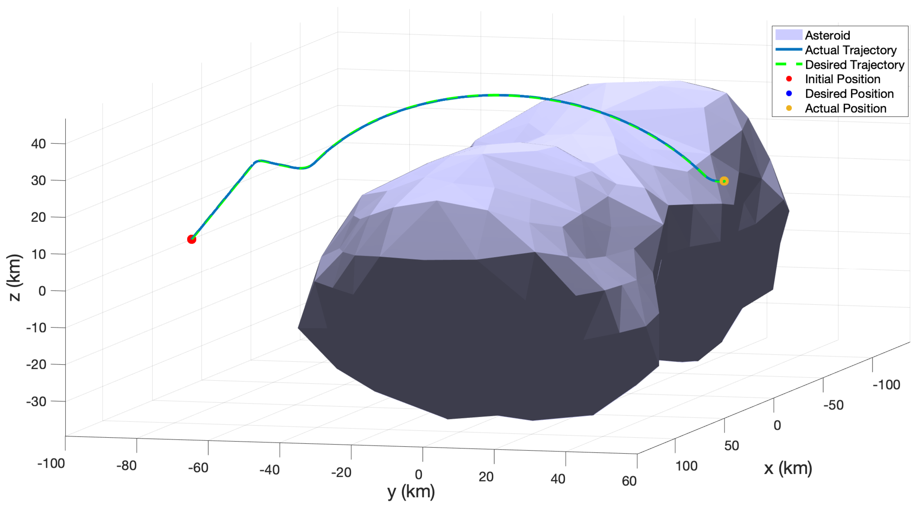
4.3. Case 3: DAMPC Implementation
In this section, the simulation and results for the combined control are presented, i.e., direct–adaptive model predictive control (DAMPC). As mentioned before, DAMPC is a combination of adaptive control and MPC, where the adaptive control is the feedback control and the NMPC is the feed-forward control, as shown in Equation (
13).
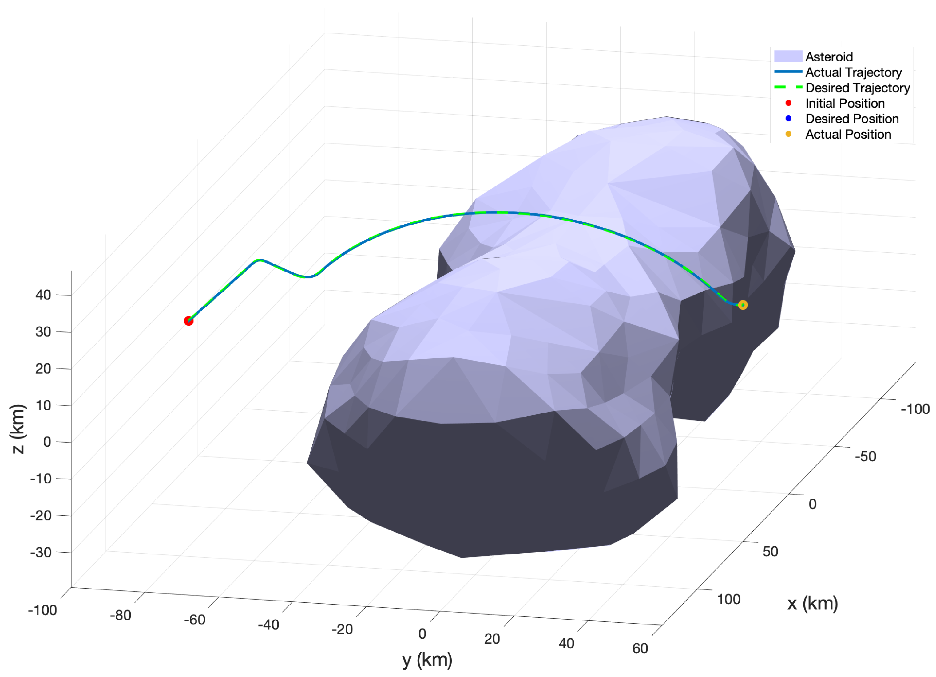
The NMPC feed-forward control values are similar to those used in Case 1. The actual and desired trajectories can be seen in
Figure 10. It can be seen that the DAMPC is able to track the trajectories successfully.
The tracking performance of DAMPC is better than that of the adaptive control, as shown in
Figure 11d. This is due to the fact that DAMPC is able to excite the system with non-zero control effort, unlike the adaptive control system. This prevents overshooting and chatter in the control system. This effect can be seen in
Figure 11c and compared to the case where only adaptive control was implemented (see
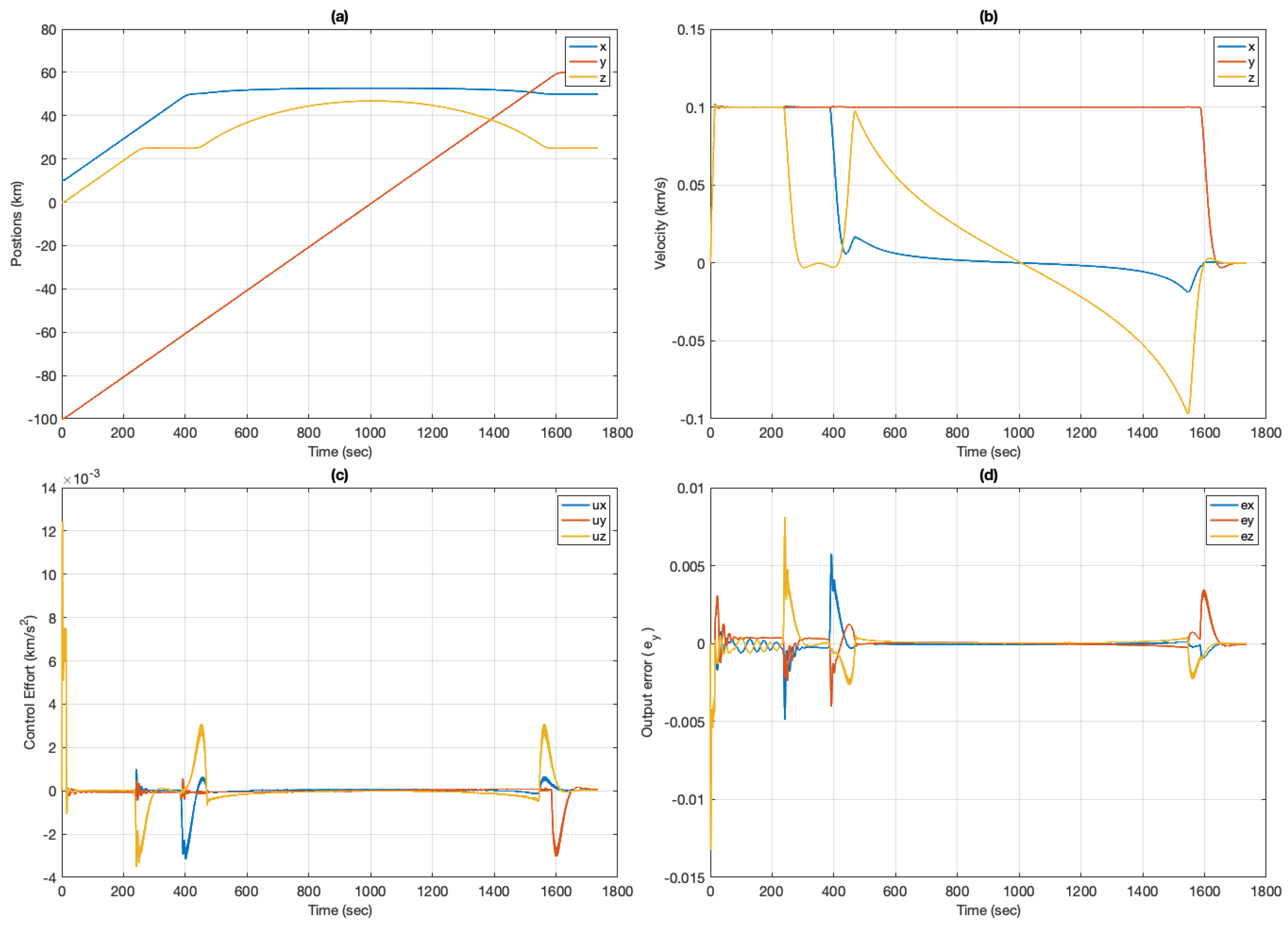
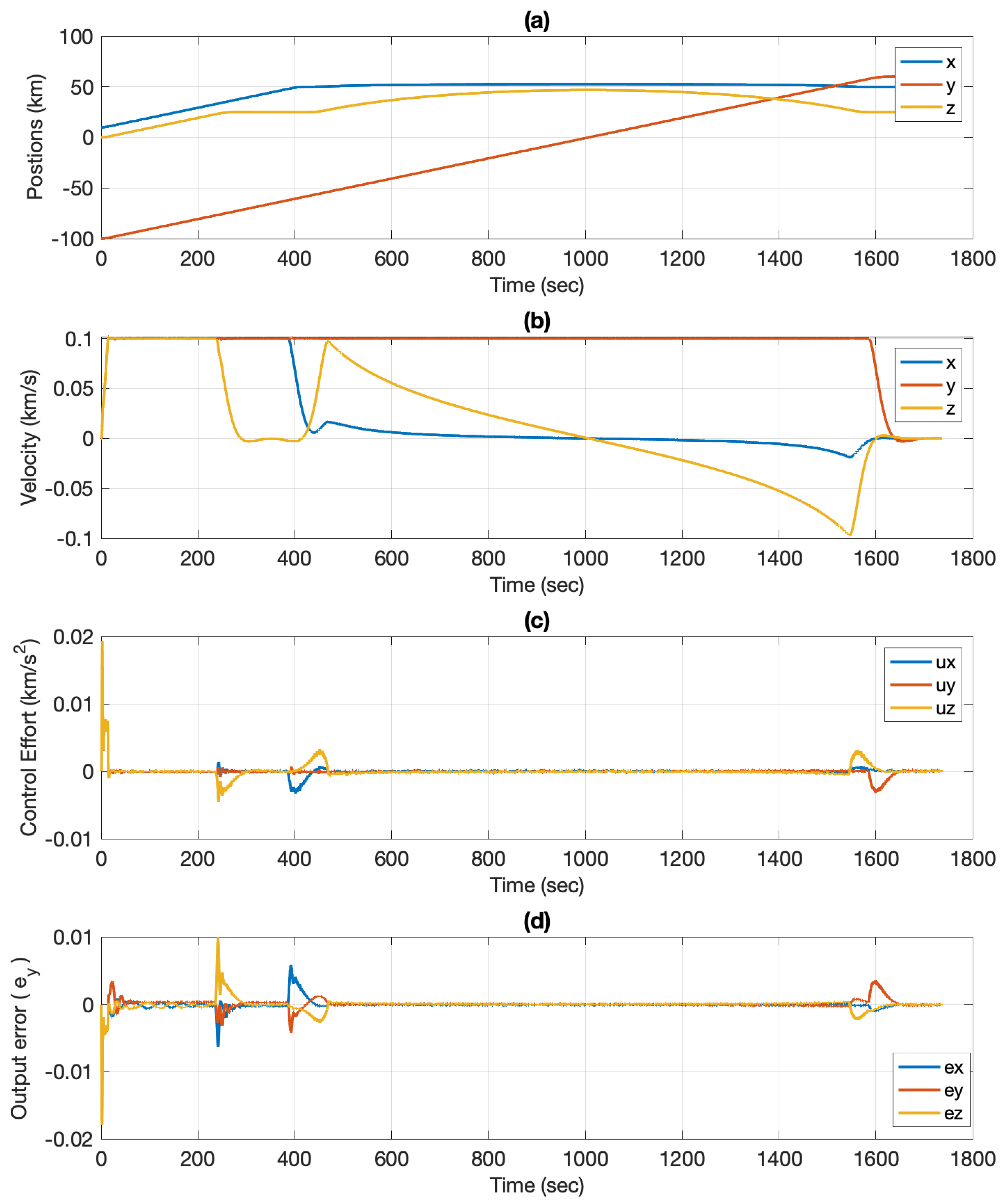
Figure 8). The position and velocities are shown in
Figure 11a,b. It can be seen that the position and velocities converge to the desired values. It should be noted that constraining the velocity helps to keep the control effort low. Increasing the velocity limit requires more control effort or increases the duration of the mission, which requires more on-board fuel. The output error (
) is shown in
Figure 11d and is significantly less than in the adaptive control case, thus demonstrating the improved performance over the adaptive control.
4.4. Case 4: Effects of Unknown Noise
In this section, the effect of noise on DAMPC and adaptive control is compared and the results presented. It was found that DAMPC offers a better tracking performance in the presence of noise and a reduced chatter in the control effort, compared to the case where only the adaptive control is implemented. A random Gaussian noise of
was added to the system given in Equation (
1) such that the system could be described as follows:
The magnitude of the Gaussian noise () was taken to be one order higher than the gravity, to further test the robustness of the control system to unknown noise.
Figure 12 shows the plots for the case where only the adaptive controller is implemented with noise and
Figure 13 shows the corresponding plots for DAMPC. It can be seen from the figures that DAMPC is able to handle the noise better than adaptive control, in terms of the output error and control effort.
Figure 12e and
Figure 13e show the increased control effort, and it can be seen that the control effort and chatter for DAMPC are less than for the adaptive control.
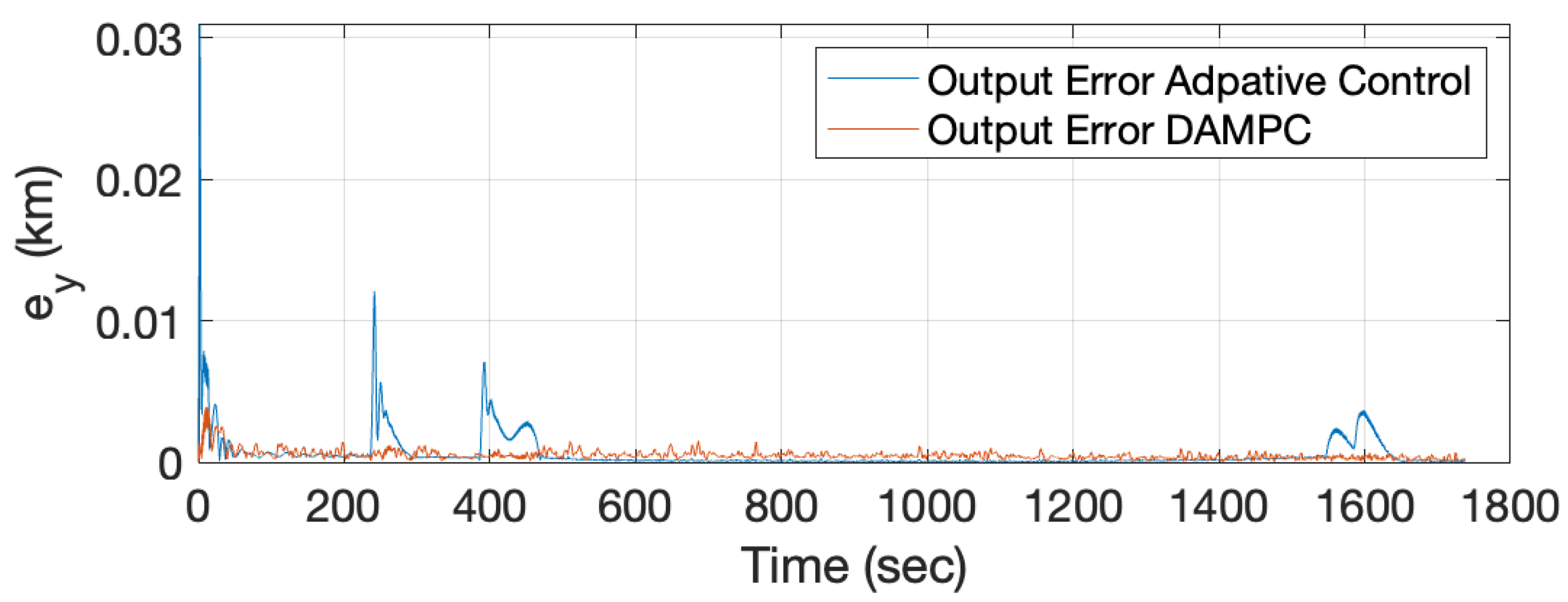
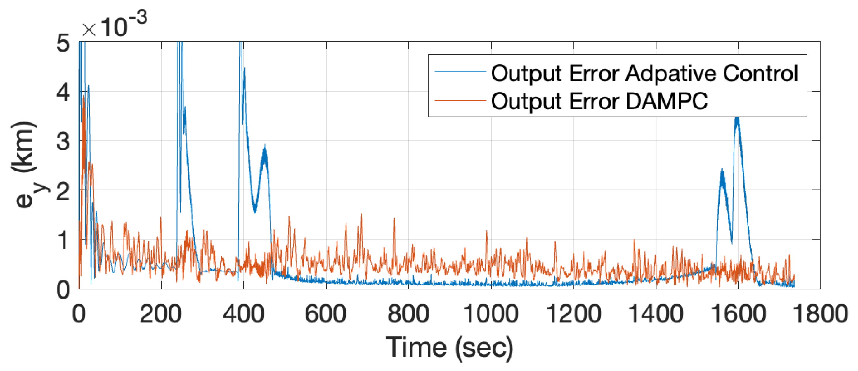
Figure 14 shows the comparison between the output errors for a noisy system with adaptive control and DAMPC. It can be seen that although the adaptive control is able to handle disturbances, the DAMPC control is also able to avoid overshoot in the output error and keep the overall output error normalized. A zoomed-in plot is shown in
Figure 15.
It should be noted that the performance of NMPC is also dependent on the type of numerical solver used and its various parameters. In this work, CasADi [
24] was used as a solver. However, several other types of solvers and methodologies can be implemented, and more research needs to be done in order to identify the best solver. It should also be noted that DAMPC is agnostic to the type of optimal control technique applied. Therefore, for a linear system, a linear quadratic regular (LQR) or linear quadratic tracker can also be implemented.
4.5. Case 4: Other Effects
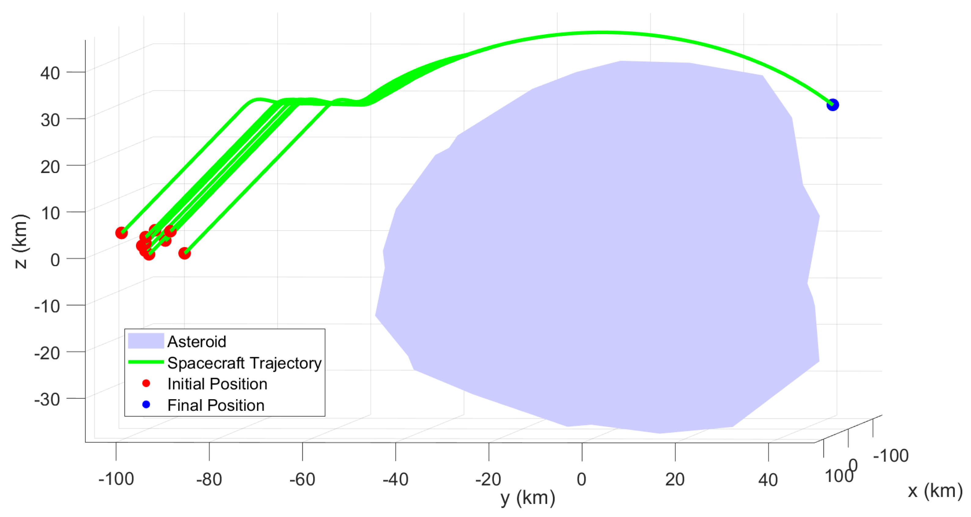
In this section, we discuss other conditions that can significantly affect the performance of the controller. In
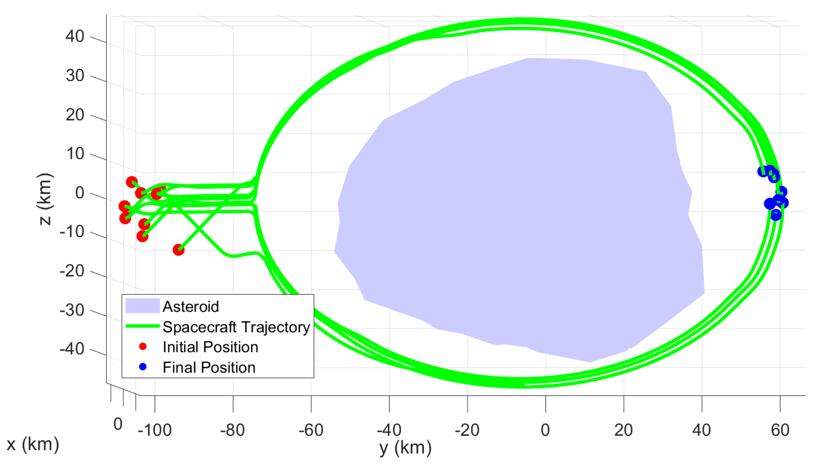
Figure 16, we show the effects of varying the initial conditions. The initial conditions are generated using a random Gaussian distribution, and the DAMPC controller is not manually tuned to accommodate to these new initial conditions. It can be seen that the controller is able to successfully track the trajectories for these randomly generated initial conditions. To further show the robustness of the controller,
Figure 17 shows the effects of different initial and final conditions. Here, the distances to the asteroid are varied to show that the controller is able generate and track reference trajectories without re-tuning the gains.
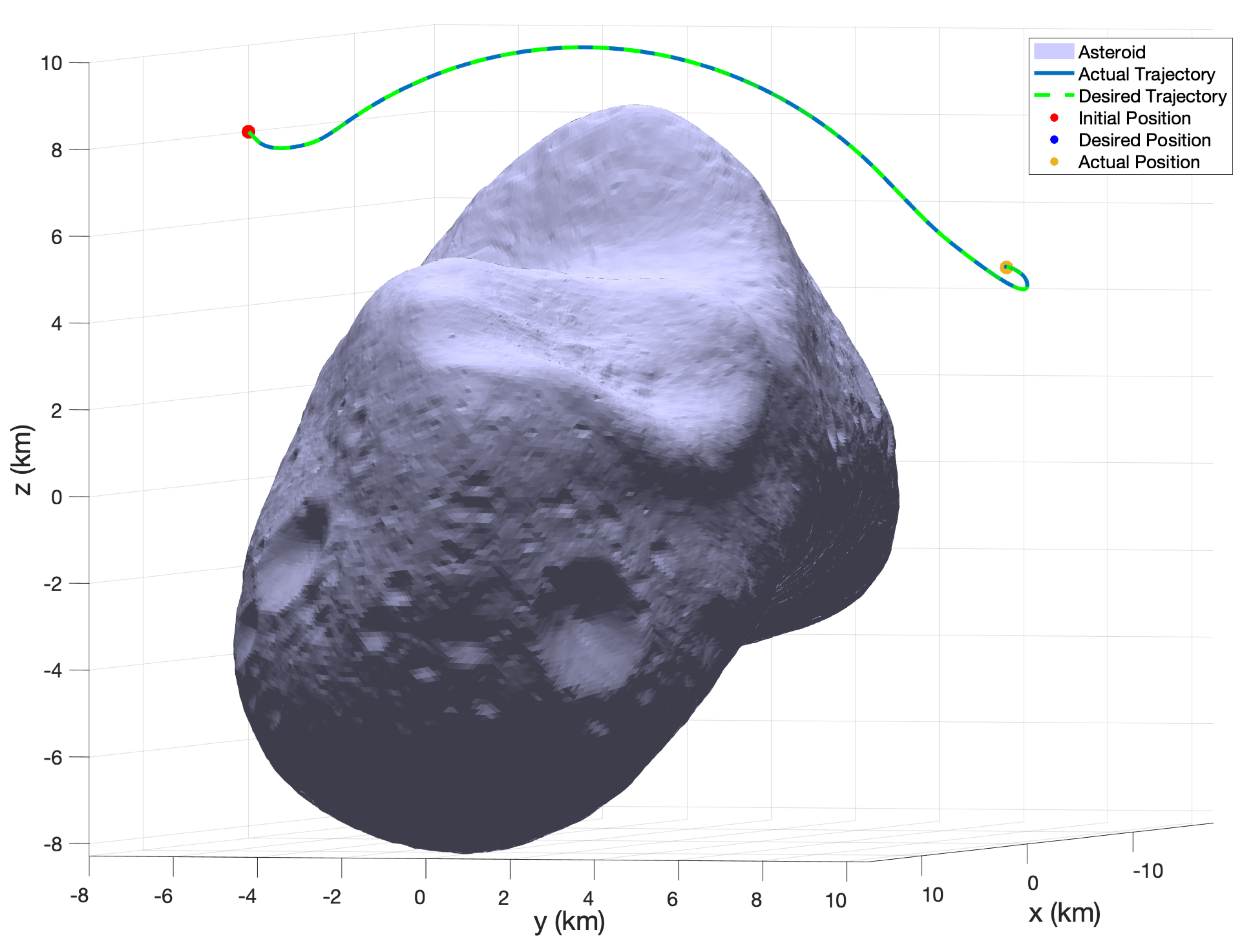
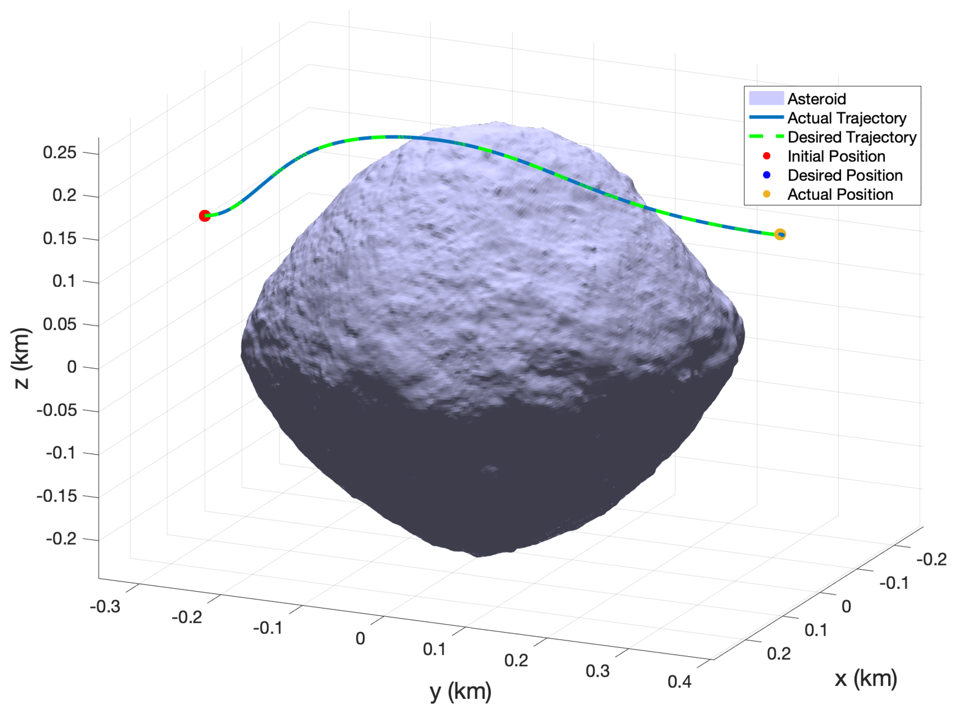
It should be noted that the gravitational field of the asteroid is difficult to estimate due to its irregular shape and density. We simulated the proposed DAMPC controller with different asteroids: Eros and Bennu. These asteroids differ greatly from each other with respect to shape, gravity and angular speeds. It can be seen from
Figure 18 and
Figure 19 that the controller is able to successfully track the trajectories. It should be noted that the controller is not manually re-tuned for either the MPC or the adaptive control. This shows that the controller is robust under varying conditions.
5. Conclusions and Future Work
In this paper, direct–adaptive model predictive control (DAMPC) was developed and applied to spacecraft control in the vicinity of an asteroid. The dynamical system was represented with a polyhedral gravity model, along with the gravity gradient force. The force due to solar radiation pressure was modeled using a flat plate model. For numerical comparison, random Gaussian noise was also added to the system to test the controller’s response.
The direct–adaptive model predictive controller was composed of a feedback controller based on simple adaptive control (SAC) theory with a robust modification and a feed-forward control based on nonlinear model predictive control. The combination produced a robust controller with the ability to generate and track sub-optimal trajectories.
The direct–adaptive model predictive controller was numerically tested for the case of the asteroid Kleopatra, for a rest-to-rest maneuver. It was shown that the controller was able to successfully generate and track reference trajectories while avoiding hitting the asteroid. Furthermore, the controller was compared with adaptive control for the system with unknown random Gaussian noise, and it was shown that DAMPC was better at handling the noise than the adaptive control.
In future work, we plan to design an algorithm to implement DAMPC for multiple moving obstacles for a multi-agent system, with real-time and on-board implementation of the model predictive controller.


