1. Introduction
With the increasing complexity of aircraft systems, the design cost to modify or introduce pipes in an existing aircraft increases. The reason for this is that aircraft systems are mostly routed in the same areas, that segregation and clearances are at their limits, that the access and installation sequences need to be considered from the beginning and that the modification of one system should not lead to a cascading change in other systems.
Aircraft systems and pipe work are impacted by several design evolutions during the life-cycle of an airplane. From the first design to the subsequent iterative incremental modifications during its service life the routing of aircraft systems has to be created, modified and adapted several times in an aircraft life to meet the latest aviation requirements and manufacturing technologies or to incorporate design improvements or corrections.
Furthermore, design trades for the overall optimization of a future aircraft must consider different architectures and locations of new equipment and pipe routing. Current pipe work is a manual process of routing the pipe through the installation area, while taking into account all clearances, manufacturing and installation requirements. All these attempts increase the non-recurring cost of every change, thus reduces the profit for the aircraft manufacturer. Aircraft manufacturer are therefore constantly looking for optimization and automation of the pipe design process. For this reason, this paper explores the application of graph-based design languages for design automation in the specific case of piping design automation.
However, the task of designing the necessary pipework (i.e., the so-called “piping”) of hydraulic system components inside an aircraft is not an isolated design effort with constant interfaces or constant pre- and post-conditions, but is embedded in a complex systems engineering and design process instead with constantly changing boundary conditions and goals. It is therefore worthwhile to shortly analyze the overall design process in order to understand both the position of piping in the current aircraft design hierarchy and sequence, as well as the mutual implications of physical system architecture design on piping and of piping on physical systems architecting vice versa.
1.1. Graph-Based Design Languages
Graph-based design languages are inspired by natural, human languages, in which the vocabulary and rules form a grammar. The term “design language”means that every sentence built with the available vocabulary and allowed by the grammar is a valid expression of a design. The term “graph-based”means that each node in a graph is used to represent a requirement, a product function, a solution principle, a component or an assembly, or any other arbitrary engineering concept one may encounter in or along the product life-cycle. The graphical representation of design languages is based on the Unified Modeling Language (UML), an international standardized data format in order to avoid vendor lock-in and capable of self-defined extensions.
A design language encodes the complete knowledge of the design product and its associated design processes in form of a graph-based, machine-readable and machine-executable form and is translated by a design compiler (the design compiler used to compile graph-based design languages in this paper is the Design Compiler 43
® [
1]). The key components of a graph-based design language are the vocabulary, the rules and the production system. In case graph-based design languages are implemented using the UML, the vocabulary is represented in form of a UML class diagram, the rules are represented as Model-to-Model (M2M) or Model-to-Text (M2T) transformations. The production system is represented in form of an UML activity diagram. The result of the compilation of a graph-based design language in a design compiler is the design graph, an UML instance diagram. This is later mapped into different domain-specific languages (DSLs) by dedicated design compiler software plug-ins for further processing, typically for visualisation purposes such a CAD-model in an external CAD-kernel or for simulation purposes such as a finite element model (FEM) simulation in an external FEM solver.
According to the Engineering as a Service (EaaS) paradigm, an engineering design activity such as the automated piping in arbitrary complex 3D geometries which will be described in this work, is encoded as an executable engineering service in a design compiler serving as an integration platform. The design compiler platform offers inbuilt digital continuity and consistency for all engineering data due to the generation of all engineering models from a single source. As known from any other formal programming language compilation run in a compiler for that language, a single design language (or several design languages combined together) can therefore be considered as one single source of truth which is compiled into different domain-specific models (CAD, FEM, …) which are therefore automatically consistent to each other. The 3D piping algorithms are built into a design language as an executable engineering service for later reuse in a multitude of design contexts (aerospace, automotive, marine, etc.).
For this reason, the main focus of this paper is on 3D piping in arbitrary complex geometries only and the design language approach sets for the purpose of this paper just the framework of building software hulls (i.e., interfaces) around the algorithms to make them later reusable in automated process chains. The details of the 3D piping algorithms and an in-depth analysis of their performance will therefore be described in great detail later in this work. It is the algorithm which matters in theory and not the implementation, despite the fact that a thoughtful implementation will make the difference in both runtime and memory requirements in practice.
For any further explanations and properties of graph-based design languages and the design compiler approach, the reader is referred to the already quite extensive body of literature about graph-based design languages [
2,
3,
4,
5]. More specifically, any reader interested in a comparison of graph-based design languages with other related graph transformation approaches is referred to a most recent survey paper which reviews the commonalities and differences of graph transformation approaches [
6] and which represents a follow-up of a previous survey paper [
7]. Similarly, a further performance comparison of the design language approach with other model-based transformation and mapping concepts [
8,
9,
10] is intentionally not dealt with in this paper.
1.2. The V-Model of Model-Based Systems Engineering
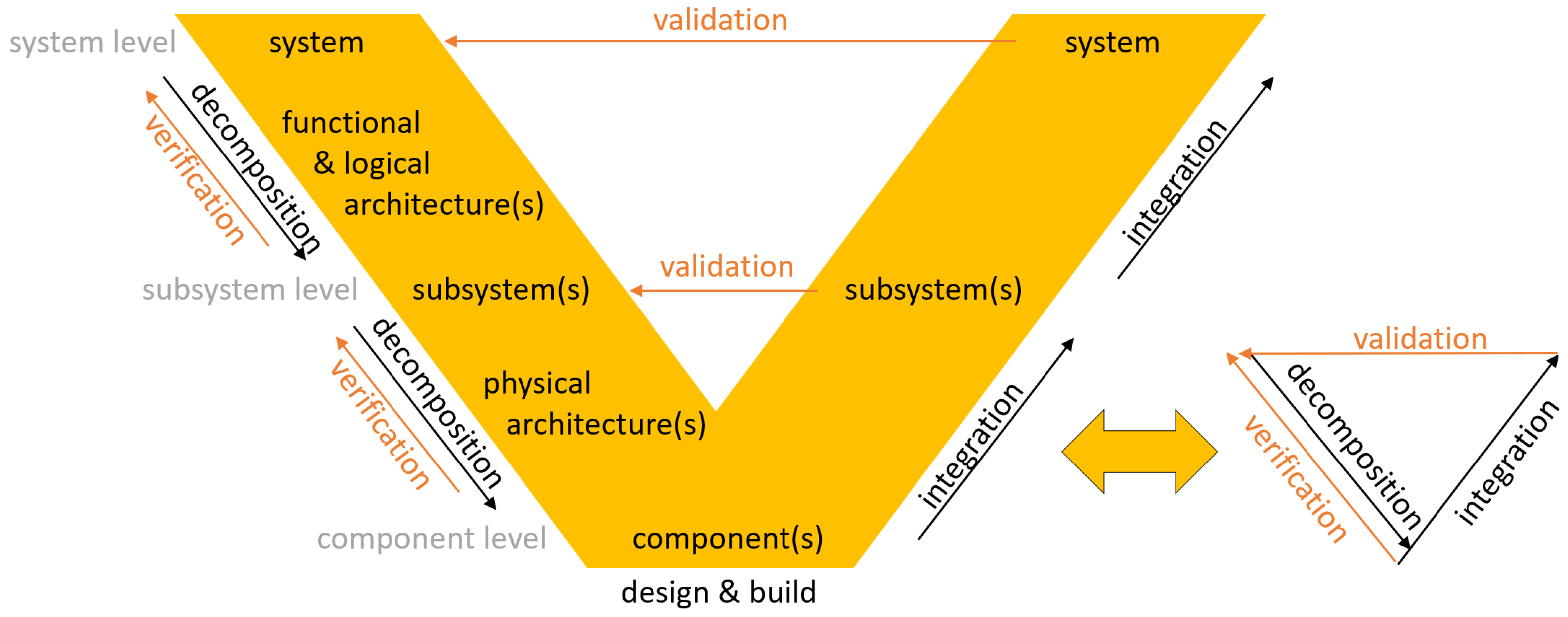
The V-model in
Figure 1 illustrates the clearly structured approach of model-based systems engineering (MBSE) in the development of complex systems such as aircrafts: Starting from requirements (due to the central role of requirements for product shape, behavior and usage definition, one therefore often speaks of requirements engineering and, when in the verification analysis, only that has been designed and built which is specified in the requirements, it is also referred to as requirements-driven engineering), these requirements are decomposed and mapped in several decomposition steps into a functional architecture, then mapped onto a logical architecture and finally mapped into a physical architecture. On the left side of the V-model it is checked by verification measures whether the decomposition, i.e., the mapping of the requirements from the respective level to the respective subordinate level, is correct. Accordingly on the right-hand side of the V-Model, validation measures are used during integration, i.e., during the process of system assembly it is checked whether the components, subsystems and the overall assembled system meet the requirements which is checked by tests associated with each requirement.
Piping furthermore depends heavily on the previous placement (the so-called “packing”) of the hydraulic system components inside the aircraft, since any change of a component’s position or orientation affects the start- and endpoints the pipe connection and their spacial orientation. Both problems of packing and piping [
11,
12] are known to fall mathematically speaking into the class of so-called “NP-hard problems”, for which no exact algorithmic solution in polynomial time-complexity is known [
13]. This means that the development and advantageous use of problem-specific search heuristics or problem-independent meta-heuristics to circumvent and overcome this existing hard theoretical bottleneck is therefore mandatory. One often chosen way of mastering this theoretical obstacle is to use an algorithm which only approximates the solution and which is therefore capable to sacrifice optimality for speed (algorithms such as the simulated annealing algorithm [
14] in
Section 4.2 are known to return solutions up to only several percent away from the true optimal solution while consuming only a fraction of the original polynomial runtime which is, seen the circumstances, considered as an acceptable runtime behavior).
In a complete design scenario, the design process would start on the top left of the V-model in
Figure 1 with the requirements for the hydraulic systems, goes on with a functional decomposition yielding the functional architecture, and then move on to the development of a schematic of the hydraulic system as the logical architecture. Then the hydraulic system components would need to be physically allocated, which results in the so-called
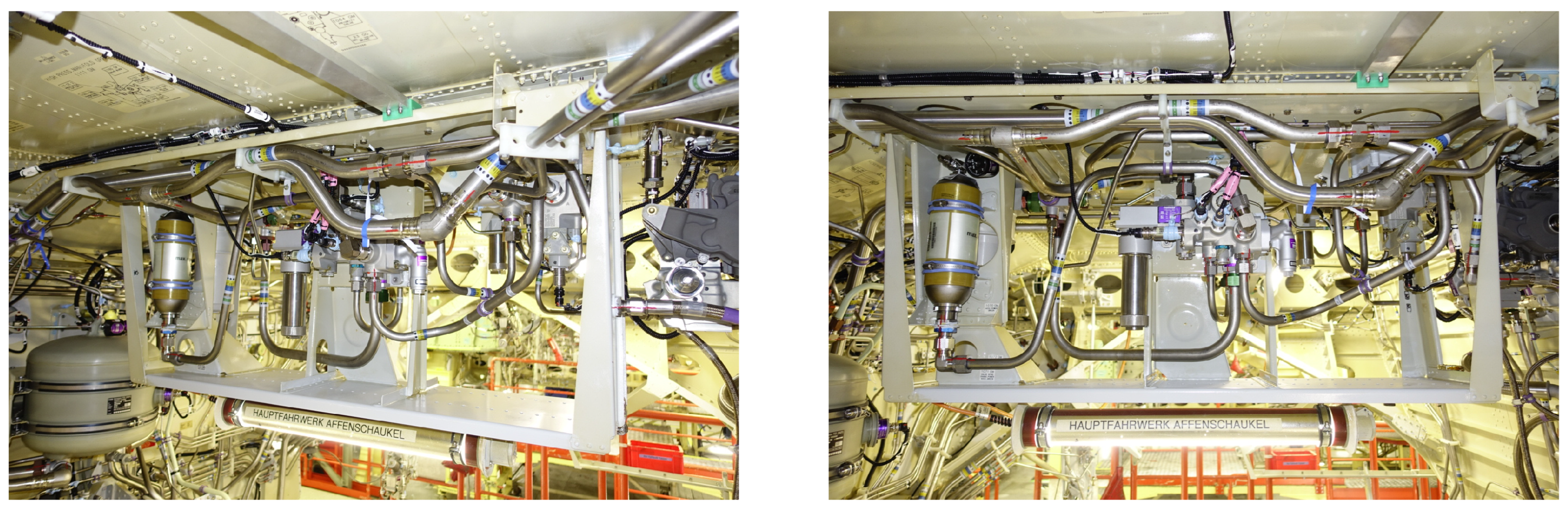
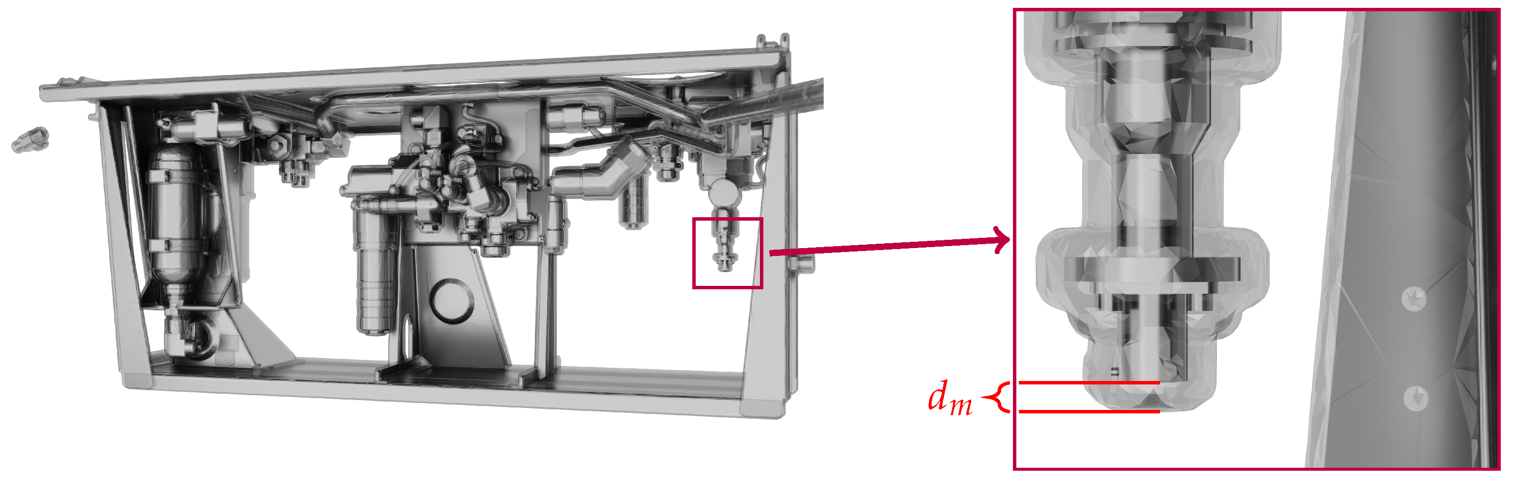
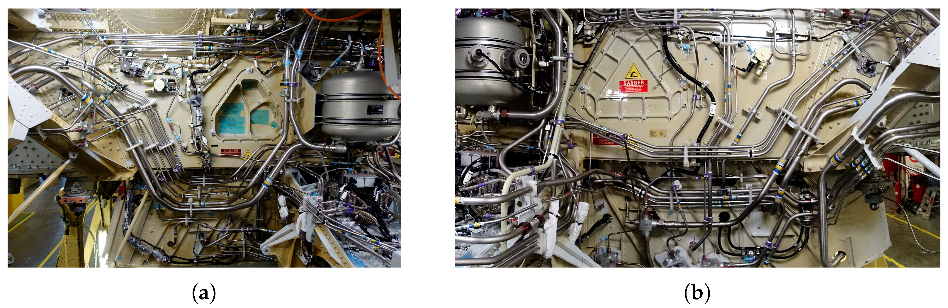
package. In the current paper, both the functional and the logical architecture as well as the package are already predetermined, since all these data are adopted from the shown industrial use-case of a A320 series solution. The series solution of the pipe work in an Airbus A320 mounting rack can be seen in
Figure 2 as an example of the typical complexity in an aircraft pipe network installation. Therefore, the task of finding automatically (i.e., through a “1-click solution” by the press of a button) a set of feasible piping connections in an arbitrary complex 3D geometry remains and is described in the following sections of the paper.
The future vision of an automated MBSE includes therefore a machine-executable V-Model [
5] which stands for the automated execution of a workflow [
15] of fully interconnected and interoperable
engineering as a service (EaaS) software modules such as automated packing and piping. The piping automation is thus just a small portion of a larger research effort [
16] to achieve an intelligent design automation [
3] using design languages translated by a design compiler into executable models [
17].
Since the design decision making on the packing, the logical and the functional architecture are located upstream in the design process, these decisions form the future outer optimization loops where the functional architecture sets the boundary for the logical architecture and the logical architecture sets the boundary conditions for the packing. As the most inner nucleus of these nested optimization loops, the automated 3D piping described in this paper generates feasible connections and refers in this respect to the most inner validation and verification patterns in the V-model on the right hand side in
Figure 1. As said in the beginning of this paragraph, that if the scope of the work would cover also the more upstream design decisions of packing, logical and functional architecture definition, the consequences of these decisions could be investigated by an exploration of the design by looping through the alternatives.
1.3. Manufacturing Technology Influence
The pipes generated by the proposed algorithm should be able to be manufactured with the rotary draw bending process for bending machines described in VDI 3430 [
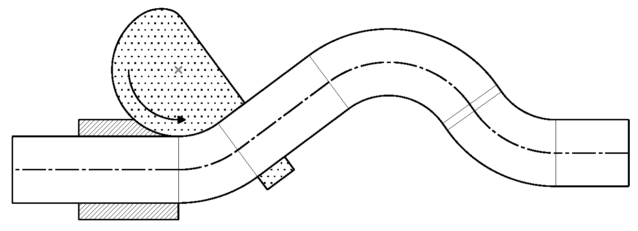
18]. In this process, only bends with a fixed bending radius can be bend. The bending angle can vary within a certain range determined by the bending machine. Between two bends, a straight pipe with a minimum length has to be placed. This leads to an alternating order of straights and bends. As a result of the construction of the bending machine, a minimal distance between the bends must be established if the bends should be bend independently. Furthermore, a limited, machine depending number of bending claws can be used to manufacture two bends with a smaller straight distance in between.
In
Figure 3, the process is illustrated. The pipe is drawn along the fixed dies (shown in a dense hatching) and is bend around the rotating die (shown in a dotted hatching). As a result of this the bending radius is constant for a specific pipe as mentioned before because every bend is bend around the same die. If the distance between two bends is too short to retain the pipe by the rotating dies the pattern of the pipe needs to be milled into a specific bending claw.
1.4. Design Process Influence
Both the start- and the end-points with their respective directions (i.e., the tangents), the pipe diameter and the properties of the intended bending machine must be known in advance. In addition, minimal distances of the pipes to certain obstacles and to each other that must be adhered to, can be set. Furthermore, a user is able to affect the piping algorithm by modifying the weighting of the different evaluation factors which will be described in more detail in
Section 4.1.
2. Related Work and Research Gap
In this section, different approaches by other researchers are discussed. The discussion is arranged from the approaches close to the manual design, like a knowledge based expert system, to multi-objective approaches with three-dimensional obstacles. Subsequently the drawbacks of the discussed approaches are worked out and the research gap, which this paper focuses on, is described.
2.1. Related Work
In the past, quite a few different approaches to solve routing problems have been investigated and published. These approaches differ in the multitude of the recognized objectives, the complexity of the obstacles which can be taken into account and the level of detail mastered in the routing process.
Simplified approaches. The approach which is most related to the manual design process is a knowledge based expert system. In a system like this empirical knowledge and documented design knowledge is used. The system proposed by Kang et al., 1999 [
19] is an example. A system without the need of empirical knowledge is proposed by Niu et al., 2016 [
20]. The installation space is discretized with a regular grid. The obstacles are considered by cell blocking and the pipe path is searched by a NSGA-II algorithm on the grid. As a result of this the pipe can only be bend with
bends. Another approach, which was proposed by Qu et al., 2018 [
21], is based on an octree grid combined with an max-min ant system optimization algorithm. The obstacles are approximated by divided, deactivated grid cells and the pipe path is searched on the grid. Moreover a graph based approach is proposed by Kim et al., 2021 [
22]. The graph is created with its nodes and edges and the shortest path on the graph is searched. The, manually simplified, obstacles are taken into account by deactivating the intersecting graph edges. This leads to short runtimes (in the order of minutes) but no other objectives than the length is taken into account. In addition, the diameter of the pipes is neglected.
Broader approaches. Thantulage 2009 [
23] proposes in his dissertation a method based on regular and random grids for pipes with different bending angles. The paths are optimized by an pareto-based general-purpose ant colony algorithm (PSACO) developed in the thesis. Thantulage facilitates the collision detection library RAPID which can process obstacles of any shape. Liu and Jiao 2018 [
24] extend an existing pipe routing algorithm based on NSGA-II with a vibration analysis. This algorithm is able to generate pipes with non-discrete bend angles. Furthermore the algorithm does not search on a grid, so the pipe path is not limited to a predefined grid. A grid based method for the generation of different pipes, which could intersect each other, is proposed by Wang et al., 2006 [
25]. The method is based on an unmentioned genetic algorithm. Another suggested method is to use a system which is intentionally designed for the motion planing of a robot. In his dissertation Lee 2014 [
26] uses the Motion Planning Kit developed by the Stanford AI Laboratory. In a post processing step the computed trajectory is smoothed to get a pipe path.
Sophisticated multi-objective approaches. An approach for arbitrary pipes is given by Szykman and Cagan 1996 [
27]. They suggest an approach for non-orthogonal routes which are optimized by a simulated annealing algorithm. A trade-off between the length of the pipe and the number of bends is shown. The path is not limited to a grid, but the obstacles can only have the shape of a cuboid or a cylinder. Another limitation is that the segments of the pipes are assumed as one dimensional and the bends are not rounded. A combined optimization of pipes and the corresponding clamp positions is described by Liu et al., 2021 [
28]. The optimization is done by an Improved Multiobjective Ant Lion Optimizer with the objectives pipe length and flow resistance, supplementary six constraints such as a maximum bend angle and a minimum length between two bends have to be considered. The algorithm takes convex hulls of obstacles into account but the design space is limited to the mathematically described surface of an aero-engine. A clash avoidance of the pipes between each other is not described. Some authors of Liu et al., 2021 [
28] are also authors of Yuan et al., 2021 [
29], which propose a method divided into three steps: pipe grouping and sequencing, multiple pipe layout optimization and pipe parallelization optimization. The routing problem is reduced to a 2D task on a cylindrical shaped aero-engine surface. The obstacles on the surface are modeled by a grid in which the weights of the grid cells determine if the cell is forbidden for a pipe or not. These reductions lead to small runtimes in the order of minutes. Additionally to the parallelism of the pipes the objectives pipe length, pressure loss, space occupancy and obstacle avoidance are considered.
2.2. Drawbacks and Research Gap
The shown related works have in common, that the solutions have only been used for problems with a relatively small number of pipes and/or without arbitrary complex obstacle geometries (in 3D) and/or without taking the manufacturing constraints related to the bending machine into account.
Drawbacks of grid-based approaches. Pure grid- or cell-based algorithms have an inherent resolution limitation as a result of finite computational resources, on the other hand a high resolution is necessary to be able to route through, compared to the overall size, small holes. Moreover arbitrary bend angle, which are necessary to get solutions in arbitrary complex installation spaces, also need a high resolution of the grid or cells because only discrete angles can be produced if the pipe has to follow grid points. Algorithms where the bend positions are not limited to an grid offer the possibility to overcome these difficulties.
Research gap. For an industrial application, like the pipe work in an Airbus A320 main landing gear bay, dozens of pipes, which can interact with each other and need to be able to be manufactured on a bending machine, located in an arbitrary complex installation space need to be mastered by an algorithm. Additionally the runtime and computational demand should not be too extensive otherwise it is not practical to use an algorithm in an industrial environment. This means that the runtimes should be within hours or days so that different variants can be generated and evaluated by an engineer within a week. Such requirements and the consequential challenges are not limited to the aerospace industry, Kim et al., 2021 [
22] describe these also for the automotive industry using the example of the Hyundai Motor Company. In summary, it can be said that this paper focuses on the research gap to propose a multi-objective pipe routing algorithm which can solve a 3D routing problem consisting the interaction of pipes with different pipe types (diameter, minimal distances, etc.) in arbitrary complex 3D installation spaces in a runtime short enough to be used in an industrial environment.
3. Pipe Routing Process: Overview and Preprocessing
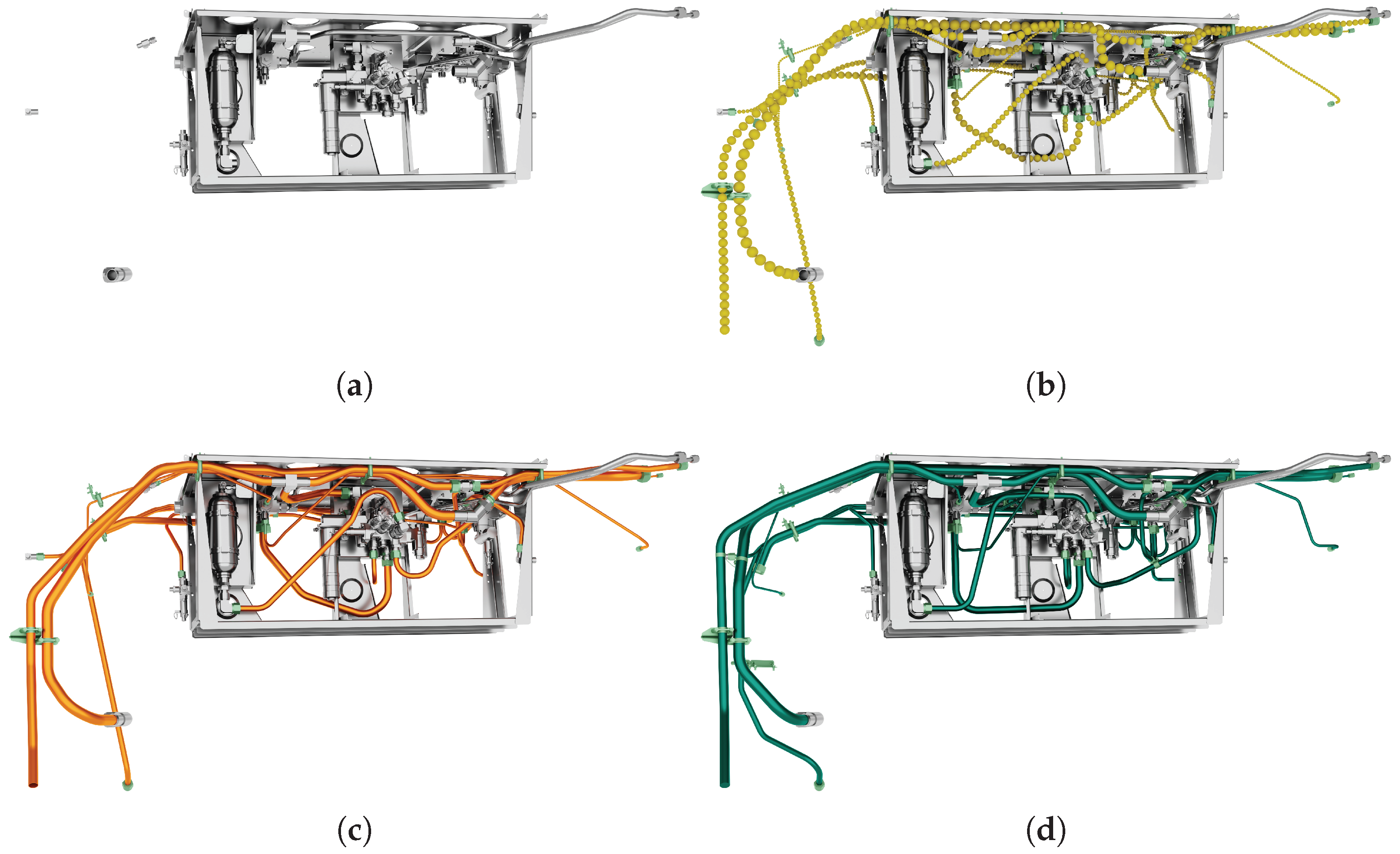
In
Figure 4 an overview of the overall process is shown. The presented geometry is subsequently used to demonstrate the process, which will be described in the following sections. At first a preparation of the inputs is done (
Figure 4a), after that paths through the installation space are found as a first approximation (
Figure 4b) and after that the optimization of the pipes is done (
Figure 4c). After the description of the piping process the automatically generated solution is compared to the manually designed solution (
Figure 4d).
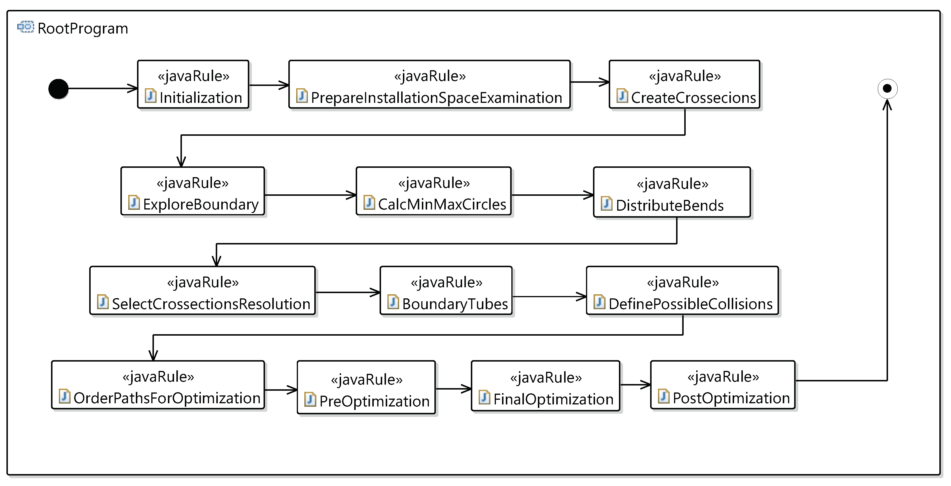
The root program of the design language is shown in
Figure 5. It consists of several subordinated design languages in which the pipes are generated and optimized based on the paths through the installation space. This illustrates the fact that many steps are necessary to create automated generated pipes.
As it is described in
Section 1.1, this design language is compiled and executed by a design compiler. A part of the corresponding class diagram is shown later. The rules, which are shown in the root program, define how the pipe design process is carried out. An example, how a rule leads to modifications in the design graph, is given in
Section 3.3 together with an exemplary design graph.
3.1. Paths through the Installation Space as a First Approximation
A routing from the desired beginning to the desired end of the pipe is required. To accomplish this task an existing plugin for wire harness design [
30] is used, which is part of the industrial Design Compiler 43
® software suite [
1]. This plugin uses an A* algorithm and a collision detection to find the shortest route through an obstacle landscape under consideration of a wire diameter and a minimum bending radius. The result of the wire harness routing is shown in
Figure 4b. As this route does not consist of discrete straights and bends it can be seen as a first, but a this stage not usable, estimation of the future correct pipe path.
3.2. Boundary Exploration for Simplified Obstacle Geometry
As the dependency between the complexity of the installation space geometry and the runtime of the algorithm described in this paper should be small, a method called ‘ray tests’ to reduce the obstacle geometry to the relevant information was developed. Along the path, in equidistant distances, planes orthogonal to the path are created through the installation space. On every plane rays are shot from the point where the path cuts the plane in a regular star shape. The points, where the rays collide with the obstacle geometry, are stored. If an additional (potentially individualized) margin shall be applied, this margin is imposed on the geometry in advance to the ray tests.
The mounting rack with an applied margin is shown in
Figure 6. This ensures that the rays hit the correct, expanded geometry. The points are connected to a polygon. An illustration of this is shown in
Figure 7. The polygons are connected one after another to form a hose. In a subsequent step the number of polygons is reduced if no additional information can be gathered of these, e.g., in straight parts.
3.3. Definition of a Pipe Path
As a result of the used manufacturing technology described in
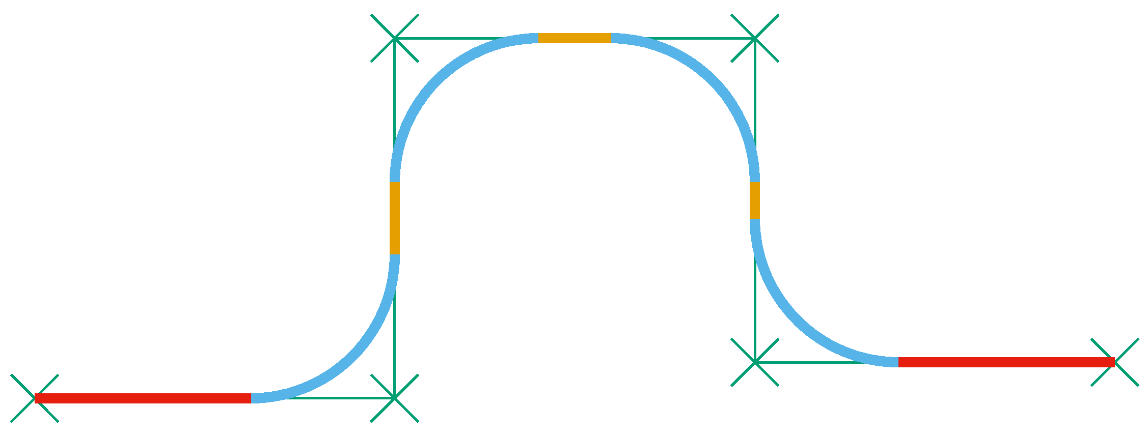
Section 1.3, the pipe path is defined as a rounded polyline with fixed arc radii. The position of the points of the polyline define the pipe path. The first and the last point of the polyline will be considered as the start- and the end-point of the pipe, respectively. If a pipe is fixed by predefined fixings, the pipe is divided into independent paths between the fixings and the paths are combined together into one single pipe definition after the optimization runs have terminated. An exemplary polyline is shown in
Figure 8.
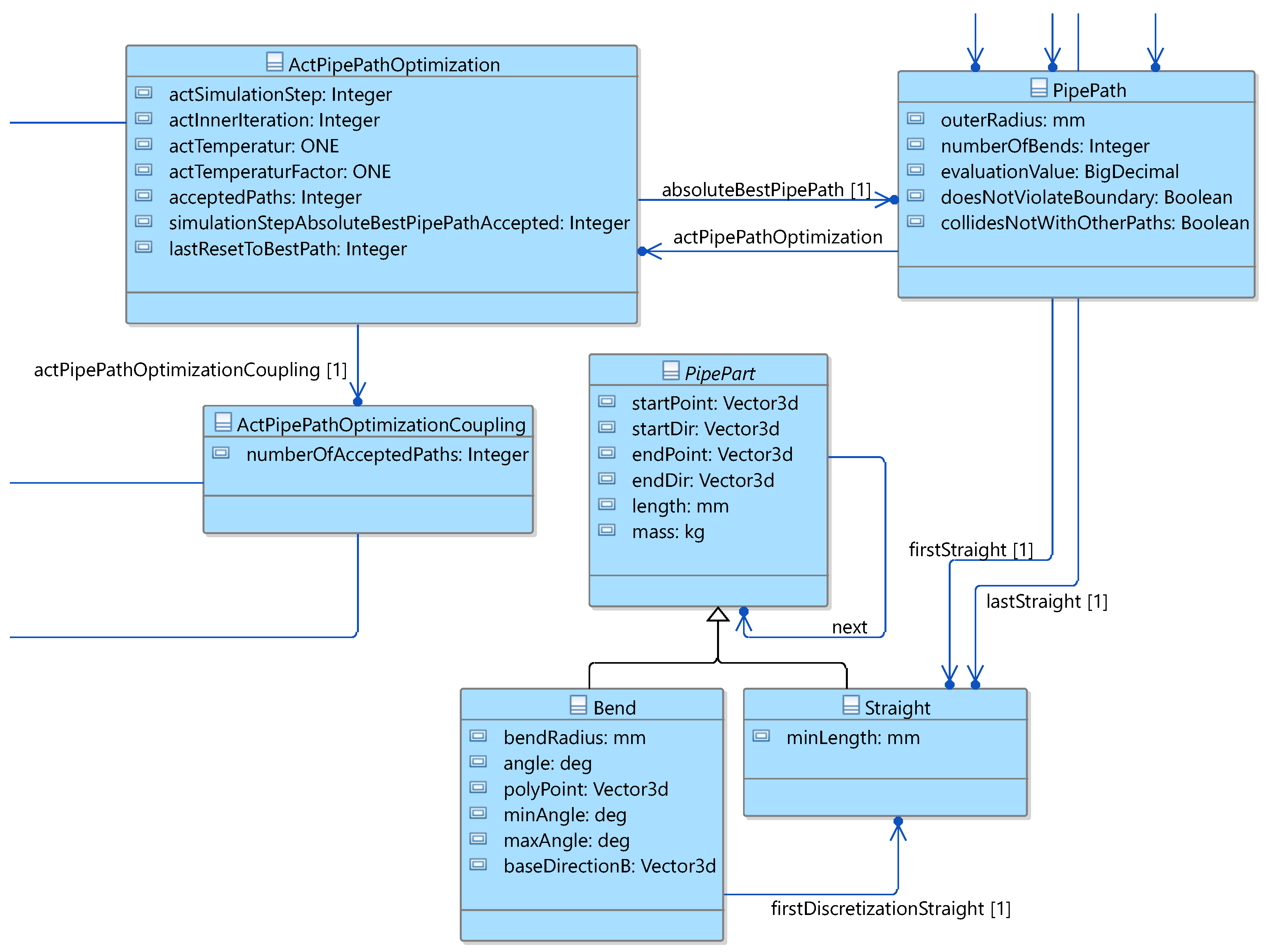
The data structure used in the design language is motivated by the structure of the pipe. In the class diagram shown in
Figure 9 the
PipePart is an abstract class. This class represents the basic properties which are necessary to define a bend or a straight. As there is a
next association from the
PipePart to itself the
PipeParts can be placed after one another. The
Bend and the
Straight inherit from the
PipePart and add the respective properties which are necessary for the complete definition. The
PipePath represents a possible solution for one specific pipe segment. As the pipe segments always begin and end with a straight only a
firstStraight and a
lastStraight association to the
Straight is necessary to assign a chain of
PipeParts to the correct
PipePath.
In the following
Listing 1, the instantiation of a
PipePath (except the first
Straight) is shown. The created instances are automatically added to the design graph by the design compiler. Therefore it is iterated over the points which define the polyline. In the iteration process
Bends and
Straights are created, linked to each other and the necessary information, for example based on the bending machine in use for the specific pipe, is put in the instances. As it can be seen in the class diagram in
Figure 9,
Bends and
Straights are
PipeParts and every
PipePart has a next link to itself, hence the
Bends and
Straights can be linked to each other. The correct start and end positions together with other geometrical values about the pipe are calculated based on this information.
Listing 1.
Instantiation of a PipePath.
Listing 1.
Instantiation of a PipePath.
PipePart pipePart = firstStraight;
for (int polyPIdx = 1; polyPIdx < polyPointsWithStartEnd.size() − 1;
polyPIdx++) {
Bend bend = Bend.create();
bend.setBendingRadius(bendingMachine.getBendingRadius());
bend.setMinAngle(bendingMachine.getMinAngle());
bend.setMaxAngle(bendingMachine.getMaxAngle());
bend.setPolyPoint(polyPointsWithStartEnd.get(polyPIdx));
pipePart.setNext(bend);
pipePart = bend;
Straight straight = Straight.create();
straight.setMinLength(bendingMachine.getMinStraightLength());
pipePart.setNext(straight);
pipePart = straight;
} |
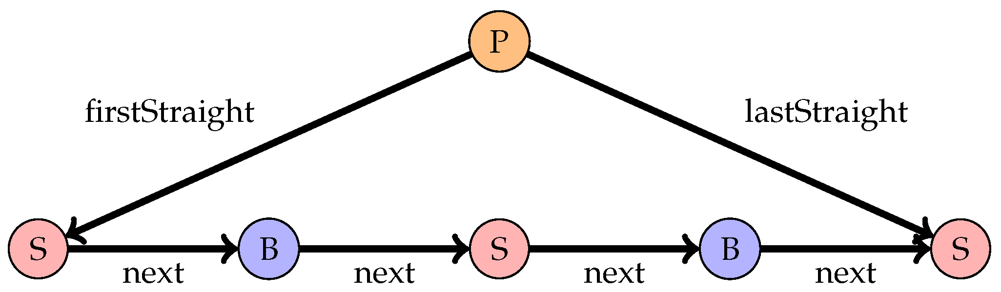
A design graph of a
PipePath is shown in
Figure 10. The instances of the
Straights (red) and
Bends (blue) are connected in an alternating order with
next links. This instances and links are created by the code shown in
Listing 1. The instance of the
PipePath (orange) is via the
firstStraight and the
lastStraight links connected to the
PathParts.
3.4. Estimation of Polyline Points
For an initial solution the positions of the points of the polyline must be estimated. All points, except the first and the last two, can be positioned in the three space dimensions. The algorithm must ensure that the distance between two following points is big enough that the bending radius can be applied and that the minimal distance between two bends required by the manufacturing technology can be fulfilled. Similarly, the first and last point are fixed and the next respectively the previous point must be on a straight line with the desired start and end tangents.
The number of polyline points is related to the number of bends. The user decides how many bends should be used at least and at most. For every number of bends in this range a pipe path must be initialized. The positions of the points for a given number of bends is estimated under the use of a path through the original installation space and the simplified installation space.
3.5. Selection of Depending Paths
The distance between the simplified obstacle geometries for each pipe (see
Section 3.2) is calculated approximately. If the distance is smaller than the allowed distance between two pipes it is possible that the pipes could intersect or be too close to each other. Therefore these pipes cannot be generated independently. As a result of this, for all depending pipe segments all combinations of estimated paths are computed. This leads to a list which pipe combinations can be optimized independently. As long as no specific generation sequence is known to yield good results this open question is answered by the comparison of the results of multiple execution sequence candidates.
4. Pipe Routing Process: Pipe Generation and Optimization
The estimated pipe paths (see
Section 3.4) fulfill the requirements imposed by the manufacturing constraints described in
Section 1.3. There exist multiple criteria, which makes a trade-off necessary. These criteria need to be weighted by a user, depending on the problem specific needs, to get one specific value which describes the overall quality of the pipe path. The pipe paths are optimized based on an evaluation function by modifying the points of the polylines which describe the pipes.
4.1. Evaluation Function and Evaluation Criteria
To get one specific value
in every iteration step
n describing the quality of the pipe path, an evaluation function is needed. A smaller value
stands for a better pipe path. The specific value
is computed by
For each evaluation criteria a value is calculated. As different criteria shall be combined, needs to be dimensionless. Referring to the method of least squares the value is raised to a specific power . Using in combination with a would lead to a better evaluation than with . In order to prevent this, the term is modified, which leads to . The result of this term can be weighted by a factor which is chosen by a user. The evaluation can be based on the following automatically determined values:
The calculation of the distance to the center line is based on the boundary exploration (see
Section 3.2). In every plane the center of a circle is calculated which has the largest radius that fits inside the boundary polygon. The circle center points are calculated with the algorithm proposed by Garcia-Castellanos and Lombardo (2007) [
31], using the euclidean distance instead of the proposed great-circle distance. The distance between the central line of the pipe and the circle center gets related to the pipe radius. For the calculation of the distance to the path through the installation space, as it is described in
Section 3.1, is used.
The selection of the weight factors depends on the given problem and the trade-off between the different criteria for the final solution. In a dense installation space it is often more promising to give the algorithm more freedom in using a higher number of bends and in extending the pipe length to find a good overall solution than to penalize this and to increase the complexity and the runtime to a great amount.
For this multi-criteria optimization problem, a single objective approach was chosen. The main reason for this is that to evaluate the distance between two pipes the pathway of both pipes must be known. This means that the evaluation of one pipe is depending on all pipes, with which pipes this pipe could be too close to each other. Due to this the pipes are optimized one after another so the already optimized pipes can be freezed and used for the following distance tests. If all pipes could be changed in the same optimization step simultaneously the search space would be too extensive for an engineering application. Therefore the best pipe must be selected, which can be done by a single objective approach. Generally speaking, a problem, which should be optimized in parallel, like the design of pipes in the same installation space, can be alternatively transformed into a sequential problem. In a sequential approach the boundary conditions can be added incremental (e.g., other pipes as obstacles). This reduces the degrees of freedom and therefore the runtime. This approach is well known as “staggered algorithms” for example in the simulation of the fluid-structure interaction. A utilization in the field of aeroelastics can be found in Farhat et al., 2000 [
32].
4.2. Simulated Annealing Optimization
The optimization algorithm must be capable to leave a local optimum to find the global optimum. Otherwise, for example two, pipes could not be moved through each other to find a better overall solution even if a clash free solution is already known. The simulated annealing algorithm proposed by Kirkpatrick et al., 1983 [
14] is able to leave local optima, therefore this algorithm was selected. For the optimization the pipes need to be modified in every step and subsequently a decision must be taken if the new solution should be accepted.
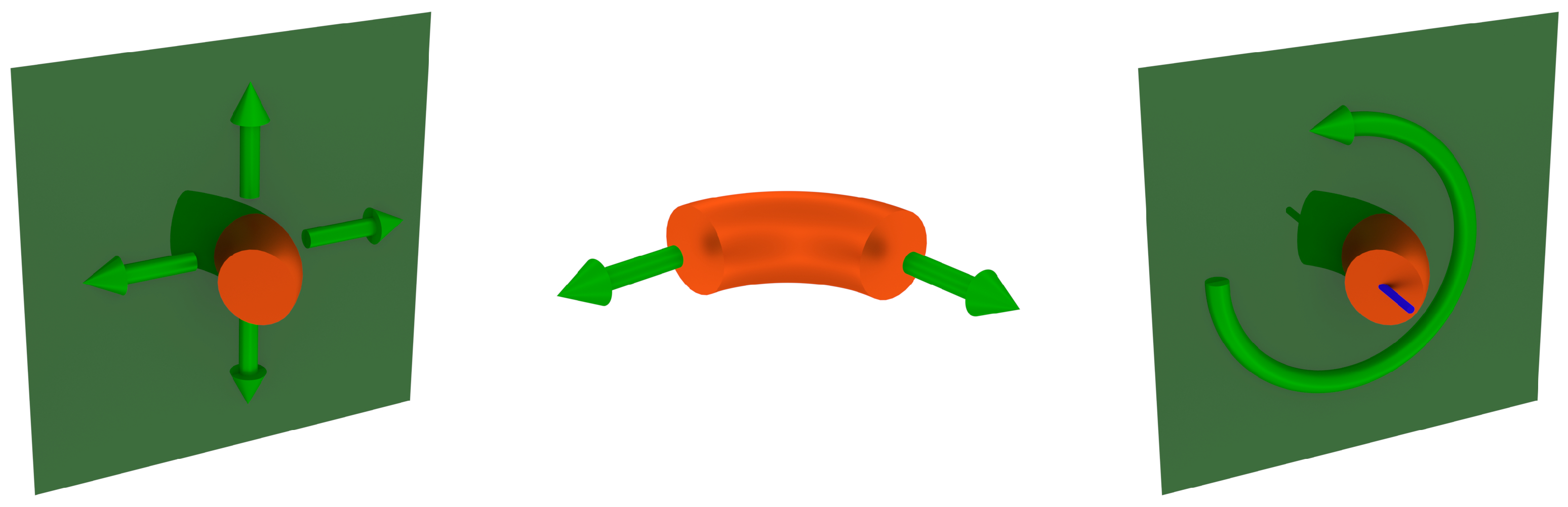
4.2.1. Generating a Modified Solution
A pipe is modified by altering the position of the points of the polyline. Additional to a random modification, more sophisticated modification schemes can be used to reach a better solution faster. A bend can, for example, be moved along its beginning and end directions, can be moved on its symmetry plane or rotated around an axis through its start and endpoint. These modification methods are illustrated in
Figure 11. The coordinates of the points
p can be
.
4.2.2. Acceptance of a Solution
The decision, if a solution is accepted, is based on the evaluation value in the actual simulation step
and on the evaluation value in the previous simulation step
. A solution will be accepted if
or
with a possibility of
As a result of this, poor solutions can also be temporarily accepted to leave a local optimum. This is a key feature of the simulated annealing algorithm. It is possible to prohibit the acceptance of a solution if a solution is known which does not collide with the obstacles and/or with the other pipes. The temperature
in the current optimization step of the simulated annealing algorithm, referring toWeyland 2008 [
33], is calculated based on an initial temperature
and a factor
k powered by the optimization step using
The factor
k is calculated based on the desired start temperature
, the desired end temperature
and the user given number of optimization steps
.
While , an acceptance of a poor result is temporarily possible. In the progress of the optimization p should be decreased. This ensures that to the end of the optimization the algorithm behaves increasingly like a hill climbing algorithm to make it certain that the final solution is the best possible solution in the specific area of the solution space.
4.3. Selection of Number of Bends and Optimization
The optimal number of bends for a pipe depends on the installation space as well as from the position of the start- and the end-point with their respective tangents, the bending radius, the user defined weighting of the evaluation criteria and other paths which could be intersected. Because of the combinatorial multitude of pipe sequences (in theory the piping problem is NP-complete [
34]) a reliable estimation method is not known at the moment. Hence all pipe paths generated with the method described in
Section 3.4 are optimized in a first step. The results of this first optimization are ranked and the best paths are selected.
The number of bends is determined accordingly. These paths get optimized eventually and usually with more optimization steps than the optimization in the first step was performed with. However, these optimizations can be done in parallel. As described in
Section 4.2 the paths are optimized for one pipe connection after another. The order of this optimizations can be determined by the expected necessary volume of the pipe. This volume, as it is not known in advance, is calculated based on the outer diameter of the pipe and the length of the path trough the installation space as described in
Section 3.1.
The current goal criteria including overall pipe length is by no means the only ones to be considered in piping design: further potential criteria like accessability, assemblability and exchangeability require to solve complex spatial planning problems, and pressure drop or self-induced vibration generation are physical phenomena with add further complexity to the design. They are omitted here and are subject of further research.
5. Validation of the Pipes and Final Result
In order to validate whether all pipes meet the said requirements (manufacturing, clearance, collision avoidance), a renewed boundary exploration using a 3D mesh to mesh collision algorithm is performed. The requirements, which are imposed by the manufacturing constraints, are repeatedly checked in the optimization process. It can thus be assumed that these are fulfilled. Afterwards the results of the validation checks are stored so that the user can assess them. The pipes are exported as STEP files together with the length, the number of bends and the estimated mass of the pipe. Additionally, a table with the relevant information to define the pipe is stored for every pipe. In
Table 1, an exemplary bend table is shown, where the IDs mark the start (
S.), end (
E.) and the bend points (
B.), which are the points defining the polyline.
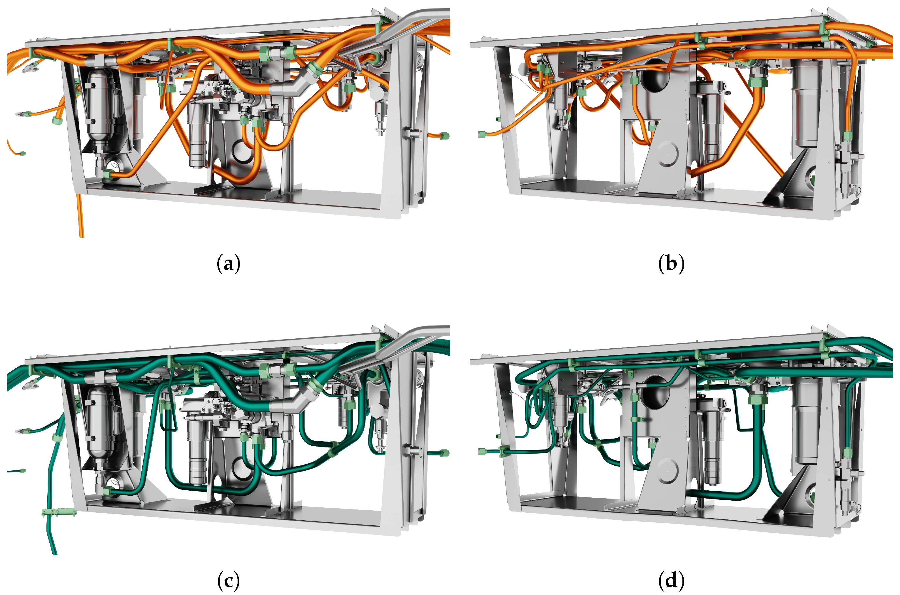
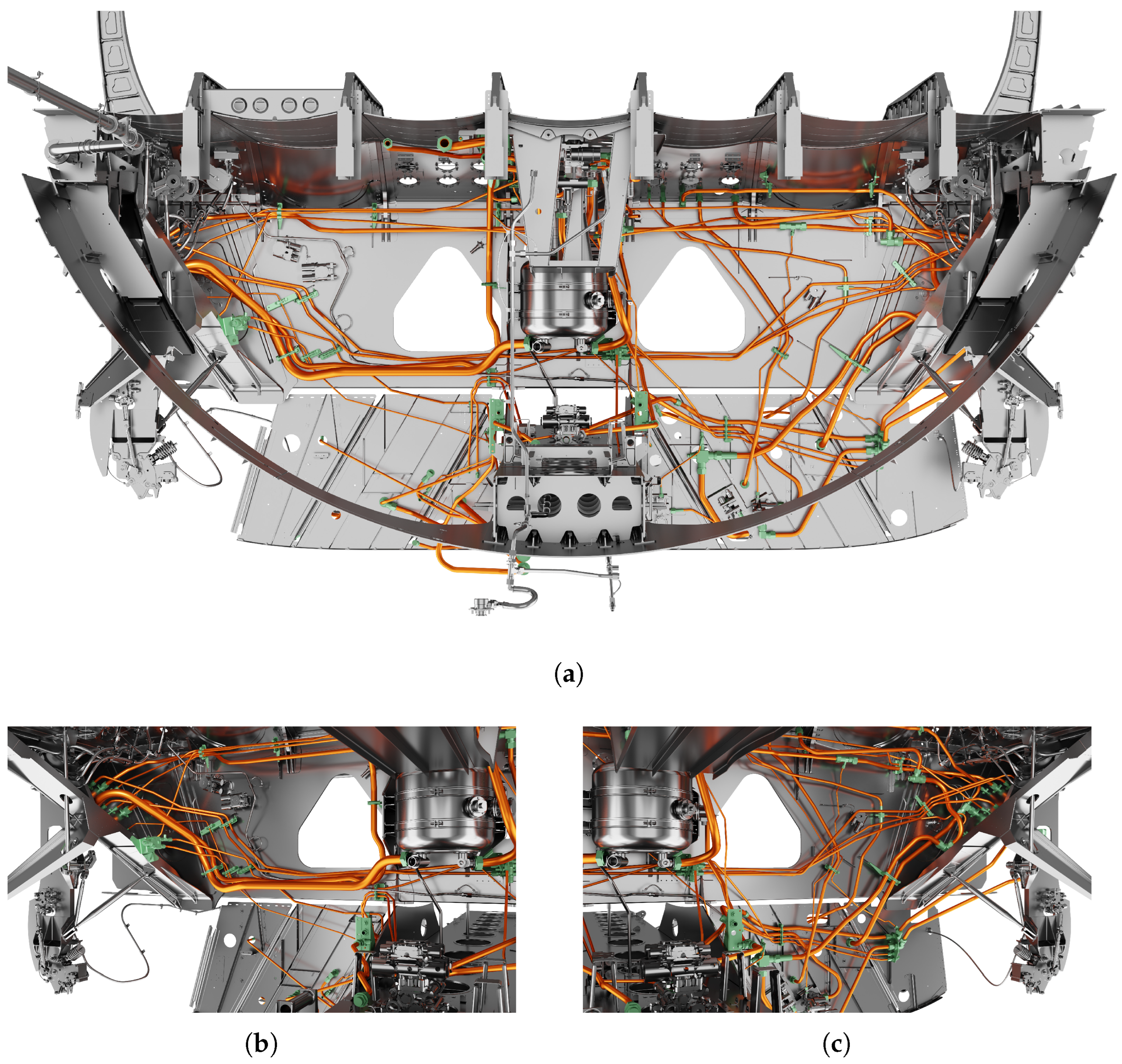
In
Figure 12, an optimization result of 22 pipes with a combined length of approx. 20.7 m and 150 bends is shown in orange color. The automatic pipe generation took 4.5 h on an Intel i5-4440 and 32 GB RAM. The manually designed original solution, shown in green color for comparison, has a length of approx. 22.6 m with 107 bends for the identical pipe connections. Interesting to note is that each automatically generated pipe turns out to be shorter than its manually designed counterpart.
6. Runtime Behaviour
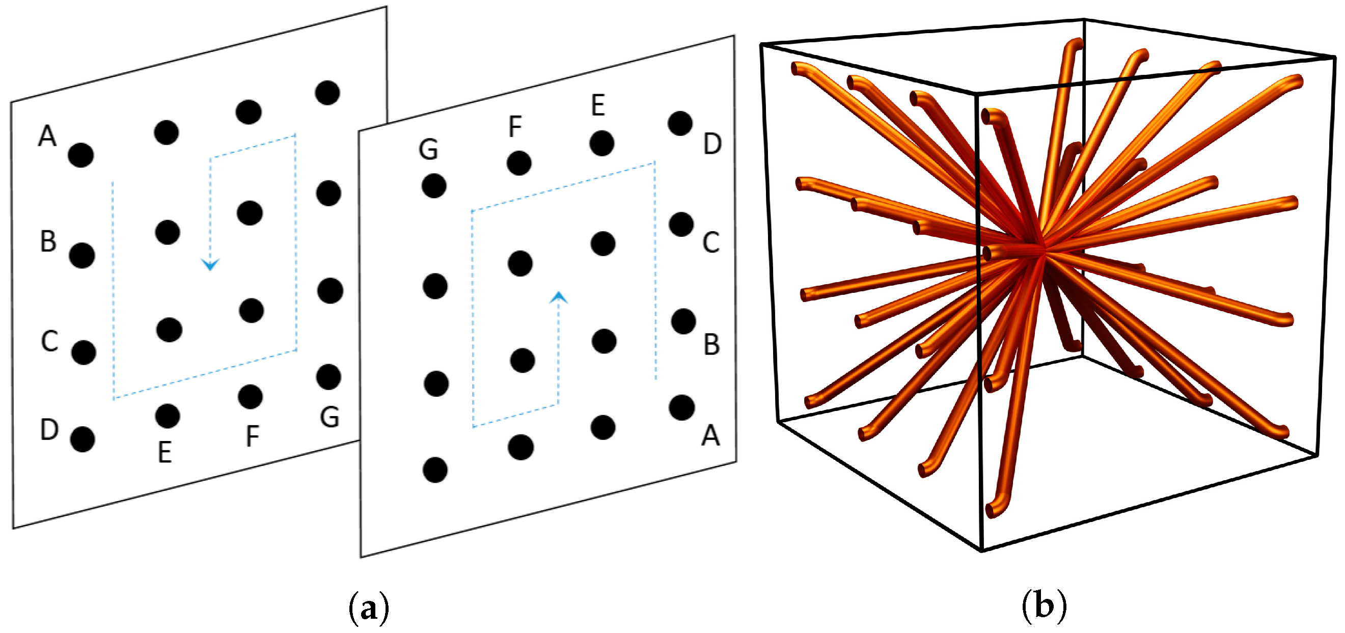
A multitude of settings in a so-called pipe grid were used in the following to empirically investigate the runtime characteristics of the piping algorithm. According to the schematic setting shown in
Figure 13, the corresponding beginnings and endings (i.e., the desired connections
,
,
…) of the pipes are placed in point-symmetric positions on two quadratic grids with a grid size of 1500 mm.
Due to these boundary conditions, all the direct connections between the beginning and the ending of every pipe would theoretically intersect each other in one single point if they were drawn as mathematically straight lines. In consequence, an intended maximum of collisions will occur, thus offering an easily scalable experimental setting to study the runtime behavior of the piping algorithm.
In the following algorithmic investigations the pipes have a diameter of 60 mm, a bending radius of 90 mm and must have a distance between each other of 1 mm. For the investigation the grid size of the quadratic grid was set constant. Additionally an ambient cuboid with an edge length of 1700 mm was used as obstacle. The algorithm was run on a desktop computer with an AMD Ryzen 7 3700x processor and 64 GB RAM. These investigations of the algorithm runtimes is not only used for a scaling investigation as a function of problem size but will also be of interest in future developments of the algorithms based on additional user heuristics to improve the collision handling.
6.1. Runtime Behaviour without Obstacle Interaction
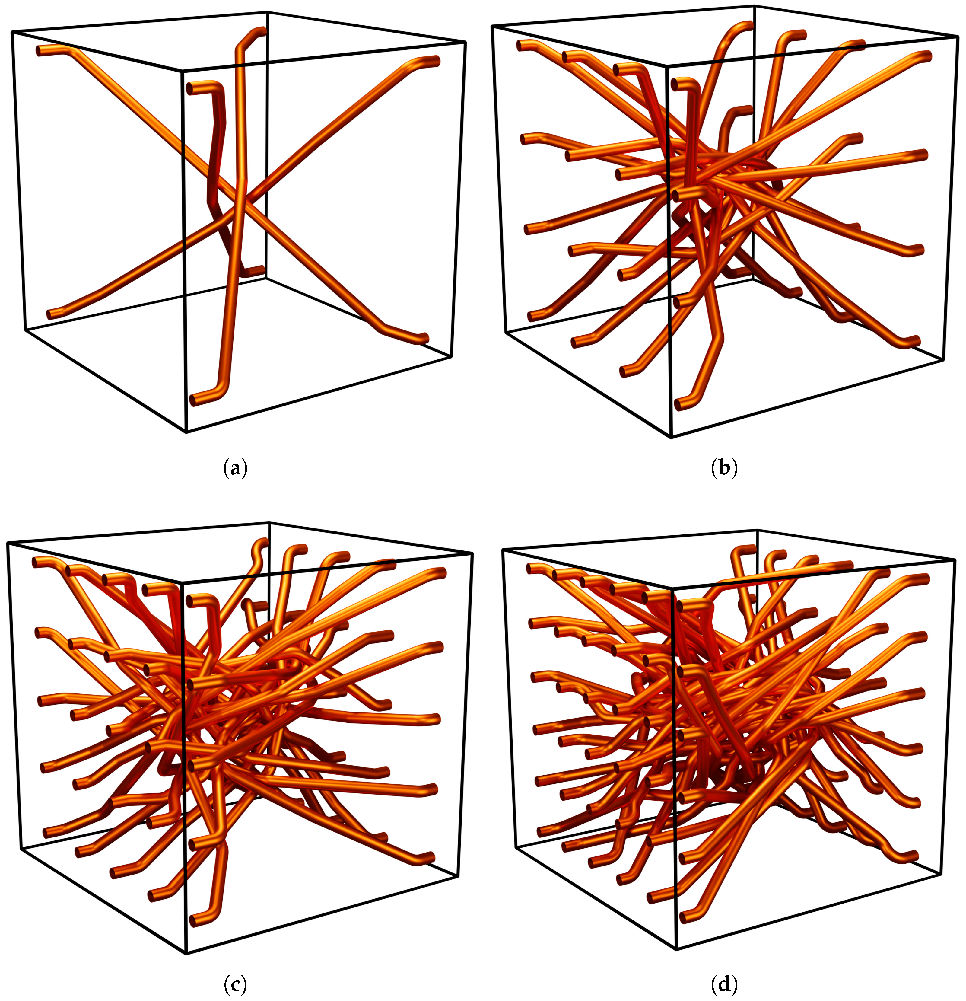
In
Figure 14, the results for different number of pipes are shown. Of the ambient cuboid only the edges are shown in the figure. All the pipes of the piping algorithmic piping solution shown in
Figure 14 are collision free.
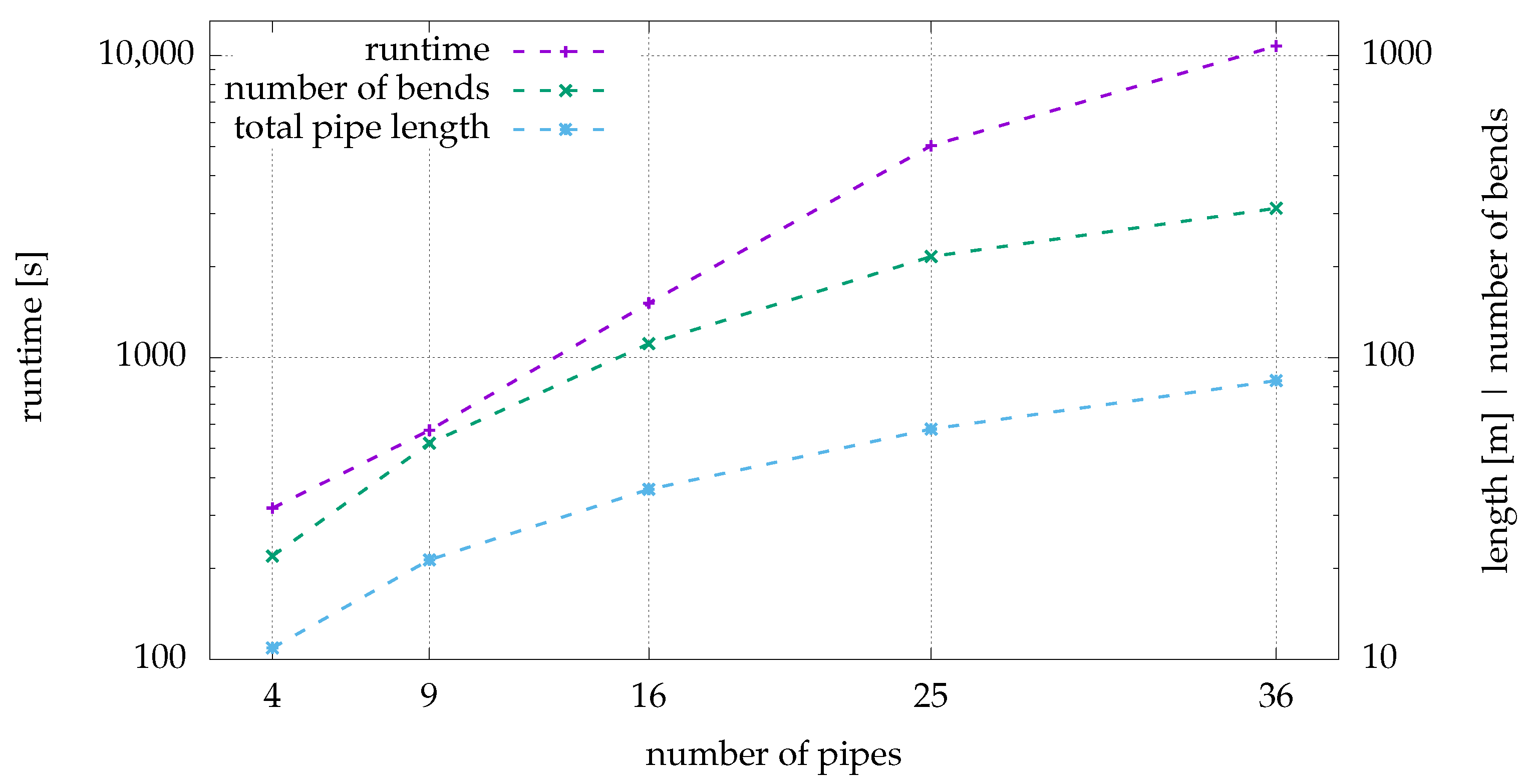
The measured runtime behaviour of the piping algorithm is shown in
Figure 15. The y axes in
Figure 15 are graded in logarithmic, as a result of this an exponential runtime behaviour would lead to a straight line. As it can be clearly seen in the diagram the graph of the runtime has a gradient lower than a straight line would have, therefore it can be said that the runtime is below exponential.
6.2. Runtime Behaviour with Obstacle Interaction
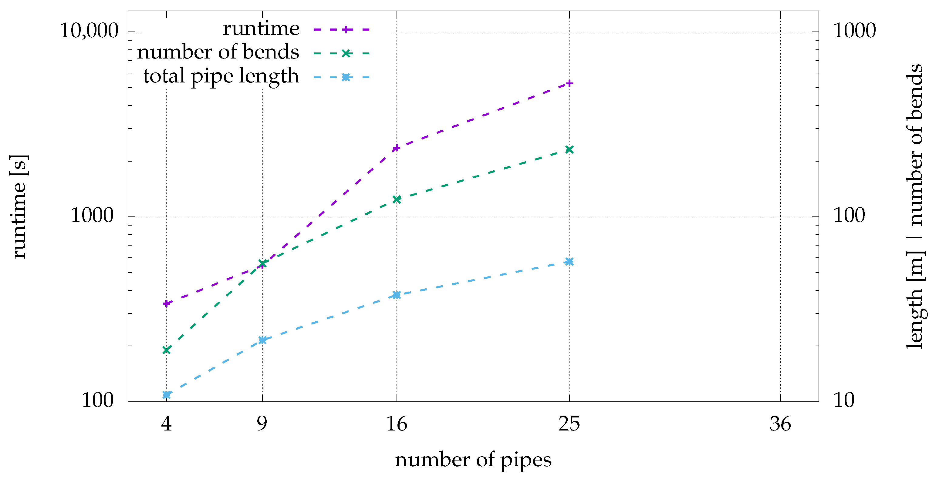
Additionally to the ambient cuboid, a wall with hole was added. The hole has a dimension of 1000 mm × 700 mm and the wall has a thickness of 50 mm. As a result of this only approximately 24% of the crossection area is available for the pipes. The measured runtime behaviour of the piping algorithm as a function of the number of pipes routed is shown in
Figure 16. Due to the shrinkage of the installation space by the obstacle, the algorithm was not able to create valid pipes for a 6 × 6 grid using the same settings like for the other pipe generation. A solution is found only through so-called “virtual fixings”to organize the pipes and thus using the remaining area more efficiently. This is explained in
Section 9. For these and the previous measurements in
Section 6.1 it should be taken into account that the results have been found by simple computation of the difference between the pre and post program execution time stamps.
Similar to the diagram
Figure 15 the y axes in
Figure 16 are graded in logarithmic scale. As it can be seen in the diagram the graph of the runtime has a gradient lower than a straight line would have, therefore it can be said that the runtime is below exponential.
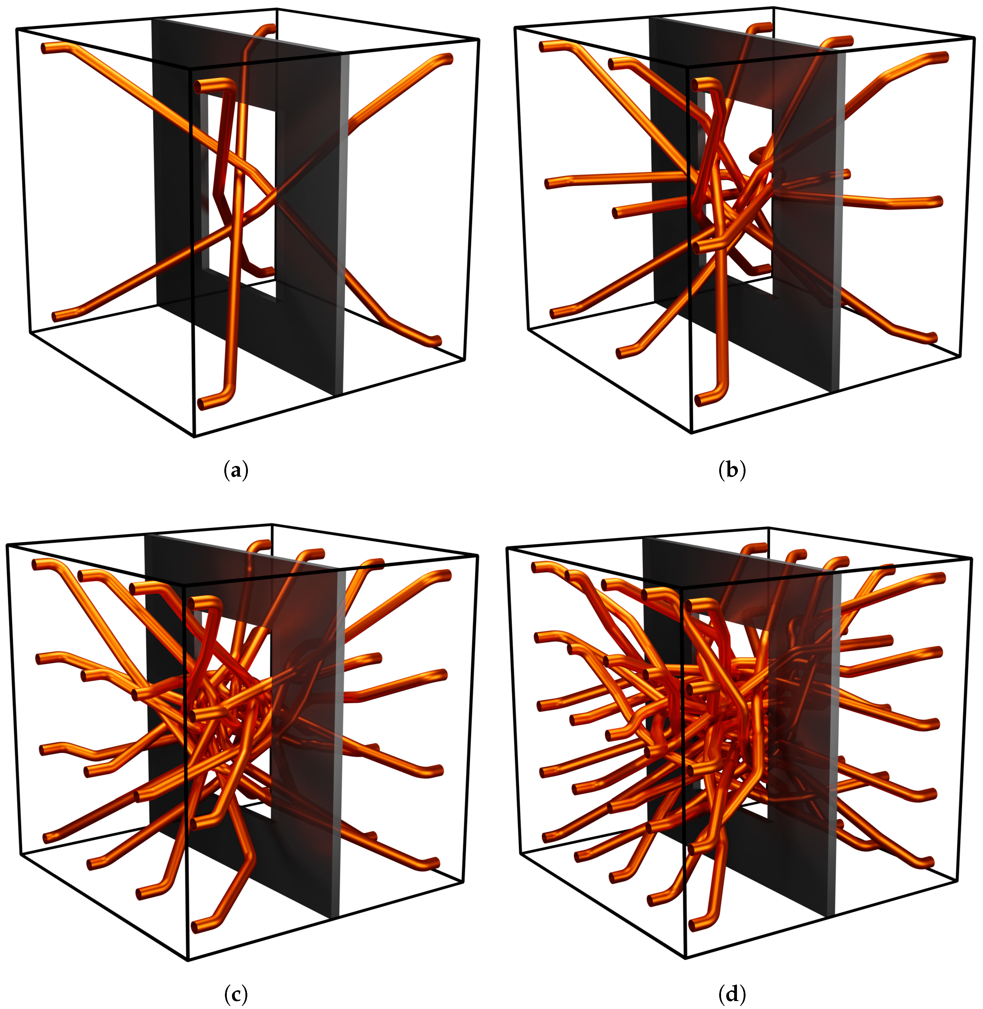
In
Figure 17 the results for different number of pipes are shown. All the pipes of the algorithmic piping solution shown in
Figure 17 are collision free.
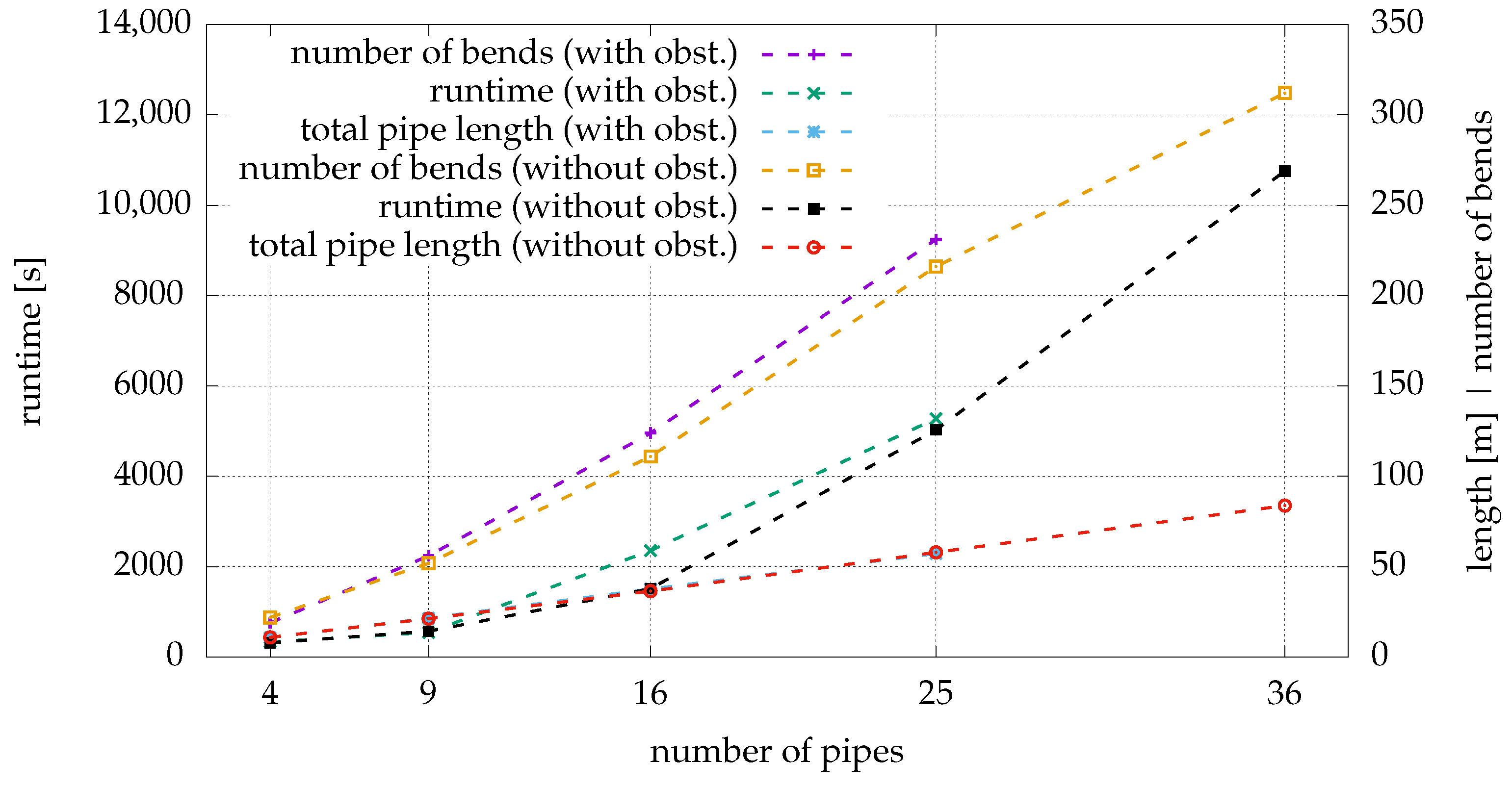
6.3. Comparison of the Piping Results with and without Obstacles
For the investigation of the behaviour of the piping algorithm regarding the influence of an obstacle the pipe routing with the same weightings of the objective criteria, the same number of simulation steps and the same resolution for the simplified obstacle geometry on the same computer was carried out. The results were already shown in the
Section 6.1 and
Section 6.2. In
Figure 18, the runtimes, the number of bends and the total pipe length are compared to each other. It can be seen that the runtimes for the executions with obstacle are higher and also the number of bends increases. This can be explained by the fact that a denser saturation of the available installation space leads to more interactions between the pipes and is therefore more challenging to find a good solution as well as more computational expensive as more distance calculations between the pipes need to be done. A reliable statement about the influence on the total pipe length can not be given in this context as the differences are not judged to be significant.
7. Automated Piping in the Airbus A320 Main Landing Gear Bay
The capabilities of the proposed automation approach are shown by generating pipes in an Airbus A320 main landing gear bay. The involute of the main landing gear and other forbidden stay out zones for the clearance of the maintenance holes have been omitted. A total number of 80 pipes with a combined length of approximately 98 m and 614 bends are shown in
Figure 19.
The generation of these pipes took about one day on an AMD Ryzen 7 3700x processor and 64GB RAM. The solution shown is meant to be a first version of the final pipe work, which can be used as a starting point for the user to make educated decisions to reach the final solution (e.g., adding fixings).
The industrial use cases in
Figure 12 and
Figure 19 illustrate the achievement potential of the presented algorithmic piping automation approach. It could be demonstrated that dozens of pipes which interact with each other and are designed to be manufactured by a bending machine, can be generated automatically in an industrial installation space. Due to the observed runtimes below one day, the presented automated workflow can be integrated in an overall manual industrial design process. It can also be the starting point for future extensions to come closer to the future goal of an holistic model-based aircraft design process relying on a graph-based design languages methodology.
8. Conclusions
A method for an automatic pipe routing which automatically generates pipe designs with an integrated design optimization encoded in graph-based design languages and executable in a design compiler has been presented. The generated pipes can be directly manufactured in a rotary draw bending process.
This manufacturing process requires a pipe consisting of straights and bends in alternating order with specific angles and minimal lengths. Only the start and end positions with the respective direction, the pipe diameter and the properties of the intended bending machine need to be set. In addition, minimal distances of the pipes to obstacles and to each other can be predetermined.
An existing wire harness routing plugin of the Design Compiler 43
® [
1] was used to find a route through the installation space as a first approximation. Based on this route, ray tests are performed to obtain a simplified obstacle geometry. Given this, pipes with different number of bends are estimated. These pipes are optimized with a simulated annealing algorithm, including a just in time assessment of the constraints. The best ones are selected to be shown to the user. For the optimization an evaluation function is proposed, which takes into account multiple different criteria like the length of the pipe and the number of bends. If it occurs that several pipes are too close to each other, these pipes may be grouped and optimized together.
The evaluation criteria are weighted by the user, keeping the user in charge of the overall design decisions. Subsequently to the design optimization, the generated pipes can be automatically reviewed based on the manufacturing requirements and constraints. A runtime investigation with and without obstacles in the sightline of the start and end connection points was carried out. This investigation indicated a below exponential runtime behaviour of the algorithm. The capabilities of this approach are demonstrated and compared to the series pipe work in an Airbus A320 main landing gear bay.
9. Prospects
The automated piping algorithm shown forms a machine-executable, repeatable and reliable basis for a future overall optimization of a highly complex installation space as shown in
Figure 19 compared to the manually created A320 series solution shown in
Figure 20. In this condition of the algorithm different criteria, as described in
Section 4.1, can be taken into account. Future implementations could also include an additional optimization focusing on assembly, integration and tests. The automation approach has the potential to reduce the pipe design effort by one to several orders of magnitude.
Furthermore, the automated piping allows to permanently shift the focus from a detailed, microscopic view on an optimal individual pipe routing back and forth towards a more system level, macroscopic view on the main routes in system installation. Furthermore, any former manually very tedious investigation of alternative equipment changes can now be automatically executed and systematically analysed in a very reasonable amount of time as the runtime for one variant like the one shown in this paper is below one day.
The obstacle geometries shown in
Figure 20 are not yet semantically annotated. In this context, semantic annotation can be understood as a means to address each geometric entity (e.g., a point, a line, a triangle, etc.) with an label. This stems from the fact that the obstacle geometry is part of a manually created aircraft design of years ago. If however the aircraft structure had been designed in a design language, the whole design sequence of the aircraft geometry would be “known” to the piping algorithm which could take this information into account. In the test case described in
Section 6.2 the hole could be an indication to the piping algorithm to align the pipes in the extrusion direction of the hole. This could be done in a regular pattern by virtual fixings.
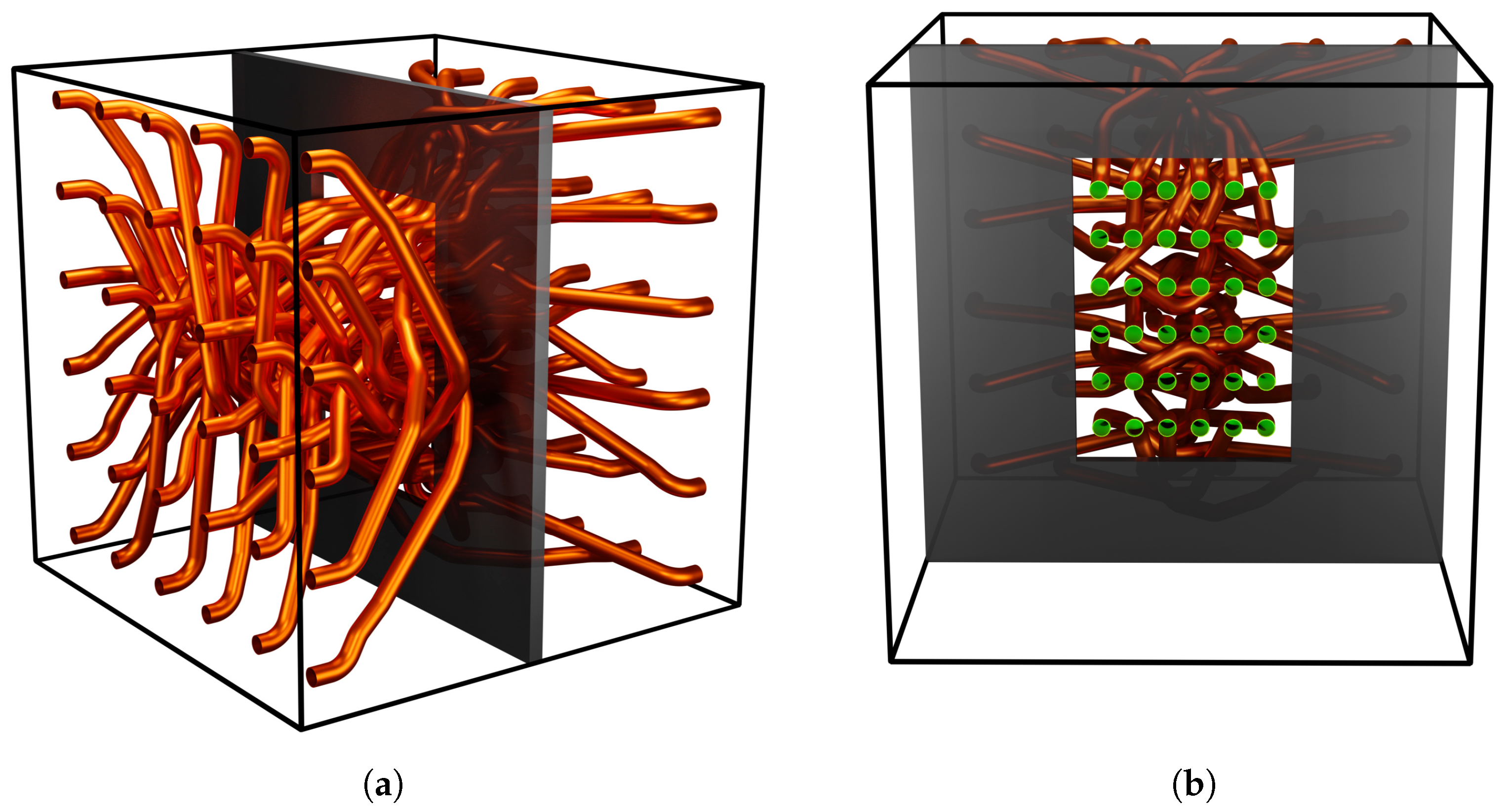
Figure 21a shows an obstacle geometry (i.e., a plate with a hole) created by a rule in a design language and is thus explicitly part of the semantic model. To help “organizing”the pipes crossing the hole, the
Figure 21b shows the result of a fixing rule by means of a manually predefined set of virtual fixings (i.e., the 36 green circles). Using an annotated geometry, this fixing definition could have been also generated automatically. Such additional information may (in comparison to
Figure 17d) “help” the cross section of the hole to be used more efficiently since the pipes are now better aligned. As a result, more pipes can be routed through the same hole or the hole can be made smaller.
This semantic annotation of geometry will open in the future new ways of reasoning on geometry, since the geometry is not only accessible as geometrical entities in the form of points, lines, triangles and every other construct built upon from that. The geometric collision detection check is an important example for such a basic reasoning level on geometry and allows to deduce already important information (i.e., the information that the geometrical setting is either collision-free or exhibits a collision of x mm) from that. The aforementioned semantic annotation will allow to reason on geometry on a higher reasoning level, e.g., knowing that “pipes can only pass through holes and never through walls or any other part of a solid structure” will allow to automate even more complex planning tasks of pipes routes using higher levels of abstraction. Such developments will be part of future planned improvements of the automated piping algorithm.
Author Contributions
Conceptualization, M.N., S.K., B.K. and S.R.; Data curation, S.K.; Methodology, M.N. and S.R.; Project administration, B.K. and S.R.; Software, M.N.; Supervision, B.K. and S.R.; Visualization, M.N.; Writing—original draft, M.N., S.K. and S.R.; Writing—review & editing, M.N., S.K., B.K. and S.R. All authors have read and agreed to the published version of the manuscript.
Funding
The work shown here as a part of the H2020 CS2-Project PHAROS has received funding from the Clean Sky 2 Joint Undertaking (JU) under grant agreement number 865044 (see
https://cordis.europa.eu/project/id/865044 (accessed on 13 January 2022) for details). The JU receives support from the European Union’s Horizon 2020 research and innovation programme and the Clean Sky 2 JU members other than the Union. The content of this paper reflects only the author’s view and the JU is not responsible for any use that may be made of the information it contains.
Acknowledgments
The authors would like to thank the Airbus Operations GmbH, Hamburg, for providing the
Figure 2 and
Figure 20.
Conflicts of Interest
The authors declare no conflict of interest. The funders had no role in the design of the study; in the collection, analyses, or interpretation of data; in the writing of the manuscript, or in the decision to publish the results.
References
- IILS mbH 2021 Design Compiler 43®. Ingenieurgesellschaft für intelligente Lösungen und Systeme mbH. Available online: https://www.iils.de (accessed on 14 January 2022).
- Groß, J.; Rudolph, S. Modeling graph-based satellite design languages. Aerosp. Sci. Technol. 2016, 49, 63–72. [Google Scholar] [CrossRef]
- Riestenpatt, G.; Richter, M.; Rudolph, S. A scientific discourse on creativity and innovation in the formal context of graph-based design languages. In Proceedings of the 13th Anniversary Heron Island Conference Workshop on Computational and Cognitive Models of Creative Design (HI‘19), Heron Island, QLD, Australia, 15–18 December 2019. [Google Scholar]
- Tonhäuser, C.; Rudolph, S. Individual Coffee Maker Design Using Graph-Based Design Languages. In Proceedings of the 7th Conference on Design Cognition and Computing (DCC 2016), Evanston, IL, USA, 27–29 June 2016. [Google Scholar]
- Walter, B.; Kaiser, D.; Rudolph, S. From Manual to Machine-executable Model-based Systems Engineering via Graph-based Design Languages. In Proceedings of the 7th International Conference on Model-Driven Engineering and Software Development (MODELSWARD 2019), Prague, Czech Republic, 20–22 February 2019; pp. 203–210. [Google Scholar]
- Voss, C.; Petzold, F.; Rudolph, S. Graph Transformation in Engineering Design: An Overview of the Last Decade. AIEDAM 2022. submitted. [Google Scholar]
- Chakrabarti, A.; Shea, K.; Stone, R.; Cagan, J.; Campbell, M.; Hernandez, N.; Wood, K. Computer-based design synthesis research: An overview. J. Comput. Inf. Sci. Eng. 2011, 11, 21003. [Google Scholar] [CrossRef]
- Ozkaya, M.; Akdur, D. What do practitioners expect from the meta-modeling tools? A survey. J. Comput. Lang. 2021, 63, 101030. [Google Scholar] [CrossRef]
- Sebastián, G.; Gallud, J.A.; Tesoriero, R. Code generation using model driven architecture: A systematic mapping study. J. Comput. Lang. 2020, 56, 100935. [Google Scholar] [CrossRef]
- Nieke, M.; Hoff, A.; Seidl, C.; Schaefer, I. Augmenting metamodels with seamless support for planning, tracking, and slicing model evolution timelines. J. Comput. Lang. 2021, 63, 101031. [Google Scholar] [CrossRef]
- Cagan, J.; Shimada, K.; Yin, S. A survey of computational approaches to three-dimensional layout problems. Comput.-Aided Des. 2002, 34, 597–611. [Google Scholar] [CrossRef] [Green Version]
- De Bont, F.; Aarts, E.; Meehan, P.; O’Brian, C. Placement of shapeable blocks. Philips J. Res. 1988, 43, 1–22. [Google Scholar]
- Goldreich, O. P, NP and NP-Completeness: The Basics of Computational Complexity; Cambridge University Press: Cambridge, UK, 2010. [Google Scholar]
- Kirkpatrick, S.; Gelatt, C.; Vecchi, M. Optimization by Simulated Annealing. Science 1983, 220, 671–680. [Google Scholar] [CrossRef] [PubMed]
- Rudolph, S. Know-How Reuse in the Conceptual Design Phase of Complex Engineering Products—Or: ‘Are you still constructing manually or do you already generate automatically’? In Proceedings of the Conference on Integrated Design and Manufacture in Mechanical Engineering 2006 (IDMME 2006), Grenoble, France, 17–19 May 2006. [Google Scholar]
- Dinkelacker, J.; Kaiser, D.; Panzeri, M.; Parmentier, P.; Neumaier, M.; Tonhäuser, C.; Rudolph, S. System Integration based on packaging, piping and harness routing automation using graph-based design languages. In Proceedings of the Deutscher Luft-und Raumfahrtkongress 2021, Bremen, Germany, 31 August–2 September 2021. [Google Scholar]
- Rudolph, S. A Semantic Validation Scheme for Graph-Based Engineering Design Grammars. In Proceedings of the Design Computing and Cognition (DCC‘06), Dordrecht, The Netherlands, 10–12 July 2006; Gero, J., Ed.; Springer: Berlin/Heidelberg, Germany, 2006; pp. 541–560. [Google Scholar]
- VDI 3430:2014-06; Rotary Draw Bending of Profiles. Beuth Verlag: Berlin, Germany, 2014.
- Kang, S.; Myung, S.; Han, S. A Design expert system for auto-routing of ship pipes. J. Ship Prod. 1999, 15, 1–9. [Google Scholar] [CrossRef]
- Niu, W.; Sui, H.; Niu, Y.; Cai, K.; Gao, W. Ship Pipe Routing Design Using NSGA-II and Coevolutionary Algorithm. Math. Probl. Eng. 2016, 2016, 7912863. [Google Scholar] [CrossRef] [Green Version]
- Qu, Y.; Jiang, D.; Zhang, X. A New Pipe Routing Approach for Aero-Engines by Octree Modeling and Modified Max-Min Ant System Optimization Algorithm. J. Mech. 2018, 34, 11–19. [Google Scholar] [CrossRef]
- Kim, S.; Choi, T.; Kim, S.; Kwon, T.; Lee, T. Sequential graph-based routing algorithm for electrical harnesses, tubes, and hoses in a commercial vehicle. J. Intell. Manuf. 2021, 32, 912–933. [Google Scholar] [CrossRef]
- Thantulage, G. Ant Colony Optimization Based Simulation of 3D Automatic Hose/Pipe Routing. Ph.D. Thesis, School of Engineering and Design Brunel University, Uxbridge, UK, 2009. [Google Scholar]
- Liu, Q.; Jiao, G. A Pipe Routing Method Considering Vibration for Aero-Engine Using Kriging Model and NSGA-II. IEEE Access 2018, 6, 6286–6292. [Google Scholar] [CrossRef]
- Wang, H.; Zhao, C.; Yan, W.; Feng, X. Three-Dimensional Multi-Pipe Route Optimization Based on Genetic Algorithms. In International Federation for Information Processing (IFIP), Knowledge Enterprise: Intelligent Strategies in Product Design, Manufacturing, and Management; Wang, K., Kovacs, G., Wozny, M., Fang, M., Eds.; Springer: Boston, MA, USA, 2006; Volume 207, pp. 177–183. [Google Scholar]
- Lee, K. Optimal System Design with Geometric Considerations. Ph.D. Thesis, University of Michigan, Ann Arbor, MI, USA, 2014. [Google Scholar]
- Szykman, S.; Cagan, J. Synthesis of Optimal Nonorthogonal Routes. ASME. J. Mech. Des. 1996, 118, 419–424. [Google Scholar] [CrossRef]
- Liu, Q.; Tang, Z.; Liu, H.; Yu, J.; Ma, H.; Yang, Y. Integrated Optimization of Pipe Routing and Clamp Layout for Aeroengine Using Improved MOALO. Int. J. Aerosp. Eng. 2021, 2021, 6681322. [Google Scholar] [CrossRef]
- Yuan, H.; Yu, J.; Jia, D.; Liu, Q.; Ma, H. Group-based multiple pipe routing method for aero-engine focusing on parallel layout. Front. Mech. Eng. 2021, 1–16. [Google Scholar] [CrossRef]
- Eheim, M.; Kaiser, D.; Weil, R. On Automation Along the Automotive Wire Harness Value Chain. In Advances in Automotive Production Technology—Theory and Application, Proceedings of the Stuttgart Conference on Automotive Production (SCAP2020), Stuttgart, Germany, 9–10 November 2020; Weißgraeber, P., Heieck, F., Ackermann, C., Eds.; Springer: Berlin/Heidelberg, Germany, 2021; pp. 178–186. [Google Scholar]
- Garcia-Castellanos, D.; Lombardo, U. Poles of Inaccessibility: A Calculation Algorithm for the Remotest Places on Earth. Scott. Geogr. J. 2007, 123, 227–233. [Google Scholar] [CrossRef]
- Farhat, C.; Lesoinne, M. Two efficient staggered algorithms for the serial and parallel solution of three-dimensional nonlinear transient aeroelastic problems. Comput. Methods Appl. Mech. Eng. 2000, 182, 499–515. [Google Scholar] [CrossRef]
- Weyland, D. Simulated Annealing, its Parameter Settings and the Longest Common Subsequence Problem. In Proceedings of the 10th Annual Conference on Genetic and Evolutionary Computation 2008, Atlanta, GA, USA, 12–16 July 2008; pp. 803–810. [Google Scholar]
- Rudolph, S. 2019 Physical Architecture Optimization System (PHAROS). H2020 CS2 Grant Proposal, Part B.I (Confidential, Unpublished). Available online: https://cordis.europa.eu/project/id/865044 (accessed on 14 January 2022).
Figure 1.
MBSE V-Model (left) including validation and verification pattern (right).
Figure 1.
MBSE V-Model (left) including validation and verification pattern (right).
Figure 2.
Airbus A320 series solution mounting rack (© 2022 AIRBUS Operations GmbH).
Figure 2.
Airbus A320 series solution mounting rack (© 2022 AIRBUS Operations GmbH).
Figure 3.
Rotary draw bending process.
Figure 3.
Rotary draw bending process.
Figure 4.
Exemplary installation space: Airbus A320 mounting rack. (a) Empty installation space, (b) Paths through the installation space, (c) Automatically generated pipes, (d) Manually designed pipes.
Figure 4.
Exemplary installation space: Airbus A320 mounting rack. (a) Empty installation space, (b) Paths through the installation space, (c) Automatically generated pipes, (d) Manually designed pipes.
Figure 6.
Airbus A320 mounting rack geometry with margin in all spatial directions.
Figure 6.
Airbus A320 mounting rack geometry with margin in all spatial directions.
Figure 7.
Boundary exploration in one crossection.
Figure 7.
Boundary exploration in one crossection.
Figure 8.
Exemplary rounded polyline.
Figure 8.
Exemplary rounded polyline.
Figure 9.
Class diagram (snippet).
Figure 9.
Class diagram (snippet).
Figure 10.
Exemplary graph of a PipePath consisting of Straights and Bends.
Figure 10.
Exemplary graph of a PipePath consisting of Straights and Bends.
Figure 11.
Modification strategies.
Figure 11.
Modification strategies.
Figure 12.
Automatically generated (orange) and manually designed pipes (green) in an Airbus A320 mounting rack. (a) Automatically generated pipes (seen from the left side), (b) Automatically generated pipes (seen from the right side), (c) Manually designed pipes (seen from the left side), (d) Manually designed pipes (seen from the right side).
Figure 13.
Connection schema on opposite grids with point-symmetric positions. (a) Connection schema with point-symmetric positions to enforce collisions. (b) 4 × 4 pipes with enforced collisions.
Figure 13.
Connection schema on opposite grids with point-symmetric positions. (a) Connection schema with point-symmetric positions to enforce collisions. (b) 4 × 4 pipes with enforced collisions.
Figure 14.
Algorithmic pipe solutions in a box. (a) 2 × 2 pipes, (b) 4 × 4 pipes, (c) 5 × 5 pipes, (d) 6 × 6 pipes.
Figure 14.
Algorithmic pipe solutions in a box. (a) 2 × 2 pipes, (b) 4 × 4 pipes, (c) 5 × 5 pipes, (d) 6 × 6 pipes.
Figure 15.
Relationship between the number of pipes, the runtime, the number of bends and the total pipe length.
Figure 15.
Relationship between the number of pipes, the runtime, the number of bends and the total pipe length.
Figure 16.
Relationship between the number of pipes, the runtime, the number of bends and the total pipe length with obstacle.
Figure 16.
Relationship between the number of pipes, the runtime, the number of bends and the total pipe length with obstacle.
Figure 17.
Algorithmic pipe solutions in a box with additional obstacle. (a) 2 × 2 pipes, (b) 3 × 3 pipes, (c) 4 × 4 pipes, (d) 5 × 5 pipes.
Figure 17.
Algorithmic pipe solutions in a box with additional obstacle. (a) 2 × 2 pipes, (b) 3 × 3 pipes, (c) 4 × 4 pipes, (d) 5 × 5 pipes.
Figure 18.
Comparison of the piping results without and with obstacle.
Figure 18.
Comparison of the piping results without and with obstacle.
Figure 19.
Automated pipe routing in an Airbus A320 landing gear bay. (a) Overview in flight direction, (b) Detail left side, (c) Detail right side.
Figure 19.
Automated pipe routing in an Airbus A320 landing gear bay. (a) Overview in flight direction, (b) Detail left side, (c) Detail right side.
Figure 20.
Piping series solution in an Airbus A320 main landing gear bay (© 2022 Airbus). (a) left side main landing gear bay, (b) right side main landing gear bay.
Figure 20.
Piping series solution in an Airbus A320 main landing gear bay (© 2022 Airbus). (a) left side main landing gear bay, (b) right side main landing gear bay.
Figure 21.
Test case with manual defined virtual fixings. (a) 6 × 6 pipes, (b) half of 6 × 6 pipes hidden.
Figure 21.
Test case with manual defined virtual fixings. (a) 6 × 6 pipes, (b) half of 6 × 6 pipes hidden.
Table 1.
Exemplary automatically generated bend table.
Table 1.
Exemplary automatically generated bend table.
| ID | x | y | z | Distance | Straight Length | Bend Angle | Bend Radius |
|---|
| S.0 | 0.0 | 0.0 | 0.0 | - | - | - | - |
| B.1 | 99.746 | 0.0 | 0.0 | 99.746 | 58.633 | | 90.0 |
| B.2 | 292.924 | 146.471 | 168.194 | 295.06 | 238.27 | | 90.0 |
| B.3 | 653.16 | 764.793 | 865.078 | 998.869 | 971.048 | | 90.0 |
| B.4 | 1332.909 | 1500.0 | 1500.0 | 1185.628 | 1126.615 | | 90.0 |
| E.5 | 1500.0 | 1500.0 | 1500.0 | 167.091 | 120.223 | - | - |
| Publisher’s Note: MDPI stays neutral with regard to jurisdictional claims in published maps and institutional affiliations. |
© 2022 by the authors. Licensee MDPI, Basel, Switzerland. This article is an open access article distributed under the terms and conditions of the Creative Commons Attribution (CC BY) license (https://creativecommons.org/licenses/by/4.0/).


