Inlet Gap Influence on Low-Frequency Flow Unsteadiness in a Centrifugal Fan

Abstract

In this study, unsteady low-frequency characteristics in a voluteless low-speed centrifugal fan operating at a high mass flow rate are studied with improved delayed detached eddy simulation (IDDES). This study is motivated by a recent finding that the non-uniformly distributed pressure inside this type of fan could be alleviated by improving the gap geometry. The present simulation results show that the velocity magnitudes of the gap have distinct low and high regions. Intensive turbulent structures are developed in the low-velocity regions and are swept downstream along the intersection between the blade and shroud, on the pressure side of the blade. Eventually, the turbulence gives rise to a high-pressure region near the blade’s trailing edge. This unsteady flow behavior revolves around the fan rotation axis. Additionally, its period is 5% of the fan rotation speed, based on the analysis of the time history of the gap velocity magnitudes and the evolution of the high-pressure region. The same frequency of high pressure was also found in previous experimental measurements. To the authors’ knowledge, this is the first time that the trigger of the gap turbulence, i.e., the unsteady local low velocity, has been determined.

1. Introduction

Since we spend the majority of our time (up to 90%) inside, [1], indoor environmental quality (IEQ) is important to quality of life. IEQ is usually evaluated in terms of temperature, CO₂ content, and humidity, and especially sound quality [2,3]. Direct negative impacts of noise include loss of hearing and tinnitus, and indirect effects include stress, sleep disturbance, annoyance, etc. [4]. For example, according to [5], children´s cognitive development is impaired by long-term noise exposure.

The IEQ is dependent on equipment that controls indoor air and sound quality, namely a heating, ventilation, and air-conditioning (HVAC) system. In modern HVAC systems, low-speed voluteless centrifugal fans are often used, and these types of fans are known as dominant noise generators, especially when producing tonal noise. As this type of fan does not have a volute (i.e., a casing), we refer to this design as ‘voluteless’ in this study. Based on the pioneering study of Ffowcs Williams and Hawkings [6], the blades of the fan are subjected to fluctuating flow quantities such as density and pressure, which are major sources of tonal noise.

Modern HVAC systems operate as variable air volume (VAV) systems, which means that the HVAC system operates from the lowest (almost 0) to the highest offered mass flow rate. In this study, the mass flow rate of the fan ranges from 0 to 0.55 kg/s. The maximum efficiency mass flow rate is named $Q_E$, and mass flow rates larger than $Q_E$, are called high mass flow rates.

The fan as a whole is rotating, while the flow is guided into it with a duct that is stationary. Between the rotating and stationary parts, there is a clearance, referred to as the inlet gap in this study. Due to the difference of the pressure inside and outside the fan, air passing through the gap becomes a jet flow locally, which accounts for flow separation near the shroud according to Lee [7]. Later studies further demonstrated this effect [8,9]. By plotting streamlines through the gap, it was found that the jet flow finally leads to recirculation near the joint position between the fan shroud and the blade trailing edge (BTE). The flow recirculation creates significant turbulence, as implied by the distribution of turbulence kinetic energy (TKE) [9]. Additionally, the shroud geometry is not streamlined; flow separation would also be generated due to adverse pressure gradient, as demonstrated in experiments [10,11]. Pavesi et al. [12] observed that a voluteless centrifugal fan has a strong vorticity field in the blade passage near the trailing edge of the blade. The unstable passage flow causes periodic pressure fluctuations on the blade surfaces. Moreover, the shroud wall shear stress introduces additional rotational momentum into the flow near the shroud walls. In other words, the boundary layer flow swirls before it hits the blades. The same finding was also reported in [13]. At the blade-passing frequency (BPF) of voluteless low-speed centrifugal fans, tonal noise is created when turbulence, generated at the gap, interacts with the blade leading edge (BLE) according to previous studies [14,15]. BPF frequencies are usually well above 100 Hz. However, fans can generate low-frequency noise. According to [16] HVAC systems can generate infrasound, which is low-frequency noise (below 20 Hz). It was reported that this leads to vibrations that resonate through building materials, leading to sick building syndrome, which can cause headaches and dizziness. Low-frequency noise generated by centrifugal fans is often due to rotating stalls or surges [17]. Zheng and Liu [18] found that a mild surge of a centrifugal compressor can occur at a medium mass flow rate ($<Q_E$), and the mild surge vanishes and a deep surge starts as the mass flow rate is reduced. As reported by He and Zheng [19], the mild surge is in a sinusoidal wave at the natural harmonic frequency. The rotation speed for the surge has been investigated in several studies. Haynes et al. [20] and Paduano et al. [21], reported that the mild surge has a relatively small amplitude and rotates in the circumferential direction with a speed of 20–50% of the fan speed. In an experimental and numerical study on surge [22], it was shown that even at a higher mass flow rate ($Q=1.3Q_E$), a periodic low-frequency pressure fluctuation was detected. It was found that the pressure fluctuations disappeared as the gap was redesigned [15]. However, the physical mechanisms were not discussed in these studies.

As summary of the literature above, the gap geometry affects the voluteless fan aerodynamics and aeroacoustics. The reason is that the forces on the fan blade are influenced by the turbulent flow evolving from the gap. The surge and stall are predominant low-frequency fluctuations at middle to low mass flow rates. However, to date, it has not been clarified what causes the low-frequency fluctuations at higher mass flow rates ($>Q_E$).

A voluteless fan has been simulated using unsteady Reynolds-averaged Navier–Stokes (URANS) equations [9,23]. Additionally, the aerodynamic forces obtained from the simulations were accurately predicted compared to test data [9]. This numerical method has a disadvantage in that transient turbulent structures cannot be resolved, although large-scale unsteady content is captured [14]. In contrast, most turbulent fluctuations can be resolved with the improved delayed detached eddy simulation (IDDES) which models sub-grid scale fluctuations [24].

In the current study, the main objective is the exploration of physical mechanisms that are associated with the formation of low-frequency fluctuations inside the fan at higher mass flow rates $Q>Q_E$. The flow passing through the fan gap will be studied to understand its effects on the onset of the turbulence. In addition, the evolution of the low-frequency unsteadiness associated with flow separation, which occurs specifically at one blade and revolves around the fan rotation axis, will be clarified. The numerical simulations are carried out using IDDES and the k-ω SST turbulence model.

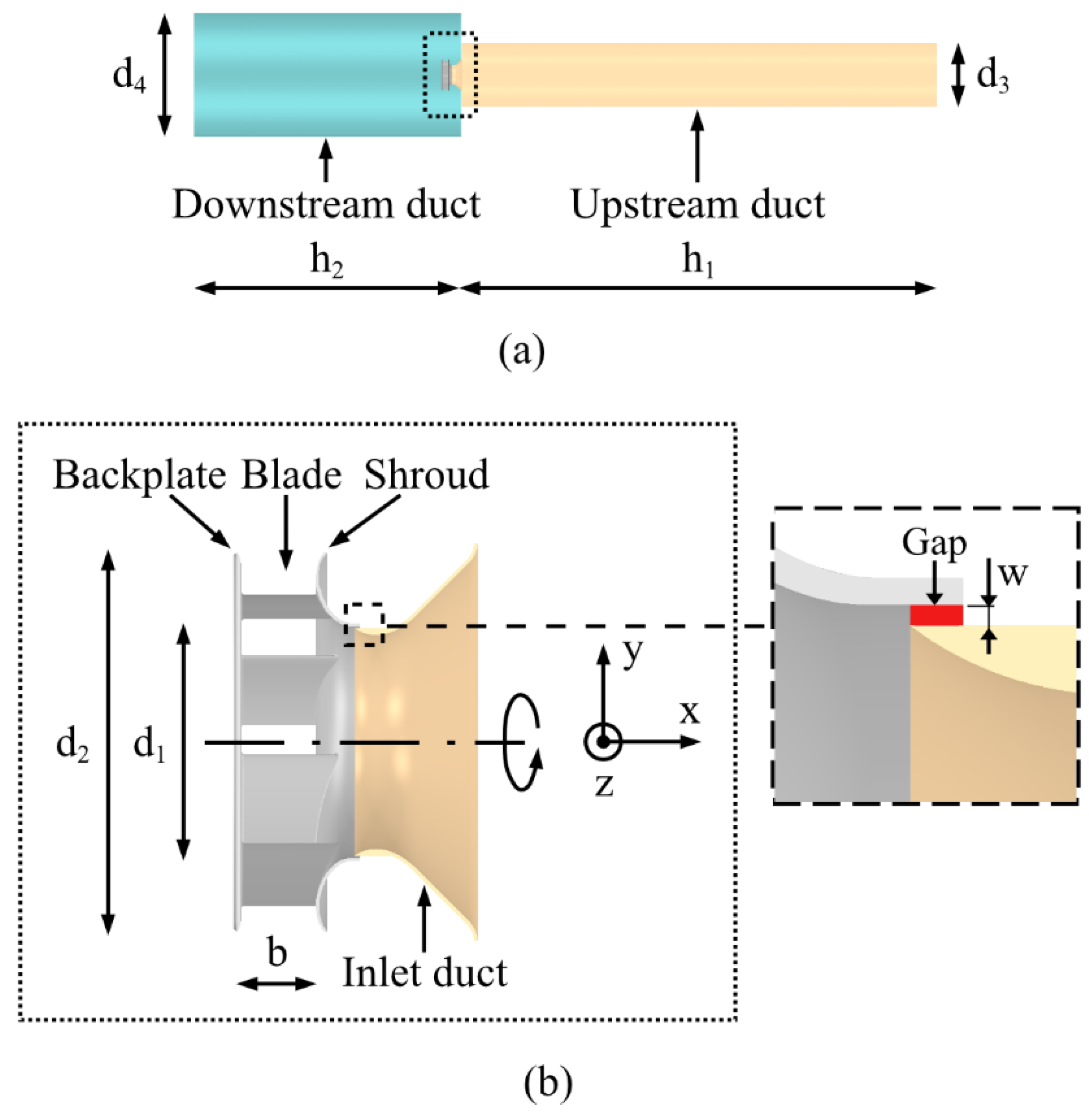
2. Application Cases

The voluteless centrifugal fan and the duct on the fan inlet side are illustrated in Figure 1. The fan is a benchmark that represents most of the characteristics of this type of fan, which has been previously examined in [14,15]. The inlet duct is assembled onto another duct located upstream of it, while the diameter of the inlet duct is smaller than that of the upstream duct. To submerge the inlet duct into the fan intake, the inlet duct outlet has a slightly smaller diameter than the fan intake forming the fan gap. Note that the geometric setup of the ducts is different from real applications, because this setup is specifically designed to reduce the geometry complexity for numerical simulations, but retain major flow and acoustic characteristics.

Table 1. The key parameters of the voluteless fan.

d1	d2	d3	d4	b	h1	h2	w
0.165 m	0.268 m	0.6 m	1.1 m	0.053	4.0 m	2.3 m	1.5 mm

lists the geometry parameters of the fan, which are also marked out in Figure 1.

With the rotation speed of the fan set to 2800 rpm, the maximum efficiency point occurs at $Q_E=0.36 \mathrm{kg}/\mathrm{s}$. The operating point $(Q_{OP})$ in this study is the same as in [14,15], where the mass flow rate was 0.467 kg/s, leading to a pressure rise of 269.65 Pa based on the fan characteristic curve in Figure 2. $Q_{OP}=1.3Q_E$ which is a high mass flow rate.

3. Numerical Method

3.1. Method of Computational Fluid Dynamics

In this study, the CFD simulations are performed using the commercial software STAR-CCM+ [25].

The governing equations of flow are:

$$\frac{\partial \rho }{\partial t}+\nabla ·\left(\rho \mathit{u}\right)=0,$$

$$\frac{\partial \left(\rho \mathit{u}\right)}{\partial t}+\nabla ·\left(\rho \mathit{u}\otimes \mathit{u}\right)=-\nabla p+\nabla ·\mathit{\tau },$$

$$\frac{\partial }{\partial t}\left(\rho E\right)+\nabla ·\left(\rho E\mathit{u}\right)=\nabla ·\left(k\nabla T\right)-\nabla ·\left(\rho ·\mathit{u}\right)+\nabla ·\left(\mathit{u}·\mathit{\tau }\right)$$

(1)

where e is the internal energy, and $E=e+\mathit{u}·\mathit{u}/2$, for the total energy.

For compressible flow, the stress tensor $\mathit{\tau }$ is written to be:

$$\mathit{\tau }=\mu \left[\nabla \mathit{u}+{\left(\nabla \mathit{u}\right)}^T\right]-\frac{2}{3}\mu \left(\nabla ·u\right)I$$

(2)

where $\mu$ is the dynamic viscosity, and $\mu \left[\nabla u+{\left(\nabla u\right)}^T\right]$ is associated with velocity gradients [26].

The air is assumed to be an ideal gas. A segregated finite volume method with the Semi-Implicit Method for Pressure-Linked Equations (SIMPLE) algorithm [27] is used to solve the governing equations. The numerical schemes and discretization refer to the study [16,17], which has also been validated in [9,28].

The IDDES takes the k-ω SST turbulence model [29]. It has been successfully applied to the simulation of rotating machinery; for example, the studies in [30,31]. In the IDDES, the dissipation in the TKE $\left(k\right)$ is corrected with a hybrid length-scale

$${\tilde{l}}_{DDES}={\tilde{f}}_d\left(1+f_e\right)l_{RANS}+\left(1-{\tilde{f}}_d\right)l_{LES}$$

(3)

where $l_{RANS}$ is the length scale of $l_{LES}$ are the Reynolds-averaged Navier–Stokes equations (RANS), and $l_{LES}$ is the length scale of LES. The ${\tilde{f}}_d$ function blends between RANS and LES and the ${\tilde{f}}_e$ slightly enhances the RANS content in the RANS region. The equations of the IDDES turbulence model, as well as the coefficients, can be found in [14,15]. To avoid repetition, they are reproduced here.

3.2. Numerical Setup

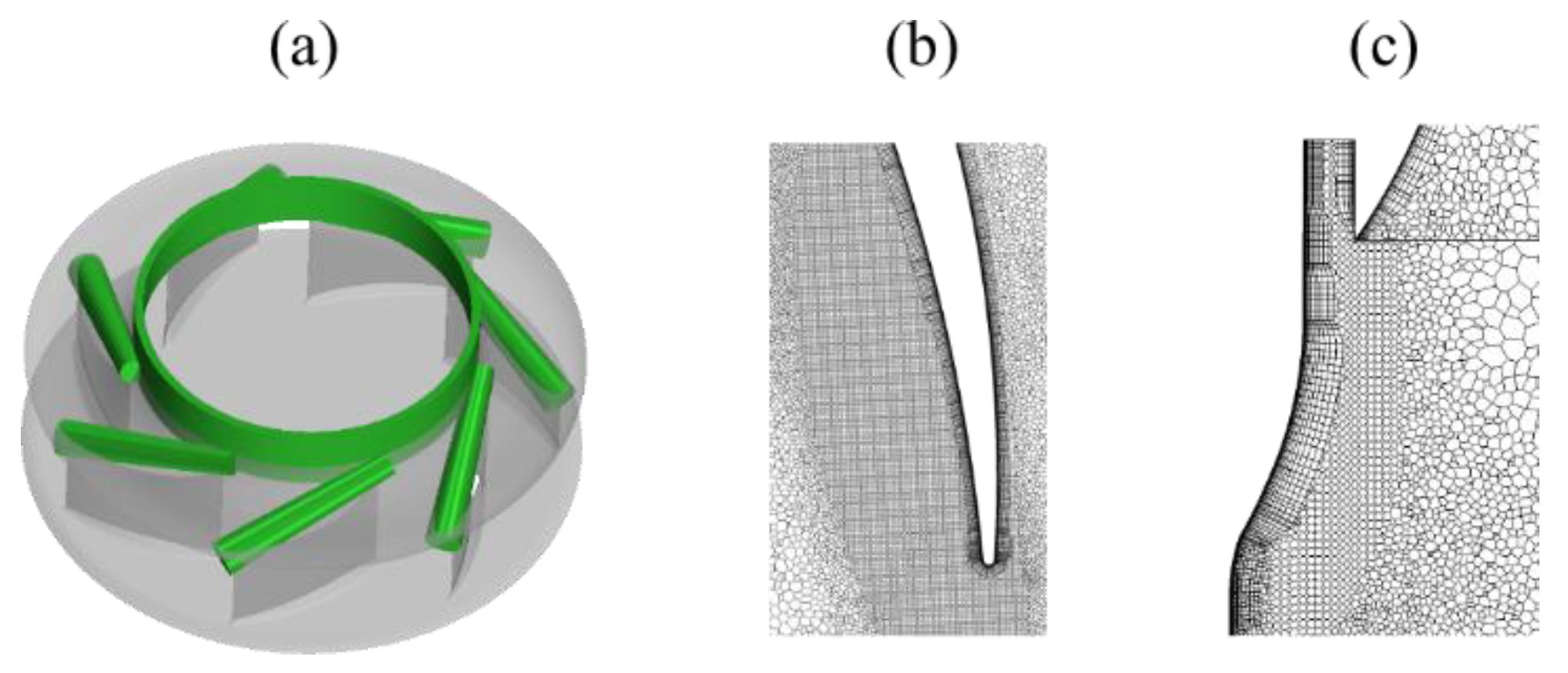
The entire computational domain is divided into stationary and rotating parts, corresponding to the regions within the ducts and fan, respectively. The mesh cells of the stationary and rotating parts are not conformable at the interfaces between the two parts.

The under-relaxation factors for the velocity and pressure are 0.7 and 0.4. The under-relaxation factor for the turbulence equations is 0.7.

A mass-flow rate boundary condition is set at the inlet, with a uniform velocity distribution. On the basis of $I=0.16{\left(R_e\right)}^{-1/8}$ [25], the modeled turbulence intensity is set to $I=4\%$. Here, $R_e$ is computed based on the inlet diameter ($d_3)$ and the streamwise velocity at the inlet. The modeled turbulence length scale is set to $\ell =0.5 \mathrm{m}$ based on $\ell =0.7d_3$ where $d_3$ is the inlet diameter. The pressure-outlet boundary condition is set at the outlet with the static pressure of 101,325 Pa, which is the reference pressure ($p_{ref}$) in the ambient air. The no-slip boundary condition is specified on all walls.

The time step is $\Delta t=2.0\times {10}^{-5} \mathrm{s}$. As a result, a maximum convective Courant number (CFL) of around 10 is obtained in the present simulations. In the previous studies [14,15], it has been proven that this time step gave almost the same results as the simulations with $CFL=1$ and the experiments. Since an implicit time-marching method is used in the present simulations, $CFL=10$ satisfies the requirement of the numerical stability, which has also been confirmed in the present simulations and the previous studies [14,15]. The maximum number of inner iterations per time step is set to 12.

As shown in Figure 3, three cut planes (Planes 1–3) across the fan are defined to monitor contours of the flow quantities. The results are discussed in the following sections.

4. CFD Mesh

The mesh generation strategy refers to [14], where the meshing has been validated for the same centrifugal fan. Polyhedral cells in the volume and prism layers near the walls are generated according to the recommendations on the meshing for turbomachines shown in [23,32]. The cell-size growth rate is set to 1.05 [33]. By following the meshing method in [14], the regions from the gap to the blade leading edge (BLE) and along the shroud to the blade trailing edge are refined. As shown in Figure 4, these mesh refinement regions are colored green. The mesh parameters are listed in

Table 2. The mesh parameters.

Total number of cells	$52\times {10}^6$
Number of cells in rotating zone	$41.9\times {10}^6$
Maximum first cell height $\Delta y^{+}$ near blade walls	0.73
Growth ratio of cell size	1.05

.

5. Results and Discussions

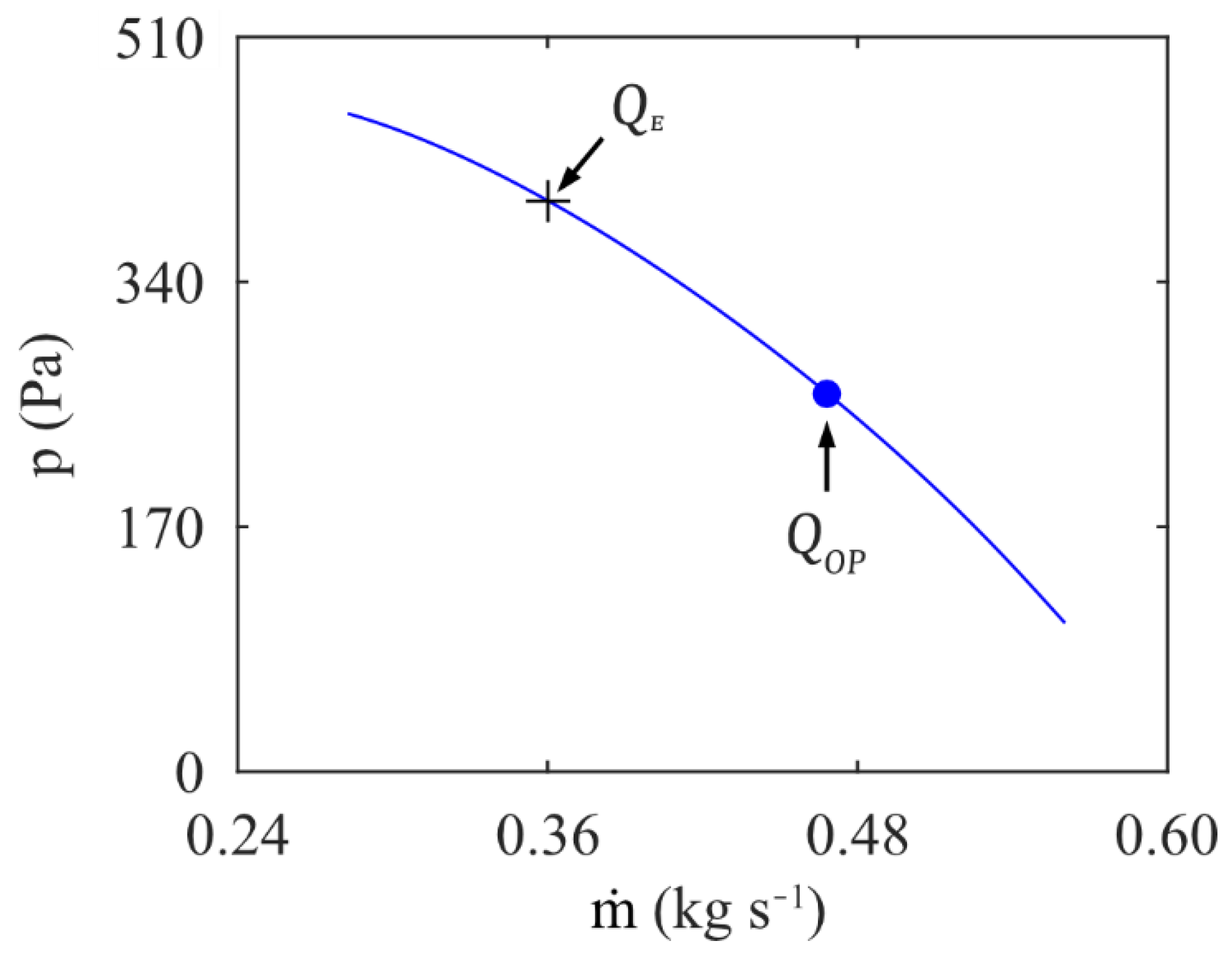
5.1. The Aerodynamic Performance of the Fan

The fan aerodynamic performance is analyzed in terms of the time-averaged static pressure rise between the fan inlet and outlet, $\Delta \overline{p}$, and the time-averaged fan torque $\overline{M}$. By setting the mass flow rate $\overline{Q}=0.36$ for the simulations, the results of these two quantities are listed in

Table 3. Time-averaged performance of the fan.

	$\Delta \overline{\mathit{p}} \left(\mathbf{Pa}\right)$	$\overline{\mathit{M}}$$(\mathbf{N}·\mathbf{m})$	$\overline{\mathit{Q}}$ (kg/s)
Simulation	267.8	1.127	0.36
Experiment	269.7	1.125	0.36

. They are in good agreement with the experimental data reported in the previous study [14].

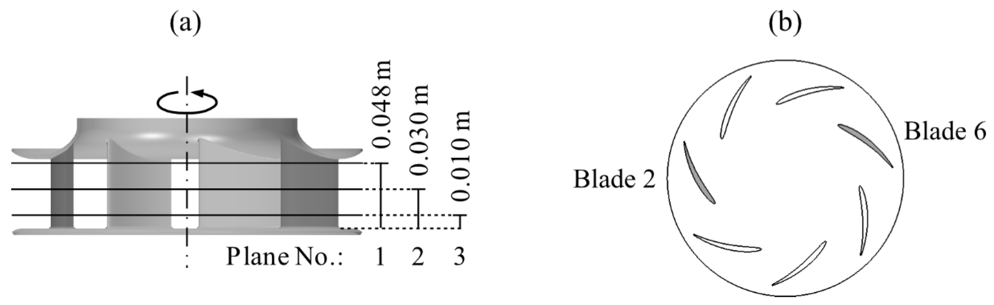
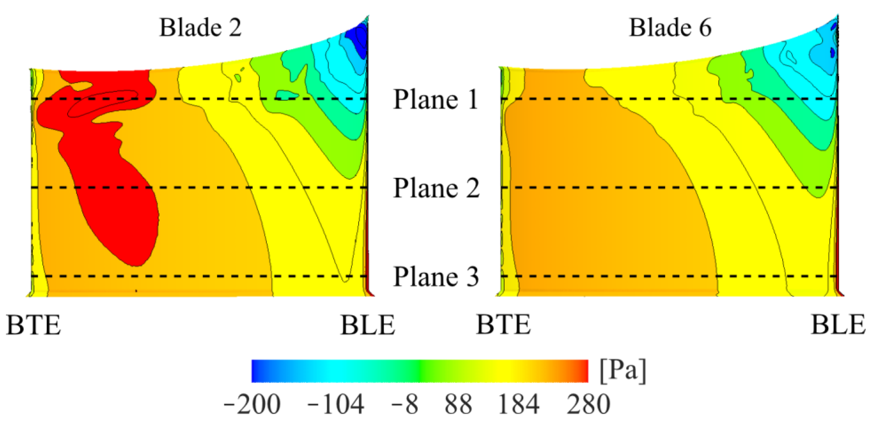
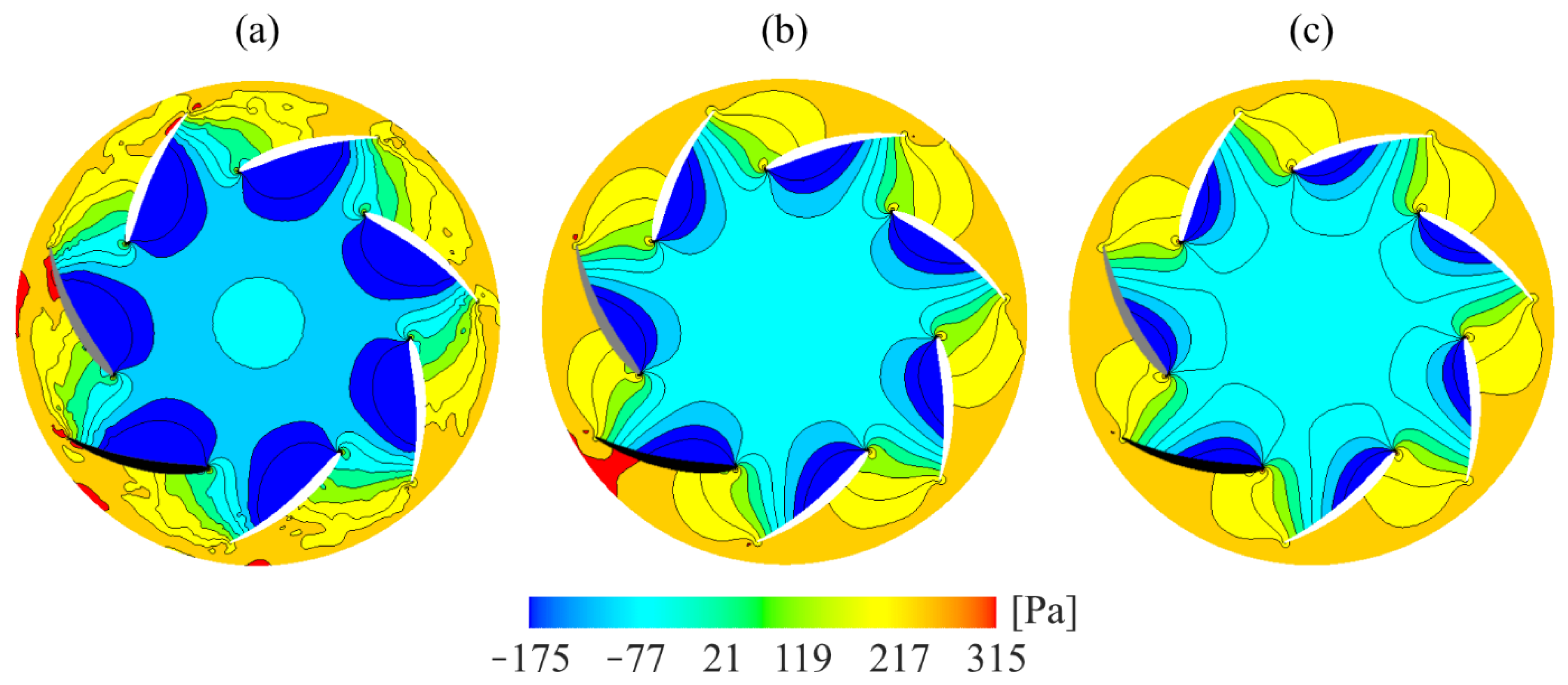
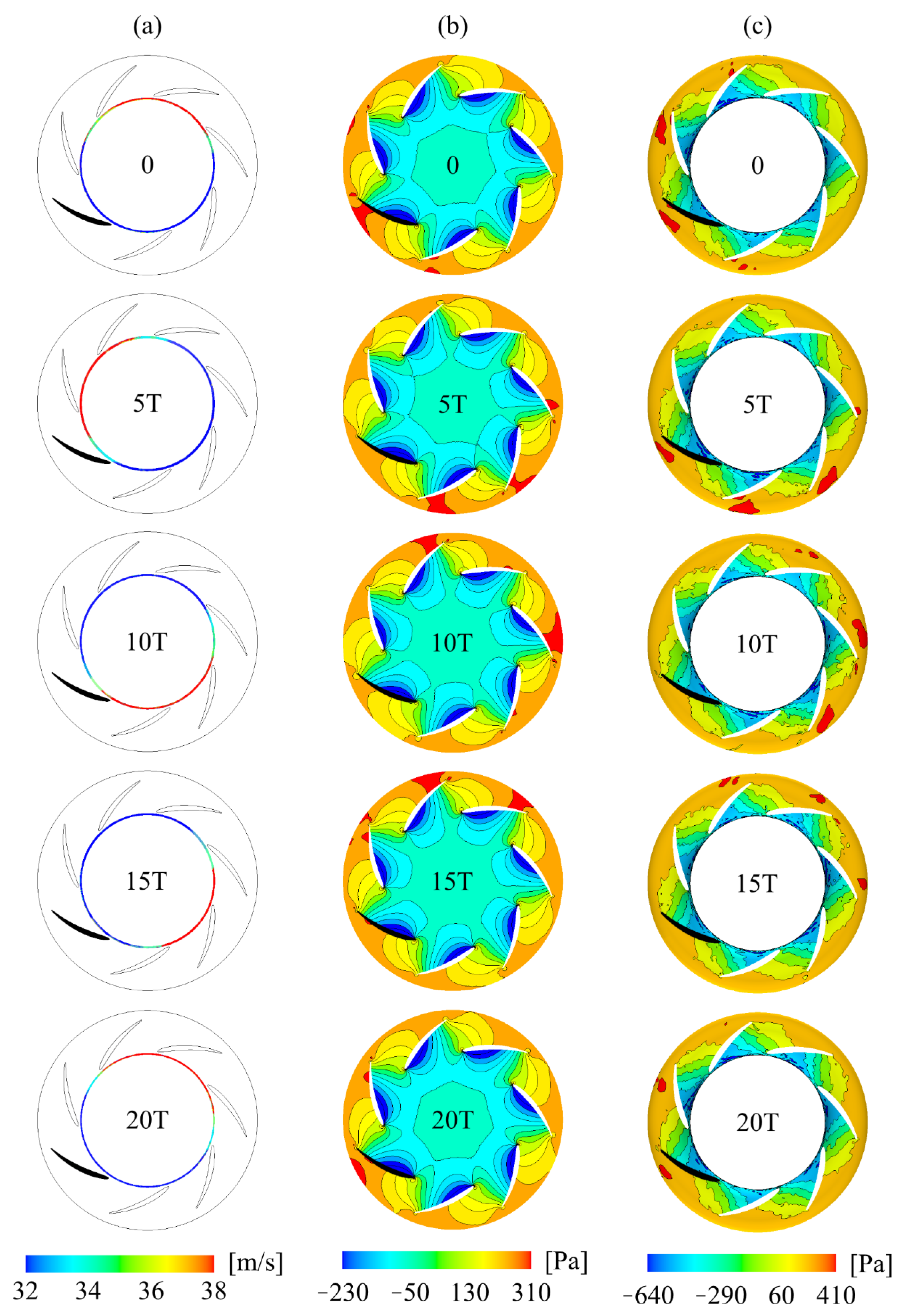
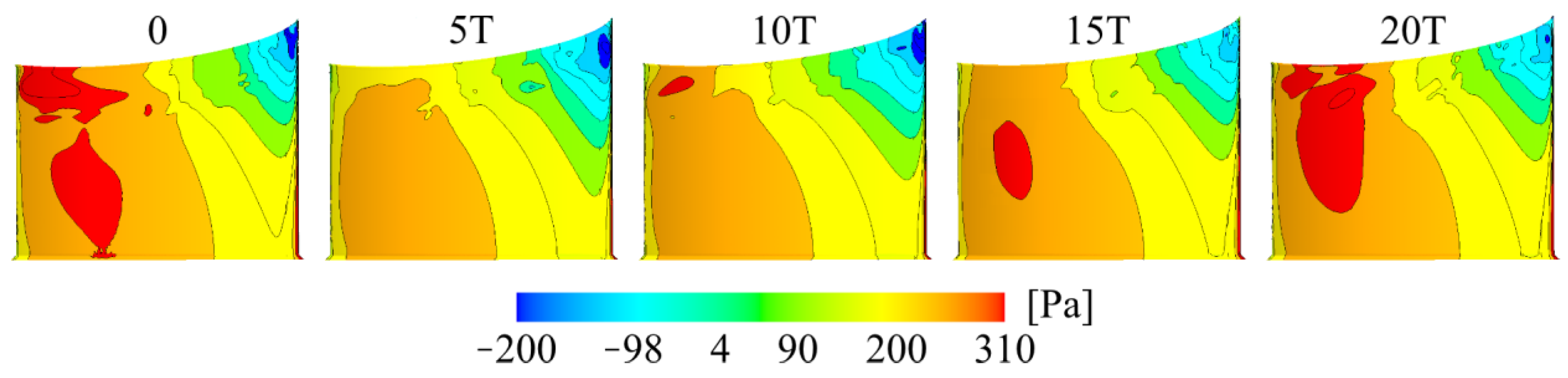
5.2. Unevenly Distributed Pressure and Velocity

Strong vorticity was found near the trailing edge of the blade, and it commenced periodically between the blades in [12]. To further address this effect, an arbitrary physical time is chosen to visualize the transient flow field. The iso-surfaces of the vorticity magnitude of $\Vert \overrightarrow{\omega }\Vert =8000 {\mathrm{s}}^{-1}$ near Blades 2 and 6 are shown in Figure 5. In addition, streamlines are displayed. The results are viewed from the pressure side of the blade. Blade 2 is viewed because it exhibits the largest turbulence at the chosen physical time. According to [12], the position of the largest turbulences will move to the other blades sequentially with a period. As a periodic effect, it can be discussed at an arbitrary snapshot. The iso-surfaces signify turbulent vortices from the gap, as found in [14]. There are more turbulent flow structures at Blade 2 that are swept along the intersection between the blade and shroud compared with Blade 6. Near Blade 6, turbulence is only noticed near the blade leading edge (BLE) and the blade trailing edge (BTE).

All velocities are shown in the rotating coordinate system. Velocity vectors near the pressure side of Blades 2 and 6 are presented in Figure 6. It can be seen that for Blade 6, the flow follows the blade profile. However, for Blade 2, the flow changes direction at a position close to the shroud near the BTE side.

For the convenience of the analysis, the static pressure is defined $p=P-p_{ref}$, where $p_{ref}=101325 \mathrm{Pa}$. The static pressure p on the surfaces of the pressure side of Blades 2 and 6 is displayed in Figure 7. There is a region with large pressure on Blade 2 near the BTE, which is at the same location as where the flow changed direction in Figure 6. Blade 6 has no region with high pressure at the BTE. Additionally, a region with low pressure at the BLE close to the shroud is found for Blade 2 but not for Blade 6. The same finding was presented in the previous numerical simulations for this fan [14]. In that study, it was concluded that the surface-pressure fluctuations at the BLE close to the shroud are responsible for the tonal noise at the $BPF$.

Figure 8 shows the instantaneous pressure, $p$, in Planes 1, 2, and 3 (see the plane positions in Figure 3 and Figure 7). Unevenly distributed pressure is found for Planes 1 and 2. In Plane 2, the pressure at the pressure side is highest at Blade 3 (colored black). In Plane 1, the pressure is highest at Blade 2 (colored gray), but small regions can also be found on blades 1 and 3. The pressure is almost the same for all blades at Plane 3, which is close to the backplate. The high-pressure regions decrease as the distance to the gap and shroud increases, and the pressure becomes evenly distributed among the blades. In a previous study of this fan [14], it was found that the uneven pressure distribution is connected to the turbulence in the blade passage generated by the flow through the gap.

A snapshot of isosurfaces of $p=340 Pa$ and contours of the velocity magnitudes at the gap is illustrated in Figure 9a. Note that in the fan passages, $340 Pa$ is comparatively high pressure. As seen in the figure, high pressure (colored in orange) only exists at the pressure side of Blades 2 and 3 close to the BTE. In the upstream locations of these blades, the velocity magnitudes are comparatively low.

To compare the local flow fields near Blades 2 and 6, Figure 9b shows the iso-surfaces of $p=340 Pa$, streamlines, and the velocity magnitudes at the gap entry. The high-pressure iso-surfaces are only observed near the BTE of Blade 2 but not Blade 6. These high-pressure regions are located downstream of the flow from the gap, and the streamlines are distorted near the regions. In contrast, the streamlines evolve smoothly near Blade 6. As can be seen from the figure, once the velocity magnitudes at the gap entry are low, the high-pressure regions appear near the BTE. This effect is generally observed during the fan rotation and is exemplified in the present snapshot. The turbulence initialized at the gap affects the flow at the blade and shroud intersection on the pressure side of the blades. In previous studies of this fan [14], it was concluded that turbulence initializes when the gap flow is mixed with the main flow and that the turbulence occurs unevenly among the blades. Note that the instantaneous flow quantities analyzed in this section are extracted at the same physical time.

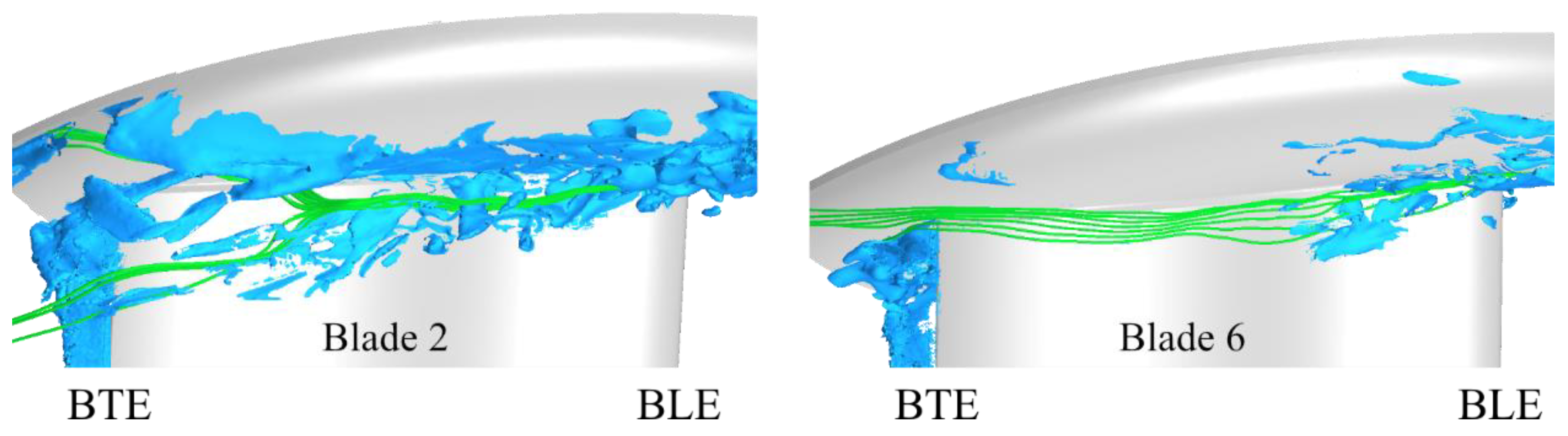
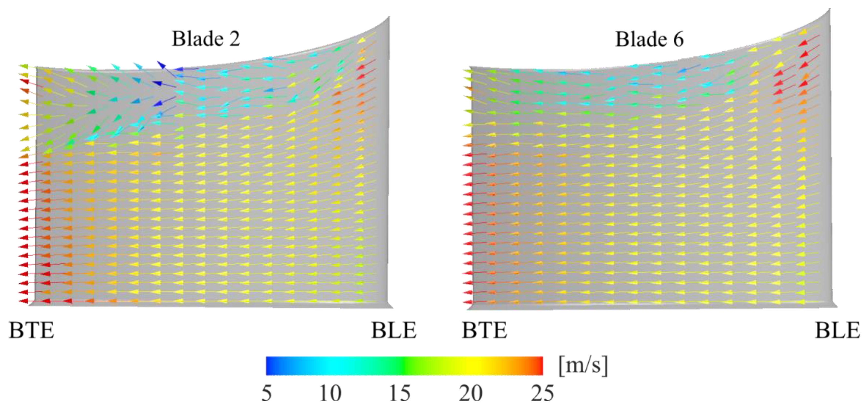
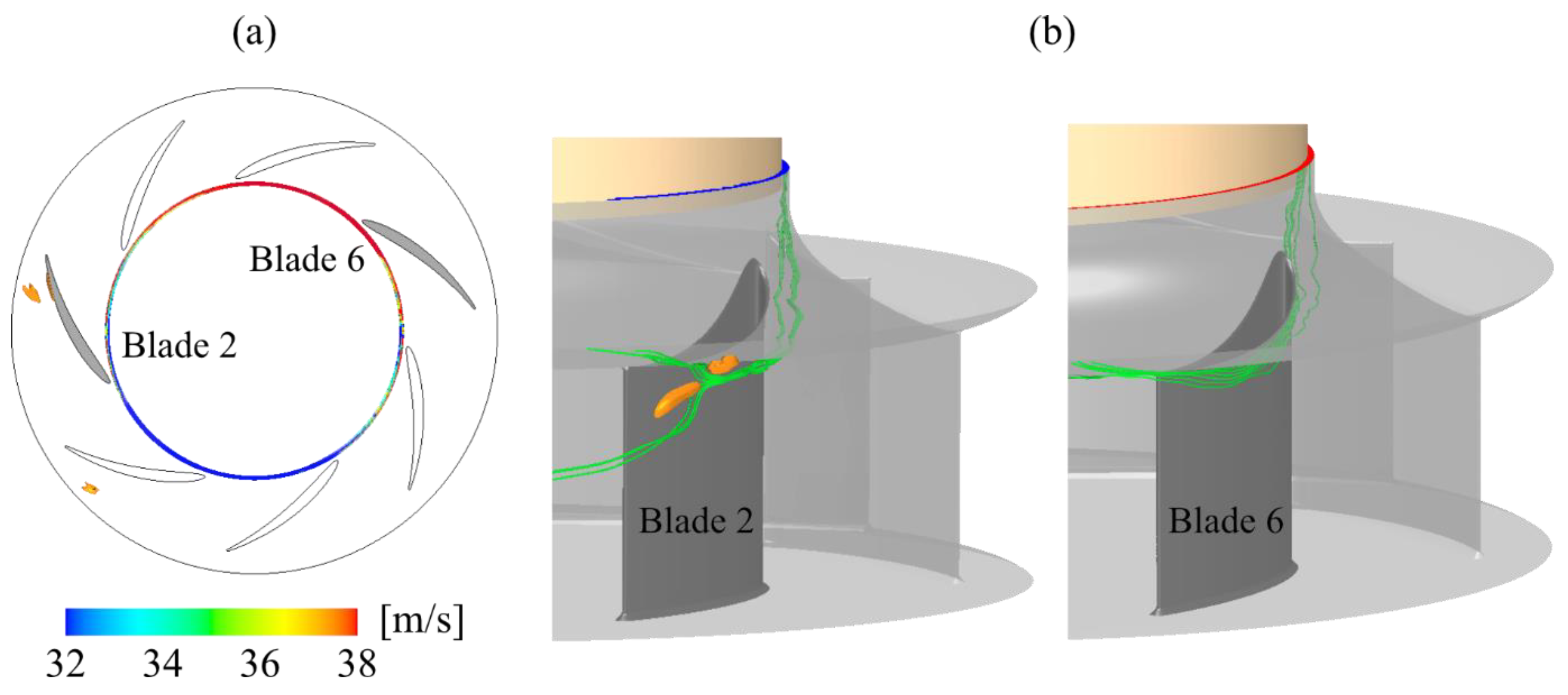
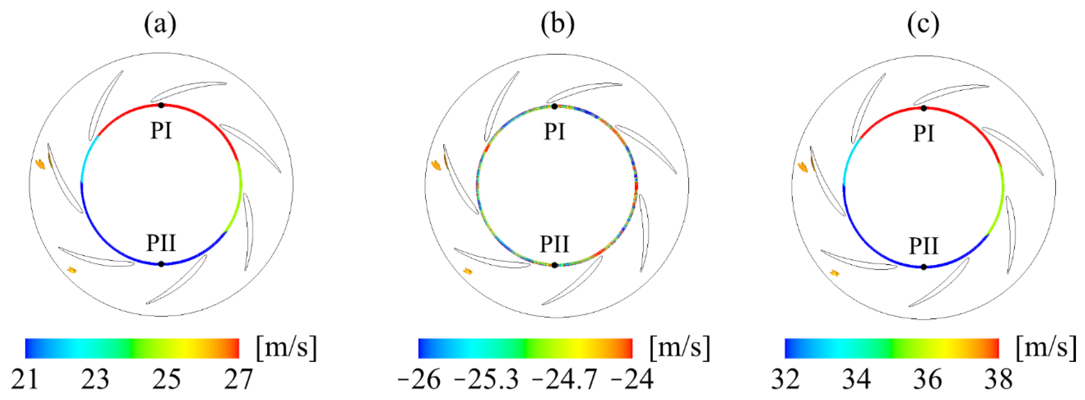
5.3. Velocities at the Gap

A snapshot of the contours of three different velocities at the gap and the iso-surface of $p=340 Pa$ is illustrated in Figure 10. The velocities are: (a) the tangential velocity, defined as $\left|v_T\right|=\sqrt{v_y^2+v_z^2}$, (b) the axial velocity, and (c) the velocity magnitudes (the coordinate axes defined in Figure 1). As can be seen, the tangential velocity and the velocity magnitudes are unevenly distributed at the gap. They are structured in obvious low- and high-velocity regions, and the two regions are located on opposite sides. In contrast, for the axial velocity, the low and high values are randomly scattered.

Since the high and low velocity appear on the opposite sides within the gap (see Figure 10), we set up two monitoring points (PI and PII) following the fan rotation in order to understand how the velocity varies over time. Figure 11 displays the time history of the tangential velocity, the axial velocity, and the velocity magnitude at PI and PII. The fan rotation period is $\mathrm{T}=0.0214 \mathrm{s}$. Over 25 fan periods (25T) are monitored. The tangential velocity has larger fluctuations compared to the axial velocity, and it is clear that it is responsible for the uneven velocity magnitudes at the gap.

In Figure 11, the fitting curves colored red are calculated using the smoothing function Gaussian with a smoothing factor of 0.4. A low-frequency wave can be seen for all three variables, especially for the tangential velocity and the velocity magnitudes. This indicates that the tangential velocity contains a fluctuation at a frequency that is much lower than the fan rotation speed. By comparing the low-frequency fluctuations of the tangential velocity at PI and PII, it is seen that the wavelengths between the two locations are the same, but the phase difference of the waves is about half their period. Since the axial velocity is much smaller than the tangential velocity, the total velocity magnitude also shows a similar trend to the tangential velocity.

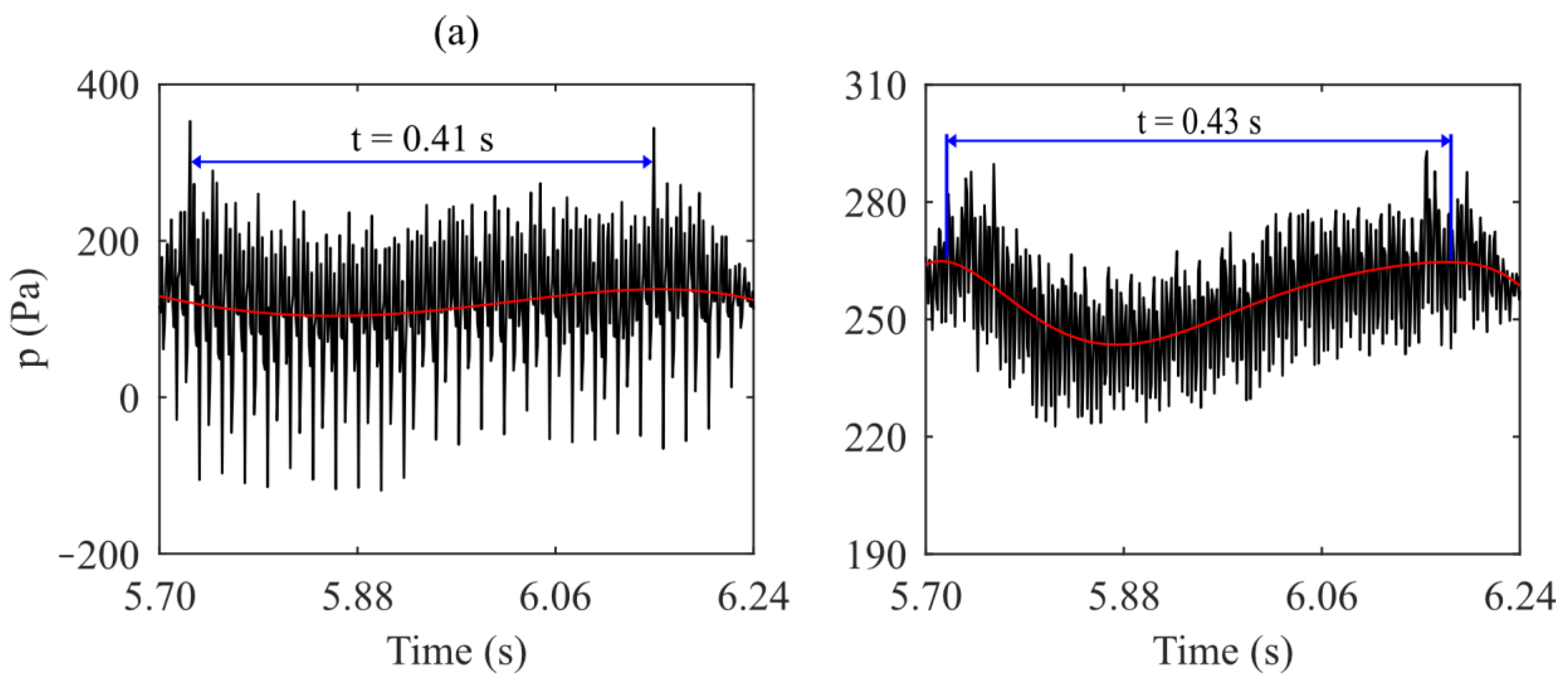
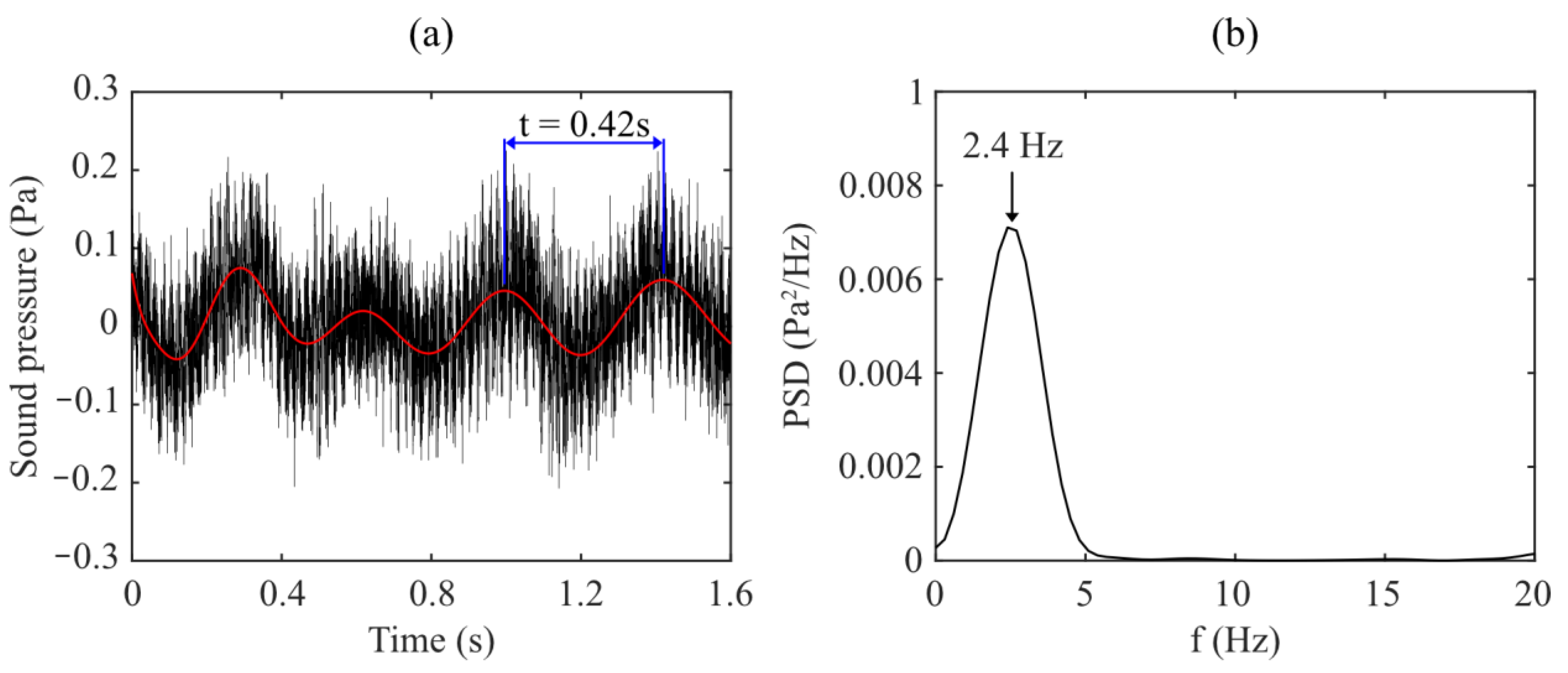
5.4. Low-Frequency Rotation

Two monitor points, P1 and P2, are set to observe pressure, as shown in Figure 12. P1 is located near the shroud and Blade 2, and P2 is located on Plane 2, i.e., approximately the midspan of the blades. The time history of the pressure p at these monitor points is displayed in Figure 13. The monitor points follow the fan rotation and the time history is shown over 25T. The curves are fitted with the Gaussian smoothing function in MATLAB with a smoothing factor of 0.4 and are colored in red. A low-frequency fluctuation is found (the same as shown in Figure 11), with a time period of $0.41 \mathrm{s}$. Additionally, in Figure 13b, a low-frequency fluctuation is found for the curve fit, with a time period of $0.41 \mathrm{s}$. These results indicate that a low-frequency rotation in relation to the fan rotation takes place in the fan and that the period time is approximately $0.42 \mathrm{s}=20\mathrm{T}$. This was also found in [14], but these studies provided few discussions on the physical mechanisms.

In previous studies of this fan [14,23], the aerodynamics and aeroacoustics were validated with experiments. The sound pressure measured near the inlet in the experimental rig is displayed in Figure 14. Additionally, here, a low-frequency rotation is observed, with a time period of $0.42 \mathrm{s}=20\mathrm{T}$. Moreover, the power spectral density (PSD) of the sound pressure is shown in Figure 13b. A tonal frequency of $2.4 \mathrm{Hz}$ is observed, which is consistent with the rotation period of $0.42 \mathrm{s}$ found in the experiments for this fan. This supports the conclusion in Figure 13. The low-frequency rotation period ($2.4 \mathrm{Hz}$) is much lower than the frequency of a rotating stall.

Figure 15 displays snapshots of the transient pressure $p$ in Plane 2, where $\mathrm{T}=0.0214 \mathrm{s}$ is the fan rotation period. The pressure is unevenly distributed. Blade 3 is colored black to indicate the blade position every 2.5T during 20T. The largest pressure region is observed to move amongst the blades sequentially. This region is seen at the same position, at $t_0$ and $t_0+20T$. Previous experimental studies [10,11] have observed the same physical behavior of high pressure and large TKE at the blade’s pressure side close to the BTE.

Figure 16 illustrates the transience of the velocity magnitudes at the gap and the transient pressure $p$ in Plane 2, and on the shroud. Here, Blade 3 is colored black to illustrate the fan rotation process. There are regions with low-velocity magnitudes at the gap and regions with high surface pressure on the shroud. The regions vary with the same angular speed as the high-pressure regions in Plane 2. Moreover, high-pressure regions always exist at the same circumferential position as the regions with low-velocity magnitudes. This phenomenon is explained in terms of the high turbulence regions and streamlines illustrated in Figure 5 and Figure 6. The flow through the gap causes turbulent flow structures, which are unevenly distributed among the blades. Regions with high pressure always occur at the blades where the flow is highly turbulent. It is concluded that the region of high pressure is connected to large turbulent structures triggered by the low-velocity region at the gap.

The transient pressure p on the pressure side surface of Blade 3 (colored black in Figure 15 and Figure 16) is displayed in Figure 17. Large pressure regions are observed to periodically occur among the blades. For example, such a region appears on Blade 3 at $t_0$ and $t_0+20T$, where $\mathrm{T}=0.0214 \mathrm{s}$ is one fan period. Therefore, one conclusion is that the revolution period of the high-pressure region on the blade surfaces is 20T. This supports the findings in Figure 13, Figure 14, Figure 15 and Figure 16.

6. Conclusions

The unsteady low-frequency characteristics are investigated for a voluteless centrifugal fan for HVAC systems. Given that the frequency is much smaller than the BPF (about 20 times the fan rotation period, as we find in this study), the flow simulation using IDDES is performed for an extremely physical time. This provokes a major challenge against the state of the art of the fan simulation, since IDDES has high computational costs and a very long computational time is needed to achieve the physical time.

At the gap entry, the velocity magnitudes are unevenly distributed, with clear low- and high-velocity regions. The tangential velocity component in the rotation direction of the fan plays a dominant role in this effect, whereas the velocity component in the fan axial direction is turbulent. An interrelation is found between the velocity at the gap entry and the pressure inside the fan. As the velocity magnitude is low, high pressure commences on the blade pressure side near the trailing edge. Turbulent vortices are significantly triggered from the low-velocity region at the gap entry and are swept along the intersection between the blade and shroud. Furthermore, the flow is distorted around the locations of the high pressure. However, this effect decays as the spanwise distance to the shroud increases. Relatively even pressure distribution is found near the fan backplate.

Unsteadiness with an ultralong period of 20T is identified for the fluctuating velocity at the gap entry and for the fluctuating high pressure inside the fan. Here, $\mathrm{T}=0.0214 \mathrm{s}$ is one fan rotation period. In previous acoustic measurements of this fan, tonal infrasound at 2.4 Hz was identified in the noise. This frequency is in line with the ultralong period of the flow unsteadiness. Therefore, it is deduced that the low-frequency unsteadiness from the gap entry is responsible for the tonal infrasound generation.

References

1. Roberts, T. We Spend 90% of Our Time Indoors. Says Who? 2016. Available online: https://www.buildinggreen.com/blog/we-spend-90-our-time-indoors-says-who (accessed on 20 June 2022).
2. Berglund, B.; Lindvall, T.; Schwela, D. New Guidelines for Community Noise. Noise Vib. Worldw. 2000, 31, 24–29. [Google Scholar] [CrossRef]
3. Azimi, M. Noise Reduction in Buildings Using Sound Absorbing Materials. J. Archit. Eng. Technol. 2017, 6, 198. [Google Scholar]
4. Seabi, J.; Cockcroft, K.; Goldschagg, P.; Greyling, M. A prospective follow-up study of the effects of chronic aircraft noise exposure on learners’ reading and comprehension in South Africa. J. Expo. Sci. Environ. Epidemiol. 2015, 25, 84–88. [Google Scholar] [CrossRef] [PubMed]
5. Klatte, M.; Bergstrom, K.; Lachmann, T. Does noise affect learning? A short review on noise effets on cognitive performance in children. Front. Psychol. 2013, 4, 578. [Google Scholar] [CrossRef] [Green Version]
6. Ffowcs Williams, J.E.; Hawkings, D.L. Theory relating to the noise of rotating machinery. J. Sound Vib. 1969, 10, 10–21. [Google Scholar] [CrossRef]
7. Lee, Y. Impact of fan gap flow on the centrifugal impeller aerodynamics. J. Fluids Eng. 2010, 132, 091103. [Google Scholar] [CrossRef]
8. Lee, Y.; Ahuja, V.; Hosangadi, A.; Birkbeck, R. Impeller Design of a Centrifugal Fan with Blade Optimization. Int. J. Rotating Mach. 2011, 2011, 1–16. [Google Scholar] [CrossRef] [Green Version]
9. Ottersten, M.; Yao, H.-D.; Davidson, L. Numerical and experimental study of tonal noise sources at the outlet of an isolated centrifugal fan. arXiv 2020, arXiv:2011.13645. [Google Scholar]
10. Ubaldi, M.; Zunino, P.; Cattanei, A. Relative Flow and Turbulence measurements Downstream of a Backward Centrifugal Impeller. J. Turbomach. 1992, 115, 543–551. [Google Scholar] [CrossRef]
11. Johnson, M.W.; Moore, J. The Development of wake flow in a Centrifugal Impeller. J. Eng. Power 1980, 102, 382–389. [Google Scholar] [CrossRef]
12. Pavesi, P.; Ardizzon, G.; Cavazzini, G. Experiments on the unsteady flow field and noise generation in a centrifugal pump impeller. J. Sound Vib. 2003, 263, 493–514. [Google Scholar]
13. Mongeau, L.; Thompson, D.; McLaughlin, D. Sound generation by rotating stall in centrifugal turbomachines. J. Sound Vib. 1993, 163, 1–30. [Google Scholar] [CrossRef]
14. Ottersten, M.; Yao, H.-D.; Davidson, L. Tonal noise of voluteless centrifugal fan generated by turbulence stemming from upstream inlet gap. Phys. Fluids 2021, 33, 075110. [Google Scholar] [CrossRef]
15. Ottersten, M.; Yao, H.-D.; Davidson, L. Inlet gap effect on aerodynamics and tonal noise generation of a voluteless centrifugal fan. J. Sound Vib. 2022, 540, 117304. [Google Scholar] [CrossRef]
16. Schwartz, S. Linking noise and vibration to sick building syndrome in office buildings. Air Waste Manag. Assoc. Mag. Environ. Manag. 2008, 3, 26–28. [Google Scholar]
17. Moënne-Loccoz, V.; Trébinjac, I.; Poujol, N.; Duquesne, P. Low frequency stall modes of a radial vaned diffuser flow. Mech. Ind. EDP Sci. 2019, 20, 805. [Google Scholar] [CrossRef]
18. Zheng, X.; Liu, A. Phenomenon and mechanism of two-regime-surge in a centrifugal compressor. J. Turbomach. 2015, 137, 081007. [Google Scholar] [CrossRef]
19. He, X.; Zheng, X. Flow instability evolution in high pressure ratio centrifugal compressor with vaned diffuser. Exp. Therm. Fluid Sci. 2018, 98, 719–730. [Google Scholar] [CrossRef]
20. Haynes, J.M.; Hendricks, G.J.; Epstein, A.H. Active stabilization of rotating stall in a three-stage axial compressor. ASME 1993; ASME Paper No. 93-GT-346. J. Turbomach. 1994, 116, 226–239. [Google Scholar] [CrossRef]
21. Paduano, J.D.; Greitzer, E.M.; Epstein, A.H. Compression system stability and active control. Annu. Rev. Fluid Mech. 2001, 33, 491–517. [Google Scholar] [CrossRef]
22. Tamaki, H. Study on flow fields in high specific speed centrifugal compressor with unpinched vaneless diffuser. J. Mech. Sci. Technol. 2013, 27, 1627–1633. [Google Scholar] [CrossRef]
23. Ottersten, M.; Yao, H.-D.; Davidson, L. Unsteady Simulation of tonal noise from isolated centrifugal fan. engrXiv 2020. [Google Scholar] [CrossRef]
24. Sanjose, M.; Moreau, S. Numerical simulations of a low-speed radial fan. Int. J. Eng. Syst. Model. Simul. 2012, 4, 47–58. [Google Scholar] [CrossRef]
25. Siemens PLM Software. STAR-CCM+ User Guide, Version 12.04; Siemens PLM Software: Plano, TX, USA, 2017. [Google Scholar]
26. Fitzpatrick, R. Chapter 1.6. In Theoretical Fluid Mechanics, Version: 20171201; IOP Publishing: London, UK, 2017. [Google Scholar]
27. Ferziger, J.H.; Peric, M. Computational Methods for Fluid Dynamics, 3rd ed.; Springer: Berlin, Germany, 2002. [Google Scholar]
28. Yao, H.-D.; Davidsson, L. Vibro-acoustics response of simplified glass window excited by the turbulent wake of a quarter-spherocylinder body. J. Acoust. Soc. Am. 2019, 146, 3163–3176. [Google Scholar] [CrossRef]
29. Shur, M.L.; Spalart, P.R.; Strelets, M.K.; Travin, A.K. A hybrid RANS-LES approach with delayed-DES and wall-modelled LES capabilities. Int. J. Heat Fluids Flow 2008, 29, 1638–1649. [Google Scholar] [CrossRef]
30. Rynell, A.; Efraimsson, G.; Chevalier, M.; Åbom, M. Inclusion of upstream turbulent inflow statistics to numerically acquire proper fan noise characteristics. SAE Tech. Pap. 2016, 1, 1811. [Google Scholar]
31. Rynell, A.; Chevalier, M.; Åbom, M.; Efraimsson, G. A numerical study of noise characteristics originating from a shrouded subsonic automotive fan. Appl. Acoust. 2018, 140, 110–121. [Google Scholar] [CrossRef]
32. Baris, O.; Mendonça, F. Automotive turbocharger compressor CFD and extension towards incorporating installation effects. In Proceedings of the ASME Turbo Expo 2011: Power for Land, Sea and Air, Vancouver, BC, USA, 6–10 June 2011. [Google Scholar]
33. Yao, H.-D.; Davidson, L.; Eriksson, L.E. Surface integral analogy approaches for predicting noise from 3D high-lift low-noise wings. Acta Mech. Sin. 2014, 30, 326–338. [Google Scholar] [CrossRef]
Figure 1. (a) The geometry setup of the numerical simulations. (b) The fan, stationary inlet duct, and gap between them. Red indicates the gap. The fan rotates about the x-axis.
Aerospace 09 00846 g001
Figure 2. The characteristic curve of the voluteless fan at the rotation speed of 2800   rpm . Q E is the mass flow rate at the maximum efficiency and Q O P is the mass flow rate at the operation point in this study.
Aerospace 09 00846 g002
Figure 3. (a) The cut planes for monitoring contours of the flow quantities. (b) The blades (in gray) followed to observe periodic evolutions of the transient flow field.
Aerospace 09 00846 g003
Figure 4. (a) The mesh refinement regions, colored green. Volume mesh cells near: (b) the blade trailing edge and (c) the inlet gap.
Aerospace 09 00846 g004
Figure 5. Iso-surfaces of the vorticity magnitudes at ω = 8000   s 1 (colored blue) and streamlines (colored green) emanating from the gap, being swept from the blade leading edge (BLE) to the blade trailing edge (BTE).
Aerospace 09 00846 g005
Figure 6. Velocity vectors close to the pressure side of Blades 2 and 6, colored with velocity magnitudes.
Aerospace 09 00846 g006
Figure 7. A snapshot of the transient pressure p on the surfaces of the pressure sides of Blades 2 and 6. is the sides of the blade trailing edge (BTE) and the blade leading edge (BLE) are marked out.
Aerospace 09 00846 g007
Figure 8. The instantaneous pressure p in (a) Plane 1, (b) Plane 2, and (c) Plane 3. Blade 2 is colored gray and Blade 3 is colored black.
Aerospace 09 00846 g008
Figure 9. Iso-surface of p = 340   P a colored in orange, and contours of (a) the velocity magnitudes at the entry of the gap. (b) Streamlines from the gap at Blades 2 and 6, and contours of the velocity magnitudes at the entry of the gap.
Aerospace 09 00846 g009
Figure 10. Transient iso-surfaces of p = 340   P a (colored orange) and transient velocities at the gap: (a) tangential velocity, | v T | , (b) axial velocity, and (c) velocity magnitudes. PI and PII show the locations of the monitor points placed in the gap.
Aerospace 09 00846 g010
Figure 11. The time history of the variables at the gap: of (a) the tangential velocity, | v T | , (b) the axial velocity, and (c) the velocity magnitudes. Black and gray lines: the instantaneous velocity; red lines: the fitted curves based on the Gaussian functions, the solid red line for Point I and the dashed red line for Point II.
Aerospace 09 00846 g011
Figure 12. Monitor points P1 and P2. The instantaneous pressure in Plane 2 and the iso-surface of p = 340   P a colored orange.
Aerospace 09 00846 g012
Figure 13. The time history of the pressure p in the monitor points, (a) P1 and (b) P2. The red lines are curve fits to the instantaneous pressure.
Aerospace 09 00846 g013
Figure 14. (a) The time history of the sound pressure from experimental results. (b) The PSD of the sound pressure at the microphone M1 upstream of the fan.
Aerospace 09 00846 g014
Figure 15. Snapshots of the transient pressure p in Plane 2. Blade 3 is colored in black.
Aerospace 09 00846 g015
Figure 16. Snapshots of: (a) the velocity magnitudes within the gap, (b) the pressure in Plane 2, and (c) the pressure on the shroud surface. To indicate the fan rotation process, Blade 3 is colored black.
Aerospace 09 00846 g016
Figure 17. Snapshots of the surface pressure p on Blade 3.
Aerospace 09 00846 g017