Abstract
UAS-based commercial services such as urban parcel delivery are expected to grow in the upcoming years and may lead to a large volume of UAS operations in urban areas. These flights may pose safety risks to persons and property on the ground, which are referred to as third-party risks. Path-planning methods have been developed to generate a nominal flight path for each UAS flight that poses relative low third-party risks by passing over less risky areas, e.g., areas with low-density unsheltered populations. However, it is not clear if risk minimization per flight works well in a commercial UAS operation that involves a large number of annual flights in an urban area. Recently, it has been shown that when using shortest flight path planning, a UAS-based parcel delivery service in an urban area can lead to society-critical third-party risk levels. The aim of this paper is to evaluate the mitigating effect of state-of-the-art risk-aware path planning on these society-critical third-party risk levels. To accomplish this, a third-party risk simulation using the shortest paths is extended with a state-of-the-art risk-aware path-planning method, and the societal effects on third-party risk levels have been assessed and compared to those obtained using shortest paths. The results show that state-of-the-art risk-aware path planning can reduce the total number of fatalities in an area, but at the cost of a critical increase in safety risks for persons living in areas that are favored by a state-of-the-art risk-aware path-planning method.
1. Introduction
Unmanned Aircraft Systems (UASs) [1] provide new opportunities for commercial services. UAS can be deployed for a large variety of commercial services, such as parcel delivery and urban air mobility. Although the number of UAS operations is not large as of yet, the global market for UAS-based commercial services is expected to increase to tens of billions of USD in the early 2030s (estimated by McKinsey [2]) and around 1 trillion USD by 2040 (estimated by Morgan Stanley [3]) Therefore, it is expected that there will be a large future volume of UAS operations in urban areas. However, these UAS operations pose safety risks to persons on the ground, referred to as Third-Party Risk (TPR). TPR posed by commercial UAS operations should be sufficiently mitigated such that the remaining risk levels are acceptably safe from a societal perspective.
Risk-aware path-planning methods in the literature developed as important means for mitigating safety risks posed by UAS flights to people on the ground. The key difference with shortest-path planning is that the safety risk is accounted for in the cost to be minimized. Path planning generates a set of waypoints that an unmanned aircraft (UA) should follow to reach a destination [4]. The planning minimizes the cost function that is associated with each possible path. The commonly used path-planning methods include graph-based and sampling-based methods. Graph-based algorithms search over the graph to find a path that has the minimum cost, such as Dijkstra’s algorithm [5]: A* [6] and its variants [7,8]. Two prominent types of sampling-based algorithms include the probabilistic roadmap method (PRM) [9] and rapidly exploring random tree (RRT) [10,11]. The PRM samples and connects points in the environment to construct a roadmap; then, it searches for a feasible path using the roadmap. RRT grows a unidirectional search tree from the starting point until a tree branch hits the goal point.
UAS risk-aware path-planning methods take into account the risk posed to people on the ground by a UA flight. They use risk maps to quantify the risk of flying over each position for each drone [12]. Risk analyses are invoked to evaluate the risk to people on the ground beforehand. A path with the minimum risk will be extended based on the risk map, e.g., riskA* [13,14] and risk-aware RRT* [15,16]. A bi-objective optimization is also used to minimize the trade-off between safety risk and flight distance [17]. Risk-based RRT* [18] does not use the risk-based map to estimate the risk; it directly computes the risk with risk assessment methods during planning paths. The UAS risk-aware path-planning method efficiently reduces the risk per flight by finding paths over areas with a low density of unsheltered populations.
Safety risks posed by a single UAS flight to the ground population has been well studied [19,20,21,22]. The common finding is that the risk posed per UAS flight hour to ground populations should be at an Equivalent Level Of Safety (ELOS) than the TPR posed per flight hour by a commercial aircraft, e.g. Clothier and Walker (2006) [22]. In commercial aviation, almost all fatalities concern crew and passengers onboard aircraft. This explains why the ELOS reference of the expected number of ground fatalities per flight hour is not a widely used TPR indicator in commercial aviation. Instead, TPR indicators are defined in terms of the safety risk posed to ground populations by all annual flights around an airport [23,24]. For these society-directed annual TPR indicators, models have been developed that allow assessments of changes in the risk posed to persons on the ground due to changes in the amount of flights, new departure/arrival routes, the impact of a new airport, the risk of constructing a residential building in a certain area, etc. Because similar annual TPR indicators are in use for hazardous facilities [24,25,26,27,28,29], there is ample experience in setting acceptable thresholds on these annual TPR indicators. This motivated Blom et al. (2021) [30] to extend the annual TPR indicators from conventional aviation to similar versions for UAS operations. In addition, existing TPR simulation models of UAS operations [31,32,33] have been extended for the assessment of these annual TPR indicators.
Blom et al. (2021) [30] have also conducted a simulation-based comparison of the ELOS-based TPR indicator and the annual TPR indicators for a hypothetical UAS-based parcel delivery service in the city of Delft by using the shortest flight paths. The simulation results obtained for this hypothetical example show that, in comparison to the ELOS indicator, the annual TPR indicators tend to pose higher safety mitigation needs on commercial UAS operations over urban areas. The objective of the current paper is to assess and compare the risk-mitigating effect of risk-aware path planning in terms of the ELOS-based and annual TPR indicators.
This paper is organized as follows. Section 2 reviews ELOS-based and annual TPR indicators applied in this paper, together with an explanation of the use of these TPR indicators within state-of-the-art UAS risk-aware path planning. The ELOS-based TPR indicator is the Collective Ground Risk per flight hour (CGRfh). The annual TPR indicators include the Annual Collective Ground Risk (CGR) and Annual Individual Risk (IR) map for each location in the urban area, posed by all UAS flights. Section 3 introduces the simulation methodology used for the evaluation of risk-mitigating effects of risk-aware path planning on the three TPR indicators for the parcel delivery service example in Delft. This includes an explanation on how risk-aware UAS path-planning algorithms are incorporated in the simulation. Section 4 conducts the simulation study of this paper for a commercial UAS-based parcel delivery service in the city of Delft that has been evaluated by Blom et al. (2021) [30] under the shortest paths. These results show the effect of risk-aware path planning on ELOS-based and annual TPR indicators. Section 5 discusses the obtained results. Section 6 draws conclusions.
2. Third-Party Risk Indicators and Path Planning
In this paper, three TPR indicators are involved: collective ground risk per flight hour (CGRfh), annual individual risk (Annual IR), and annual collective ground risk (Annual CGR). To allow a proper comparison of these three TPR indicators, this section reviews their formal definitions and explains their use in state-of-art path planning.
2.1. Third-Party Risk Indicators
Safety risks posed by a UAS flight to persons on the ground has been well studied [19,20,22,34] from the perspective that a single UAS flight should be allowed to pose an Equivalent Level Of Safety (ELOS) per flight hour to ground populations as is posed by a single commercial flight per hour. This level of safety is expressed in terms of the collective ground risk per flight hour (CGRfh). For the formal definition of CGRfh, Blom et al. (2021) [30] make use of an auxiliary definition of the collective ground risk per flight (CGRf): CGRf is the expected number of third-party fatalities on the ground per flight in a given area Y due to the direct consequences of a UA flight accident. Let be the number of third-party fatalities on the ground due to the i-th UA flight accident; then, the calculation of CGRf is as follows:
where is the fatality probability for an unprotected person at location y posed by the i-th flight, is the shelter protection model, and is the population density in the area Y considered. The characterization of in the UAS literature [12,30,31,35] satisfies the following:
where is the ground crash probability, is the crash location model, is the set of crash impact areas, and is the size of the crash impact area. is the unprotected fatality model. The CGRf considers the risk for a single flight. Let be the flight time for flight i; then, the collective ground risk per flight hour (CGRfh) for flight i is . It is a common practice to require that CGRfh for a UAS should not be higher than an Equivalent Level Of Safety (ELOS) of the CGRfh posed by a commercial aircraft flight to population on the ground.
The annual individual risk (Annual IR) [30] is the probability that an average unprotected person at ground location y gets killed or becomes fatally injured due to unmanned aircraft flight accidents during a given annum. This risk indicator considers the risk from multiple flight perspectives. For conducting N flights per annum, the annual IR is described as follows.
Often, ; then, Equation (3) can be approximated by . The safety threshold for the annual IR in the literature [27,29] indicates that the probability of fatality per annum at each location should not exceed .
Annual collective ground risk (Annual CGR) [30] is the expected number of third-party fatalities on the ground in a given area Y due to the direct consequences of ground crashes by unmanned aircraft flights during a given annum. This risk indicator considers the risk from the multiple flights perspective, i.e., flights in an annum. For conducting N flights per annum, the annual CGR is as follows:
where is defined in Equation (1). The annual CGR should not exceed 1.65 × 10 fatalities per annum [27,29]. The summary for the above indicators is shown in Table 1.

Table 1.
Summary for TPR indicators CGRfh, annual IR, and annual CGR.
2.2. TPR Indicators in Path-Planning
Existing risk-aware path planning methods use the indicator Collective Ground Risk per flight (CGRf) in searching for a nominal path for a given UAS flight from a point to a point . Optimization tools are used to minimize total cost function . For shortest-path planning methods, the total cost g is described as follows.
Here, is the flight distance of the nominal path.
Risk-aware path-planning methods take the cost of risks into account. If the goal is only the minimization of risk [13,14], then the cost g adopted is described as follows:
where is the accumulated collective ground risk (e.g., number of fatalities) on the flight path from point to per flight, which is basically CGRf. Under bi-objective optimizations [17,36], the total cost, g, considers both risks and flight distances.
The risk-to-distance ratio determines to which extend the found path detours high-risk areas.
There are two methods to evaluate as a function of the nominal path during the optimization process. One is to use the pre-defined risk map [12]. For each location on the map, the risk is pre-calculated based on static information (e.g., sheltering factor, population density, etc.). The other one is a sampling-based method [18] that iteratively samples a path from to and calculates the correlated risk.
An open question is how these three path-optimization methods (path length only, risk-aware only, and bi-objective) compare in terms of the annual safety indicators: annual IR and annual CGR. Such a comparison is made in Section 4 for a commercial parcel delivery service in the city of Delft. Prior to conducting these comparisons in Section 4, Section 3 gives an explanation on the method used to conduct these annual risk assessments.
3. Assessment of Annual Third-Party Risks for a Commercial UAS Service
A method to assess third-party risks posed to the ground population by a commercial UAS service has been developed by Blom et al. (2021) [30]. This method can handle an arbitrary large number N of annual origin-destination UAS flights. To take various disturbances into account, for each of these N UAS flights, a number of K independent Monte Carlo simulation runs are conducted. The sequence of steps to be conducted in this method is shown in Algorithm 1. Step 0–1 generates UA flight demands (OD pairs), and for each OD pair, there is a nominal flight path. Step 2 uses an applicable failure model to evaluate ground crash probabilities. Step 3 uses, for each type of failure, an applicable descent model to simulate the random descent path until the ground crash. Step 4 evaluates the distribution of the simulated ground crash locations. Step 5 uses an applicable human fatality risk model under the assumption that persons on the ground are unprotected. Step 6 assesses an individual risk map for each of the N UAS flights. Step 7–9 assess CGRfh, annual IR, and annual CGR, respectively.
| Algorithm 1: Monte Carlo simulation-based evaluation of annual Third-Party Risk indicators for a commercial UAS operation [30]. |
 |
In [30], the workings of this Monte Carlo simulation approach have been applied to a commercial UAS parcel delivery service in the city of Delft. The map of the city’s population is given in Figure 1. In [30], the nominal paths in the example application were the shortest distance paths. In the next subsection, an explanation is provided on how this is extended to single- and bi-objective risk-aware path planning in step 1 of Algorithm 1. The grid size of the possible OD pairs generated during Step 0 increased from 5 m in [30] to 500 m in Section 3.1. The specific details of Step 0 and Step 1 are described in Section 3.1 and Section 3.2, respectively.
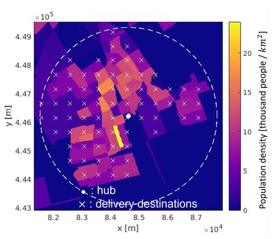
Figure 1.
Generated OD pairs (hub-delivery destinations) in the scenario.
3.1. Generation of N OD Pairs (Step 0)
During Step 0 of Algorithm 1, the annual flight demand is generated, including the number of OD pairs, the locations of OD pairs, and the number of flights for each OD pair. It assumes that the drone route’s network is from one hub to serve multiple delivery destinations inside a service radius.
The generation of OD pairs is based on population distributions. Recently, several studies looked at the forcast of air delivery/mobility demand distributions, and many factors are considered, e.g., population distributions, historical travel/delivery demands, residents’ incomes, different points of interest (POI), etc. [37,38,39]. In this study, for the sake of simplicity, we use the assumption in [30] in which the density of the parcel delivery location is the same as the population density within the service radius. The geographic map is discretized into multiple rectangular grid areas, and in each grid, if the average population density is beyond a threshold, the center of the grid will be selected as a destination. The simulations use an area in Delft, as shown in Figure 1. The width and length for the area are km and km separately, and the total size is 43.6 km. The population in the area is around 130,000 people. In the simulations, we take the service radius as km, the size of each grid as 0.5 km × 0.5 km, and the population density threshold as 2000 people/km. As a result, a total of 71 OD pairs are generated, as shown in Figure 1.
To estimate the number of UA flights per annum, more specifically, the number of flights for each OD pair per annum, we first estimate the number of package deliveries per person per annum. For example, if each person receives 10 package per year in Delft, then around 1.3 million packages are delivered in the above area in Delft, in which there are 130 thousand people. More specifically, if each person is served n packages in a year, the number of flights N from the hub to each delivery location is described as follows:
where is the number of people in the area covered by the delivery location.
3.2. Nominal Flight Path Generation (Step 1)
In Step 1 of Algorithm 1, nominal paths are determined for UA flights by a typical risk-aware path-planning algorithm.
We used an A*-based graph search method to represent typical risk-aware path-planning algorithms. The A*-based graph search method uses Equation (7) to search for a path. For the sake of simplicity, we use population density as the pre-defined risk at each location and sum population density over a path. and are the weights for the risk and the path length in Equation (7). We define the risk weight ratio as follows.
reflects how the risk and flight distance will be optimized. If is much larger than , e.g., 1:0, the total cost only includes . The generated path completely detours over low-populated areas, as shown in Figure 2a, so the path can have a low CGRf. If is much larger than , e.g., 0:1, the total cost only includes . The algorithm will search a short path, as shown in Figure 2b. By changing the risk weight ratio, the algorithm can generate different paths either by detouring over low-populated areas or by being short.
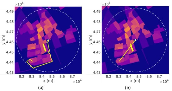
Figure 2.
An example of generated paths by setting (a) 1:0: a path over low-populated areas; (b) 0:1: a short path.
3.3. Risk Assessment via Monte Carlo Simulation
In conducting Steps 2–9 of Algorithm 1, specific submodels for UAS types, UAS failures, UAS descent path to ground crash, UAS crash impact area, and human fatality models have to be adopted. Their relationship is shown in Figure 3. For the Monte Carlo simulations conducted in Section 4, we adopt the same submodels that have been adopted by Blom et al. (2021) [30] for the Delft parcel delivery example.
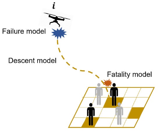
Figure 3.
The failure model, descent model, and fatality model in risk assessments.
In the UAS parcel delivery example used in [30], the hypothetical drones are based on the MD4-1000 quadcopter from Microdrones [40]; each drone has a mass of 2.7 kg and the payload is up to 1 kg. Moreover, the surface area of drones is 0.1 m. The full list of parameter values is stated below. The cruise, ascent, and descent speeds are 12, 7.5, and 6 m/s, respectively [41]. Horizontal and vertical position errors follow Gaussian distributions, and the standard deviations are 3.68 m and 7.65 m, respectively [42]. Standard deviations for horizontal and vertical velocity errors are both 2.0 m/s [43]. The drag coefficient of drones follows a Gaussian distribution [43]. The summary of these parameters is provided in Table A1.
The failure model describes the probability that an in-flight failure happens. Let be the rate of a crash event happens at moment t during the ith flight, and the nominal flight time of i-th flight is . Then, the probability of a crash is described as follows.
A constant is used in the MC simulation.
The descent model describes how a drone descends to the ground after an in-flight failure happens. A ballistic descent model [12] is used in the MC simulation to estimate the crash location. In this model, the descending crash is affected by the drag coefficient and the surface area of the drone, in addition to wind velocities. Let and represent the position and velocity of the drone at time t; then, the ballistic descent model is described as follows:
where g is the gravitational constant, is the drag coefficient, is the size of surface area, m is the mass of the drone with payload, and and are air density and wind velocity vectors at time t.
The fatality model describes the fatality probability for different impact energies. A commonly used fatality model [44] is applied in the MC simulation. It is an S-shaped curve:
where Z is the cumulative standard normal distribution, is the kinetic energy of an unmanned aircraft at the moment of impact, with impact velocity v and with impact mass m, a is the energy when the probability of fatality reaches 1/2, b is the standard deviation of the effect of . The parameters a and b reflects the fatality probability of an object hitting a person. In the experiment we take the fitted value Joule and [45], the curve of the fatality model is shown in Figure 4.
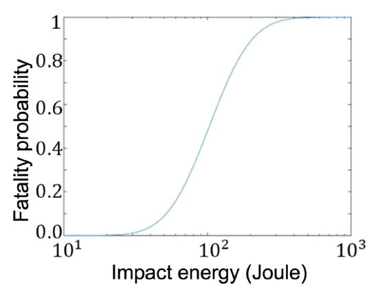
Figure 4.
The RCC fatality model with parameters Joule and .
4. Simulation Results
We conducted three experiments and analyses based on the assessment in Section 3. Experiment I tests how annual third-party risks changes as path-planning objective changes; i.e., the risk weight ratio in path planning increases. Experiment II tests how annual TPRs change with the volume of flight operations, and experiment III conducts sensitivity analyses: it tests how annual TPRs are sensitive to risk assessment parameters.
4.1. Experiment I: Risk Weight Ratio
This experiment simulates whether the current path-planning algorithm can reduce annual TPR by changing the risk weight ratio in the path-planning algorithm. Here, the flight volume is set as 1 package per person per annum.
Here, we evaluate different weights where the risk weight ratio increases gradually. The generated paths are shown in Figure 5. When the weight ratio on risk is higher, paths detour to lower populated areas, and flight distances are longer.
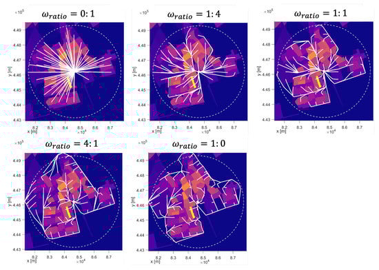
Figure 5.
Generated paths with different risk weight ratios.
The histograms of CGRfh are shown in Figure A1 in Appendix A. All flights have CGRfh at an acceptable level (<10 fatalities per flight hour). As the risk weight ratio increases, the maximum CGRfh reduces from 5.34 × 10 per flight hour to 2.58 × 10 per flight hour, and the mean value also reduces from 2.72 × 10 per flight hour to 6.12 × 10 per flight hour.
The annual IRs over the map are shown in Figure 6. Bright yellow and orange colors mean higher annual IR and dark purple means a lower annual IR. As the risk weight ratio increases, more areas are colored orange instead of purple in Figure 6 intuitively, meaning that more areas have high annual IRs. The precise area size of high annual IRs ([30]) is shown in Table 2, which increases from 0.75 km to 2.47 km.
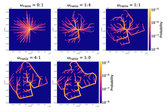
Figure 6.
Annual IR with different risk weight ratios.
Table 2.
Area size with high annual IR with different risk weight ratios.
The annual CGR is shown in Table 3. The annual CGR reduces from 3.00 × 10 fatalities per annum to 1.57 × 10 fatalities per annum as the risk weight ratio increases. Under the threshold of 1.65 × 10 fatalities per annum, only can generate paths that satisfy the annual CGR criterion.
Table 3.
Annual CGR with different risk weight ratios.
The relationship between annual TPRs (annual IR and annual CGR) and risk weight ratio is shown in Figure 7. As the risk weight ratio increases, annual IR increases but the annual CGR reduces; there should be a trade-off on the risk weight ratio.
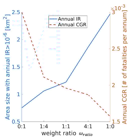
Figure 7.
Changes in annual IR and Annual CGR with risk weight ratios.
In summary, as the risk weight ratio increases, the paths detour more to low populated areas, and more flights have lower CGRfh. The annual CGR also reduces, but there are more areas that have high annual IRs. CGRfh is reduced because fewer people will beome fatally injured if paths detour over low populated areas, and the annual CGR is reduced for the same reason. However, because many flights occur over low-populated areas, people living in these areas are more likely to be injured by drones, making the annual IR in these areas high. Thus, there are more areas that have high annual IR. In addition, considering the thresholds for different TPR indicators, CGRfh is satisfied for all tested risk weight ratios, and annual CGR is only satisfied with 1:0; moreover, areas that have high annual IR always exist.
4.2. Experiment II: # of Packages per Person per Annum
This experiment evaluates how TPR changes as the volume of flight operations increases by increasing the # of packages per person per annum. Here, the risk weight ratio is set as 1:1.
Here, we increase the # of packages per person per annum from 0.1 to 10. The generated paths are shown in Figure A2 in Appendix A. The CGRfh for different flight volumes is shown in Figure A3 in Appendix A. The range of CGRfh for the flights does not change, and the flight frequency for each CGRfh also does not change. The annual IR for different flight volumes is shown in Figure A4 in Appendix A. Color (Annual IR) becomes brighter (higher) intuitively in the figure. To compare the differences in annual IR quantitatively, we plot annual IRs as a series of box plots, as shown in Figure 8a. The annual CGR for different flight volumes is shown in Figure 8b. Annual CGRs increase linearly with the # of flights.
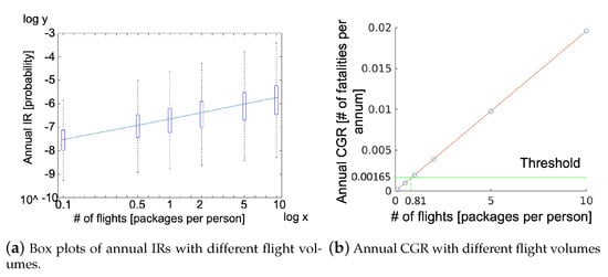
Figure 8.
Annual IR and annual CGR with different flight volumes.
4.3. Experiment III: Sensitivity Analysis on Parameters in Risk Assessment
This section simulates how parameters in risk assessment affect the estimated annual IR and annual CGR. A total of six parameters is included: the failure rate that reflects system stability, the mean drag coefficient , the drone’s surface area size , and wind velocity w that affects the ballistic descent process. Moreover, parameters a and b are in the RCC fatality model. Here, a and b do not have physical meaning, but they affect the estimation of calculated fatality probability.
The range of values for each parameter is shown in Table 4. In these experiments, is time-invariant. The range of is determined based on [46]. For areas varying from urban areas to city centers where the population density is larger than 3861 persons/km and for the drone’s weight varying from <0.5 kg to 25 kg, the maximum acceptable changes from [1.50 × 10 to 1.28 × 10. The drag coefficient varies for different shapes. For most shapes, is within range [47]. The surface area size of most small UAs is in the range of [0.1 m, 0.4 m] [46]. To conduct sensitivity analyses on wind, we retain the wind direction but proportionally change wind speeds. Let be the recorded wind speed in the data; then, we take as the wind speed for risk assessments, and the varies in . The RCC fatality model is a fitted model based on fatality data. The fatality probabilities are different if the object hits different body positions. The authors of [45] fit a and b for the probability of fatality from debris impacts for different body positions. a is in and b is in . Here, we take a and b from a larger range of and separately, which covers the fatality probability of a drone hitting a person.
Table 4.
Parameters in risk assessments and their values for sensitivity analyses.
4.3.1. Sensitivity Analysis for Failure Model
The failure model contains parameter failure rate . The annual IR for different is shown in Figure A5 in Appendix A. As reduces from 1.50 × 10 to 1.28 × 10, the maximum IR reduces from 4.20 × 10 to 3.60 × 10, and CGR reduces from 8.58 × 10 to 7.32 × 10. The box plots of the annual IR for different is shown in Figure 9a, and the annual CGR is shown in Figure 9b. Both annual IR and annual CGR have linear relationships with . As failure rate increases, the ground crash probability increases linearly; thus, the individual risk per flight will increase linearly. Based on Equations (1) and (3), the annual IR and annual CGR will also increase linearly, which corresponds to the obtained simulation results.
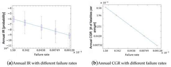
Figure 9.
Annual IR and Annual CGR with different failure rates.
4.3.2. Sensitivity Analysis for Descent Model
The descent model contains the following parameters: mean drag coefficient , surface area size of drones, and wind speed w. The annual IR for different is shown in Figure 10. As increases, the width of colored areas increases, meaning that drones can drop to places further away from the nominal paths; thus, areas affected by drone operations enlarge. The annual CGR for different is shown in Table 5. It increases from 1.74 × 10 fatalities per annum to 2.07 × 10 fatalities per annum as increases. This can be understood from the impact energy and impact position’s perspective.
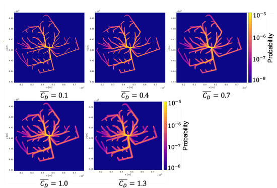
Figure 10.
Annual IRs with different mean drag coefficients .
Table 5.
Annual CGRs for different , , and w.
The case of the velocity and energy of a drone crashing to the ground for different is shown in Table 6. As increases, the vertical speed of the drone crashing to the ground reduces from 50.6 m/s to 21.7 m/s because of a larger drag force. Since vertical speeds account most for the total speed, the impact’s energy reduces significantly from 4719 Joule to 926 Joule. However, this impact energy is still very large, and it almost causes a fatality if it hits a person. At the same time, as increases, drones are more likely to fly away from the nominal path because of wind. Since the nominal paths are over low-populated areas, such deviation results in the impact location having a higher population. As a result, the annual IR becomes scattered because of the deviation of the impact location, the annual CGR increases because the population at the impact location is higher while the fatality probability for hitting a person almost does not reduce.
Table 6.
A case of velocity and energy when crashing to the ground for different .
In summary, as increases, the annual IR is more scattered over the considered area, and the annual CGR increases at the same time. The annual IR for different and w are shown in Figure A6 and Figure A7 in Appendix A. The width of the colored areas increases, similarly to . The annual CGRs for different and w are shown in Table 5. Either the increase in or w makes the annual CGR increase, similarly to .
4.3.3. Sensitivity Analysis for Fatality Model
The fatality model contains two parameters a and b. The annual IR for different a and b is shown in Figure A8 and Figure A9 in Appendix A. The annual CGR for different a and b are shown in Table A2 in Appendix A. We can see that both annual CGR and annual IR almost do not change for different a and b. The reason is that because the impact energy is too large, such as in Table 6 where the minimum impact energy is still 926 J. Whatever model is taken, hitting a person almost results in a fatality.
5. Discussion for Simulation Results
This section discusses the societal effect of using state-of-the-art risk-aware path planning when mitigating risks.
Based on the simulation results in Section 4, risk-aware path planning does not necessarily generate paths that meet the annual TPR criteria, as it depends on the risk weight ratio and flight volume. Because the trend of annual IRs and annual CGRs with the risk weight ratio is contradictory for current path planning, adjusting the risk weight ratio to reduce annual CGR/IR will definitely increase another. Trading off the risk weight ratio can make both annual IR and annual CGR acceptable in some cases but not in all cases. In addition, once the flight volume is larger than a certain threshold, the annual TPR criteria can not always be satisfied by UAS path planning alone, such as in the above-tested scenario in which the certain annual threshold is small. In this case, one possible way to reduce TPR is to reduce the system’s failure rate. In addition, when increasing the drag coefficient, the impact’s speed will reduce; thus, the impact energy will be reduced. However, drones may fly over more populated areas, as a result of which the annual CGR may even increase.
Based on the discussion, we can give the following meaningful insights:
- 1.
- For annual flights, current UAS path planning can reduce CGRfh and annual CGR but it may lead to more areas with a high annual IR. The trade-off on weight risk ratio in current UAS path planning should be carefully considered.
- 2.
- Annual IR and annual CGR increase linearly as the number of flights increases. Current UAS path planning fails to generate paths that satisfy safety risk criteria if the flight volume is larger than a certain threshold.
- 3.
- Both the annual IR and annual CGR reduce linearly as the system’s failure rate reduces.
- 4.
- Increasing the drag coefficient reduces the impact energy, but drones can fly away to highly populated areas.
6. Conclusions
This paper focuses on the safety risk posed by multiple unmanned aircraft flights to people on the ground in urban areas. Many UAS risk-aware path-planning methods in the literature have been developed to reduce the risk for a single flight, but it is unknown whether they are effective for reducing societal third-party risks. So this paper assesses the societal third-party risk of using state-of-the-art risk-aware path planning instead of shortest-paths via a simulation study.
Two third-party risk indicators that consider societal effects, annual individual risk and annual collective ground risk, are assessed in the work. Moreover, one commonly used indicator for a single flight, the collective ground risk per flight hour, is also involved in the comparison. Definitions of these indicators are introduced in Section 2.
The proposed method in Section 3 evaluates how the third-party risks change when risk weight ratio in path planning, flight volume, and risk assessment parameters change. The method is applied in a scenario of a UAS parcel delivery service for the city of Delft in the Netherlands. The simulation results and the discussions are in Section 4 and Section 5, respectively.
Future works will focus on developing path-planning methods that consider operation volumes for making acceptable-level collective ground and individual risks. In addition, we will explore methods and techniques for reducing impact risks during descents, such as using parachutes, and evaluate their effectiveness on reducing societal third-party risks.
Author Contributions
Conceptualization, L.L. and H.B.; methodology, X.H. and C.J.; software, X.H.; validation, X.H.; formal analysis, X.H. and C.J.; investigation, X.H.; resources, X.H. and C.J.; data curation, X.H.; writing—original draft preparation, X.H.; writing—review and editing, L.L. and H.B.; visualization, X.H.; supervision, L.L. and H.B.; project administration, L.L.; funding acquisition, L.L. All authors have read and agreed to the published version of the manuscript.
Funding
This research was funded by the Hong Kong Research Grants Council (General Research Fund, Project No. 11215119 and 11209717) and City University of Hong Kong Strategic Research Grant (Project No. 7005569).
Data Availability Statement
Not applicable.
Acknowledgments
The authors gratefully acknowledge the support of Hong Kong Research Grants Council and City University of Hong Kong Strategic Research Grant. The authors gratefully acknowledge Air Transport and Operations, Faculty of Aerospace Engineering, Delft University of Technology, for hosting the visit. In addition, we thank the editors and reviewers for contributing to the final form of this research.
Conflicts of Interest
The authors declare no conflict of interest.
Appendix A

Figure A1.
Histogram of CGRfh with different risk weight ratios.

Figure A2.
Generated paths for OD pairs in Experiment II.

Figure A3.
CGRfh with different flight volumes.

Figure A4.
Annual IR with different flight volumes.

Figure A5.
Annual IR with different failure rate .

Figure A6.
Annual IR with different surface area size .

Figure A7.
Annual IR with different wind speed w.

Figure A8.
Annual IR with different a in fatality model.

Figure A9.
Annual IR with different b in fatality model.
Table A1.
Summary of risk assessment model parameters.
Table A1.
Summary of risk assessment model parameters.
| Model in Risk Assessment | Parameter | Value |
|---|---|---|
| Failure model | failure rate (per hour) | 3.42 × 10 [46] |
| Descent model | drag coefficient | [43] |
| surface area (m) | ||
| wind speed w | from KNMI [48] | |
| Fatality model | mid-point value a(Joule) | 101.6 [45] |
| standard deviation b | 0.538 [45] | |
| Others | mass with parcel m [kg] | 3.7 [40] |
| cruise speed (m/s) | 12 [41] | |
| ascent speed (m/s) | 7.5 [41] | |
| descent speed (m/s) | 6 [41] | |
| horizontal position errors (m) | 3.68 [42] | |
| vertical position errors (m) | 7.65 [42] | |
| horizontal velocity errors (m/s) | 2.0 [43] | |
| vertical velocity errors (m/s) | 2.0 [43] |
Table A2.
Annual CGR with different a and b.
Table A2.
Annual CGR with different a and b.
| a | 53 | 103 | 153 | 203 | 253 |
| Annual CGR (# of fatalities per annum) | 1.96 × 10 | 1.96 × 10 | 1.95 × 10 | 1.94 × 10 | 1.93 × 10 |
| b | |||||
| Annual CGR (# of fatalities per annum) | 1.96 × 10 | 1.96 × 10 | 1.96 × 10 | 1.95 × 10 | 1.94 × 10 |
References
- ICAO. Unmanned Aircraft Systems (UAS); Circular 328-AN/190; International Civil Aviation Organization: Montreal, QC, Canada, 2011. [Google Scholar]
- Kersten, H.; Benedikt, K.; Robin, R. Advanced Air Mobility in 2030. 2021. Available online: https://www.mckinsey.com/industries/aerospace-and-defense/our-insights/advanced-air-mobility-in-2030 (accessed on 2 November 2022).
- MorganStanley. eVTOL/Urban Air Mobility TAM Update: A Slow Take-Off, But Sky’s the Limit. 2021. Available online: https://assets.verticalmag.com/wp-content/uploads/2021/05/Morgan-Stanley-URBAN_20210506_0000.pdf (accessed on 2 November 2022).
- Goerzen, C.; Kong, Z.; Mettler, B. A survey of motion planning algorithms from the perspective of autonomous UAV guidance. J. Intell. Robot. Syst. 2010, 57, 65–100. [Google Scholar] [CrossRef]
- Dijkstra, E.W. A note on two problems in connexion with graphs. Numer. Math. 1959, 1, 269–271. [Google Scholar] [CrossRef]
- Hart, P.E.; Nilsson, N.J.; Raphael, B. A Formal Basis for the Heuristic Determination of Minimum Cost Paths. IEEE Trans. Syst. Sci. Cybern. 1968, 4, 100–107. [Google Scholar] [CrossRef]
- Koenig, S.; Likhachev, M. Fast replanning for navigation in unknown terrain. IEEE Trans. Robot. 2005, 21, 354–363. [Google Scholar] [CrossRef]
- Daniel, K.; Nash, A.; Koenig, S.; Felner, A. Theta*: Any-angle path planning on grids. J. Artif. Intell. Res. 2010, 39, 533–579. [Google Scholar] [CrossRef]
- Kavraki, L.E.; Švestka, P.; Latombe, J.C.; Overmars, M.H. Probabilistic roadmaps for path planning in high-dimensional configuration spaces. IEEE Trans. Robot. Autom. 1996, 12, 566–580. [Google Scholar] [CrossRef]
- Lavalle, S.M. Rapidly-Exploring Random Trees: A New Tool for Path Planning; Technical Report; Iowa State University: Ames, IA, USA, 1998. [Google Scholar]
- Karaman, S.; Frazzoli, E. Sampling-based algorithms for optimal motion planning. Int. J. Robot. Res. 2011, 30, 846–894. [Google Scholar] [CrossRef]
- Primatesta, S.; Rizzo, A.; la Cour-Harbo, A. Ground risk map for unmanned aircraft in urban environments. J. Intell. Robot. Syst. 2020, 97, 489–509. [Google Scholar] [CrossRef]
- Guglieri, G.; Lombardi, A.; Ristorto, G. Operation oriented path planning strategies for rpas. Am. J. Sci. Technol. 2015, 2, 1–8. [Google Scholar]
- Primatesta, S.; Guglieri, G.; Rizzo, A. A risk-aware path planning strategy for UAVs in urban environments. J. Intell. Robot. Syst. 2019, 95, 629–643. [Google Scholar] [CrossRef]
- Primatesta, S.; Cuomo, L.S.; Guglieri, G.; Rizzo, A. An innovative algorithm to estimate risk optimum path for unmanned aerial vehicles in urban environments. Transp. Res. Procedia 2018, 35, 44–53. [Google Scholar] [CrossRef]
- Hu, X.; Pang, B.; Dai, F.; Low, K.H. Risk Assessment Model for UAV Cost-Effective Path Planning in Urban Environments. IEEE Access 2020, 8, 150162–150173. [Google Scholar] [CrossRef]
- Rudnick-Cohen, E.; Herrmann, J.W.; Azarm, S. Risk-based path planning optimization methods for unmanned aerial vehicles over inhabited areas. J. Comput. Inf. Sci. Eng. 2016, 16, 021004. [Google Scholar] [CrossRef]
- Primatesta, S.; Scanavino, M.; Guglieri, G.; Rizzo, A. A risk-based path planning strategy to compute optimum risk path for unmanned aircraft systems over populated areas. In Proceedings of the 2020 International Conference on Unmanned Aircraft Systems (ICUAS), Athens, Greece, 1–4 September 2020; pp. 641–650. [Google Scholar]
- Weibel, R.; Hansman, R.J. Safety considerations for operation of different classes of UAVs in the NAS. In Proceedings of the AIAA 3rd “Unmanned Unlimited” Technical Conference, Workshop and Exhibit, Chicago, IL, USA, 20–23 September 2004; p. 6421. [Google Scholar]
- Lum, C.W.; Waggonery, B. A risk based paradigm and model for unmanned aerial systems in the national airspace. In Proceedings of the AIAA Infotech at Aerospace Conference and Exhibit 2011, St. Louis, MO, USA, 29–31 March 2011. [Google Scholar] [CrossRef]
- Dalamagkidis, K.; Valavanis, K.P.; Piegl, L.A. On Integrating Unmanned Aircraft Systems into the National Airspace System; Springer: Dordrecht, The Netherlands, 2012; pp. 1–305. [Google Scholar] [CrossRef]
- Clothier, R.; Walker, R. Determination and evaluation of UAV safety objectives. In Proceedings of the 21st International Conference on Unmanned Air Vehicle Systems, University of Bristol, Bristol, UK, 3–5 April 2006; pp. 18–21. [Google Scholar]
- Bohnenblust, H. Risk-based decision making in the transportation sector. In Quantified Societal Risk and Policy Making; Springer: Berlin/Heidelberg, Germany, 1998; pp. 132–153. [Google Scholar]
- Ale, B.; Piers, M. The assessment and management of third party risk around a major airport. J. Hazard. Mater. 2000, 71, 1–16. [Google Scholar] [CrossRef]
- Smets, H. Frequency Distribution of the Consequences of Accidents Involving Hazardous Substances in OECD Countries. 1996. Available online: https://www.oecd.org/officialdocuments/publicdisplaydocumentpdf/?doclanguage=en&cote=ocde/gd(97)31 (accessed on 2 November 2022).
- Laheij, G.; Post, J.; Ale, B. Standard methods for land-use planning to determine the effects on societal risk. J. Hazard. Mater. 2000, 71, 269–282. [Google Scholar] [CrossRef]
- Bottelberghs, P. Risk analysis and safety policy developments in the Netherlands. J. Hazard. Mater. 2000, 71, 59–84. [Google Scholar] [CrossRef]
- Jonkman, S.; Van Gelder, P.; Vrijling, J. An overview of quantitative risk measures for loss of life and economic damage. J. Hazard. Mater. 2003, 99, 1–30. [Google Scholar] [CrossRef]
- Trbojevic, V. Risk criteria in EU. Risk 2005, 10, 1945–1952. [Google Scholar]
- Blom, H.A.P.; Jiang, C.; Grimme, W.B.A.; Mitici, M.; Cheung, Y.S. Third party risk modelling of Unmanned Aircraft System operations, with application to parcel delivery service. Reliab. Eng. Syst. Saf. 2021, 214, 107788. [Google Scholar] [CrossRef]
- Bertrand, S.; Raballand, N.; Viguier, F.; Muller, F. Ground risk assessment for long-range inspection missions of railways by UAVs. In Proceedings of the 2017 International Conference on Unmanned Aircraft Systems (ICUAS), Miami, FL, USA, 13–16 June 2017; pp. 1343–1351. [Google Scholar]
- Ancel, E.; Capristan, F.M.; Foster, J.V.; Condotta, R.C. Real-time risk assessment framework for unmanned aircraft system (UAS) traffic management (UTM). In Proceedings of the 17th Aiaa Aviation Technology Integration, and Operations Conference, Denver, CO, USA, 5–9 June 2017; p. 3273. [Google Scholar]
- la Cour-Harbo, A.; Schiøler, H. Probability of Low-Altitude Midair Collision Between General Aviation and Unmanned Aircraft. Risk Anal. 2019, 39, 2499–2513. [Google Scholar] [CrossRef]
- Dalamagkidis, K.; Valavanis, K.P.; Piegl, L.A. On Integrating Unmanned Aircraft Systems into the National Airspace System: Issues, Challenges, Operational Restrictions, Certification, and Recommendations; Springer: Berlin/Heidelberg, Germany, 2009. [Google Scholar]
- la Cour-Harbo, A. Quantifying risk of ground impact fatalities for small unmanned aircraft. J. Intell. Robot. Syst. 2019, 93, 367–384. [Google Scholar] [CrossRef]
- He, X.; He, F.; Li, L.; Zhang, L.; Xiao, G. A Route Network Planning Method for Urban Air Delivery. arXiv 2022, arXiv:2206.03085. [Google Scholar] [CrossRef]
- Benarbia, T.; Kyamakya, K. A literature review of drone-based package delivery logistics systems and their implementation feasibility. Sustainability 2021, 14, 360. [Google Scholar] [CrossRef]
- Waris, I.; Ali, R.; Nayyar, A.; Baz, M.; Liu, R.; Hameed, I. An Empirical Evaluation of Customers’ Adoption of Drone Food Delivery Services: An Extended Technology Acceptance Model. Sustainability 2022, 14, 2922. [Google Scholar] [CrossRef]
- Hill, C.; Garrow, L.A. A Market Segmentation Analysis for an eVTOL Air Taxi Shuttle. In Proceedings of the AIAA AVIATION 2021 FORUM, Online, 2–6 August 2021; p. 3183. [Google Scholar]
- Microdrones. md4-1000: Robust and Powerful—UAV /Drone Model from Microdrones. Available online: https://www.microdrones.com/en/drones/md4-1000/ (accessed on 2 November 2022).
- DJI. Inspire 2—Specs. Available online: https://www.dji.com/nl/inspire-2/specs (accessed on 2 November 2022).
- Grimes, J.G. Global Positioning System Standard Positioning Service Performance Standard; Tech. Rept; Department of Defense, Global Positioning System: Washington, DC, USA, 2008.
- la Cour-Harbo, A. Ground impact probability distribution for small unmanned aircraft in ballistic descent. In Proceedings of the 2020 International Conference on Unmanned Aircraft Systems (ICUAS), Athens, Greece, 1–4 September 2020; pp. 1442–1451. [Google Scholar]
- Range Commanders Council. Range Safety Criteria for Unmanned Air Vehicles, Rationale and Methodology Supplement; Supplement to Document 321-00; Range Commanders Council: Albuquerque, NM, USA, 2000. [Google Scholar]
- Range Commanders Council. Common Risk Criteria for National Test Ranges; Supplement to Standard 321-00; Range Commanders Council: Albuquerque, NM, USA, 2000. [Google Scholar]
- Melnyk, R.; Schrage, D.; Volovoi, V.; Jimenez, H. A third-party casualty risk model for unmanned aircraft system operations. Reliab. Eng. Syst. Saf. 2014, 124, 105–116. [Google Scholar] [CrossRef]
- Baker, W.E.; Cox, P.; Kulesz, J.; Strehlow, R.; Westine, P. Explosion Hazards and Evaluation; Elsevier: Amsterdam, The Netherlands, 2012. [Google Scholar]
- KNMI. Uurgegevens van het Weer in Nederland. Available online: https://projects.knmi.nl/klimatologie/uurgegevens/selectie.cgi (accessed on 2 November 2022).
Publisher’s Note: MDPI stays neutral with regard to jurisdictional claims in published maps and institutional affiliations. |
© 2022 by the authors. Licensee MDPI, Basel, Switzerland. This article is an open access article distributed under the terms and conditions of the Creative Commons Attribution (CC BY) license (https://creativecommons.org/licenses/by/4.0/).