Article

An Uncertainty Weighted Non-Cooperative Target Pose Estimation Algorithm, Based on Intersecting Vectors

1
School of Mechatronic Engineering and Automation, Shanghai University, Shanghai 200444, China
2
Marine Engineering College, Dalian Maritime University, Dalian 116026, China
*
Author to whom correspondence should be addressed.
Aerospace 2022, 9(11), 681; https://doi.org/10.3390/aerospace9110681
Submission received: 19 September 2022 / Revised: 27 October 2022 / Accepted: 1 November 2022 / Published: 3 November 2022
(This article belongs to the Section Astronautics & Space Science)

Abstract

:
Aiming at the relative pose estimation of non-cooperative targets in space traffic management tasks, a two-step pose estimation method, based on spatially intersecting straight lines, is proposed, which mainly includes three aspects: (1) Use binocular vision to reconstruct the straight space line, and based on the direction vector of the straight line and the intersection of the straight line, solve the pose of the measured target in the measurement coordinate system, and obtain the initial value of the pose estimation. (2) Analyze the uncertainty of the spatial straight-line imaging, construct the uncertainty description matrix of the line, and filter the line features, accordingly. (3) Analyze the problems existing in the current linear distance measurement, construct the spatial linear back-projection error in the parametric coordinate space, and use the linear imaging uncertainty to weigh the projection error term to establish the optimization objective function of the pose estimation. Finally, the nonlinear optimization algorithm is used to iteratively solve the above optimization problem, to obtain high-precision pose estimation results. The experimental results show that the two-step pose estimation algorithm, proposed in this paper, can effectively achieve a high-precision and robust pose estimation for non-cooperative spatial targets. When the measurement distance is 10 m, the position accuracy can reach 10 mm, and the attitude measurement accuracy can reach 1°, which meets the pose estimation accuracy requirements of space traffic management.

1. Introduction

The relative pose estimation is one of the basic technologies of space on-orbit operations and traffic management tasks [1,2,3]. For the estimation of the relative pose between spacecrafts, the ground telemetry method cannot obtain the high-precision 6-DoF (six-degree-of-freedom) parameters [4]. In recent years, pose estimation methods, based on LiDAR (light detection and ranging) and vision, have been favored by researchers [5]. LiDAR is not restricted by light conditions. However, LiDAR is an active sensor, the data it collects is sparse, and the power consumption and quality are large. Therefore, it is difficult to obtain high-precision measurement results in tasks, such as space traffic management. Compared with the LiDAR-based method, the vision-based method has the advantages of a low price, low power consumption, lightweight, and full-field measurements. Therefore, the vision-based method is widely used in aerospace missions [6].
For the relative pose estimation of non-cooperative spacecrafts, based on vision, there are currently mainly model-based methods, point-based methods, line-based methods, and deep learning-based methods [7]. The method, based on the model, is referred to the use of the camera images and the feature information of the observed building geometry model (such as shape, and size), and then with the known model is combined with the corresponding information for the reference estimation algorithm for the pose parameters, but this kind of method needs to know the geometry prior to the information of the target [8,9]. Therefore, its application scope is greatly limited. Based on the deep learning method, the use of the offline training network model for the non-cooperation target pose estimation, and then the images captured by the camera in real-time are processed online to achieve the relative pose estimation [10,11,12]. This method has a good robustness and is not sensitive to light, but it needs a lot of offline data to train the estimation network. However, this process of the pose estimation of non-cooperative targets is not easy. A method, based on the point feature, refers to extracting the feature points of the non-cooperative target, and then, based on the known geometry information, or by using stereo vision ways to realize the feature points of the 3D (three dimensional) reconstruction, adopt the corresponding pose estimation algorithm for the pose estimation [13,14,15]. The algorithm is simple to implement, therefore the pose estimation, based on the cooperative target, is widely used. However, this method is easy to be affected by illumination conditions, and the algorithm’s robustness is poor. The method, based on the online feature, uses the information of the line and the conic section in the collected image, combined with the stereo vision to realize the estimation of the pose parameters. Compared with the feature point method, this method has a stronger robustness, so it has received extensive attention in recent years. Pose estimation methods, based on linear features, can be divided into a linear method and an iterative method. The linear solving algorithm is to directly use the known 3D model features or obtain a 3D model through stereo vision, and then solve the PnL (Perspective-n-Line) problems, such as the PnP (Perspective-n-Point) [16,17,18]. The iterative method usually uses the linear method to obtain the initial value and then uses the iterative algorithm to minimize the objective function to obtain the optimal pose estimation results [19,20]. The pose estimation method, based on the conic reconstruction, mainly uses the spatial analytic geometry theory and the perspective projection imaging model to solve the characteristic parameters of the spatial conic model in the closed form and obtain the pose estimation results [21]. In addition, the linear-based motion estimation algorithms are often used in tasks, such as in the robot estimation and aircraft ground simulation tests [22,23]. The main contributions of our work are as follows:
(1)
We propose a two-step relative pose estimation algorithm, based on the uncertainty analysis of the line extraction. The method fully considers the uncertainty of the straight-line extraction to weigh the error term of the objective function, and is more robust in a space environment than the feature-point-based method.
(2)
A novel distance error model for the reprojection of a line, in which the mean value of the distance sum from the two ends of the original direct comparison line segment to the line error, is transformed into the sum of the distance between the two points in the parameter space, which is more reasonable, in theory.
(3)
The proposed approach was verified on a ground test simulation environment and has been extensively evaluated in experimental and simulation analyses.
The rest of the paper is organized as follows: In Section 2, a new pose estimation method for non-cooperative targets, based on the line features, is presented, that extracts the intersection vectors and the intersection of the straight line from the target images. Then, the uncertainty of the straight-line extraction and the back-projection error model are analyzed, and the uncertainty model and straight-line error model are established in Section 3. Section 4 comments on the experimental results and Section 5 concludes the paper.

2. Principle of the Non-Cooperative Target Relative to the Pose Estimate

2.1. Problem Description of the Relative Pose Estimation

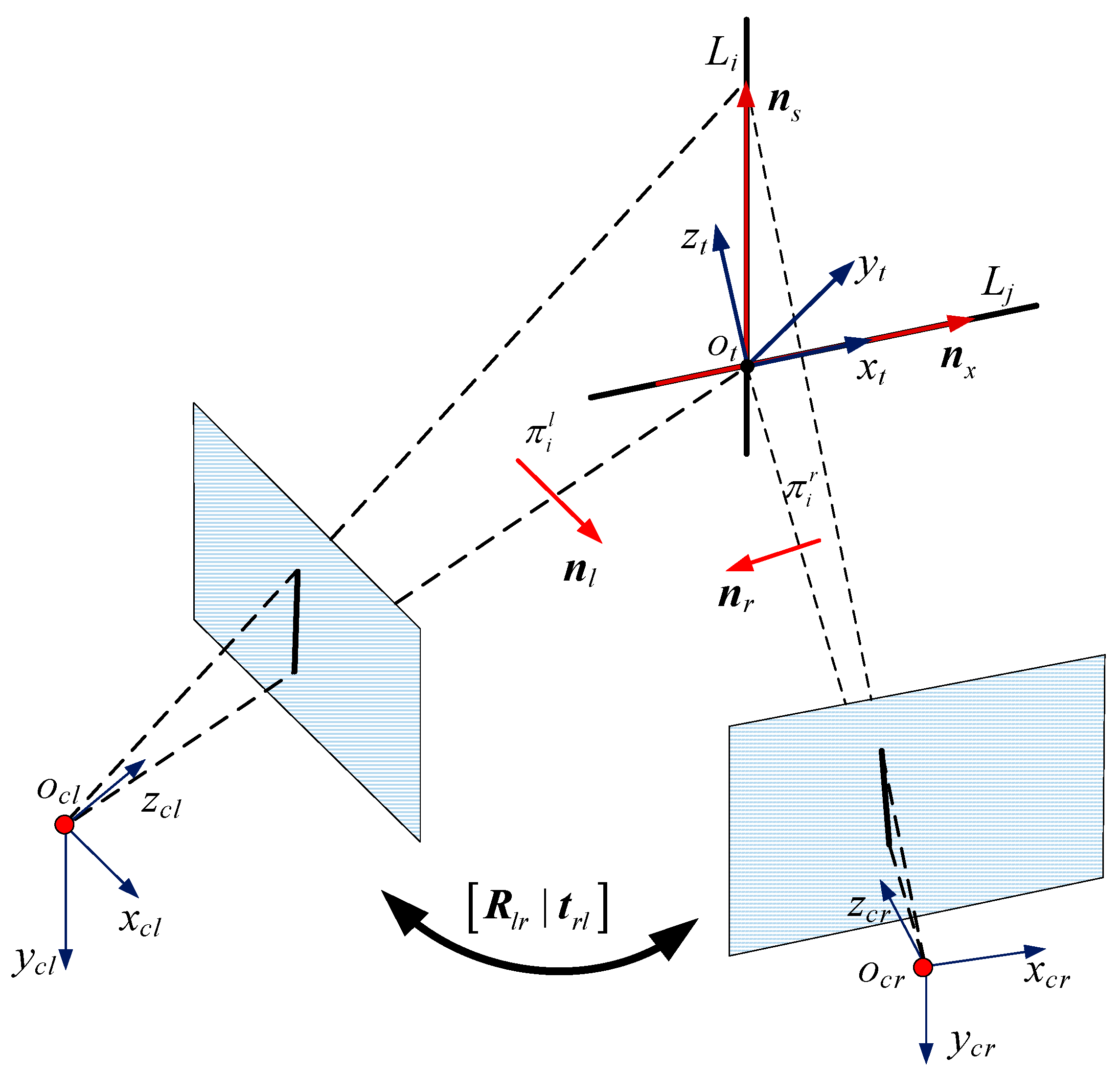
As shown in Figure 1, let the coordinate system of the measured target be O t x y z , The coordinate system of the binocular vision measurement unit is O b x y z . In this paper, it is assumed that it coincides with the left camera, L j represents the line feature on the target, j = 1 , , N f , N f is the number of lines, l i j l and l i j r represent the imaging of the straight line L i on the left and right cameras, and the left and right camera measurements are independent of each other, i represents the moment when the camera collects data. The internal and external calibration parameters of the binocular stereo vision measurement unit are [ A l , A r ] and [ R l r , T r l ] , respectively, and the calibration has been completed. Then, the relative pose estimation problem, based on the straight-line features, can be described as the following maximum a posteriori probability estimation problem:
How to estimate the rigid body transformation relationship x i and the spatial straight line L j between the coordinate system of the measured object and the coordinate system of the binocular measurement unit, according to the linear imaging l i l and l i r of the spatial straight line L j on the measured object in the left and right cameras:
X ¯ = arg max P ( x 1 : i | z 1 : i ) = arg max i = 1 N P ( L j , R b t i , T t b i | L j , R b t i 1 , T t b i 1 ) P ( l i j l , l i j r | L j , R b t i 1 , T t b i 1 ) ,
where x i represents the relative pose [ R b t i , T t b i ] and the spatial line L j of the target at different times, z i represents the spatial line feature and its imaging l i l and l i r in the camera, X ¯ represents the maximum posterior probability estimate of the relative pose.

2.2. Relative Pose Estimation between Spacecrafts

In order to solve the above-mentioned relative pose estimation problem, this paper proposes a relative pose estimation algorithm, which mainly includes two parts: (1) Solve the initial value of the relative pose estimation; (2) Iterative optimization of the relative pose estimation. The above two parts will be described in detail below.

2.2.1. Initial Value Solution of the Relative Pose Estimation, based on the Intersection Vector

Theorem 1.
If it is known that there are n 2 intersecting lines L i in the 3D space and their imaging l i l and l i r in the left and right views, and the internal and external parameters [ A l , A r , R l r , t r l ] of the binocular stereo vision have been calibrated, then the transformation matrix C t c = [ R t c | t c t ] between the visual measurement unit coordinate frame, relative to the target coordinate frame can be solved [23].
Proof of Theorem 1.
As shown in Figure 2, let the left camera coordinate system be the visual measurement unit coordinate system, if the spatial line set N of the target has been solved, then a line L i whose direction vector n x c is arbitrarily selected as the x-axis of the target coordinate frame, and then take any non-parallel line L j , whose direction vector is n s c , and take a cross product with n x c to obtain the y-axis direction vector of the target coordinate frame, as follows:
n y c = n x c × n s c ,
The z-axis direction vector of the target coordinate frame is obtained by the cross-product of the vectors:
n z c = n x c × n y c ,
Therefore, we can construct a new matrix:
D c = ( n x c , n y c , n z c ) , D t = ( n x t , n y t , n z t ) = I ,
where D c is the direction vector of the linear features in the camera coordinate system, D t is constructed as the direction vector of the coordinate axis of the camera coordinate system represented in the target coordinate system, and according to the construction principle of the target coordinate system, it is set as the identity matrix I . If it is assumed that R t c represents the rotation transformation relationship between the measurement unit coordinate system and the target coordinate system, then according to the definition of the transition relationship between the coordinate systems, we can write:
R t c = D t D c 1 ,
For the solution of the displacement vector t c t 0 , it can be obtained by the coordinate O t and O c of the straight line intersection in the target coordinate frame and the left camera coordinate frame (it is set to the measurement coordinate system), respectively:
t c t 0 = O t R t c O c ,
If the straight-line intersection in the target coordinate frame is taken as the origin of the target coordinate system, the above equation can be expressed as:
t c t 0 = R t c O c ,

2.2.2. Nonlinear Optimization of the Pose Estimation

The initial relative pose relationship between the ontology and the target was obtained by solving the problem in the previous section. Ideally, if you were to project the direction vector of the line from the target coordinate system back to the camera coordinate system, they would be equal, but because of the error, they would not be equal. Therefore, for the attitude estimation, Equation (8) is adopted in this paper for a nonlinear optimization solution:
E ( R l t ) = arg min R l t i = 1 M j ( l , r ) n i j R j t n i L Σ d 2 , s . t . R r l R l t = R r t ,
where R r l represents the binocular vision external rotation parameter, R j t represents the rotation transformation matrix between the camera coordinate system and the target coordinate system, and n i j represents the representation of the spatial straight line direction vector in the left and right camera coordinate system, n i L represents the direction vector of a 3D straight line in the target frame, Σ d for the orientation uncertainty.
For the displacement t l t 0 , firstly, the rotation transformation matrix R t l is obtained by the optimization solution Equation (8), and the initial value t l t 0 is obtained through the initial value solution method mentioned above. Then, the spatial straight lines are back-projected into the imaging plane, and the bundle adjustment algorithm is used to solve Equation (9) to obtain the final most pose estimation:
E ( R l t , t t l ) = arg min R l t , t t l i = 1 M j ( l , r ) ( K j 1 [ R l t j | t t l 0 j ] L i ) n i j Σ l 2 ,
wherein M represents the number of straight lines in the 3D space, L i represents a spatial line on a non-cooperative target, n i j represents the direction vector of the projected line of the 3D space straight line in the left and right cameras, K j represents the internal parameter matrix of the left and right cameras, Σ l represents the linear position uncertainty. The LM (Levenberg–Marquardt) optimization algorithm is used to solve the above two nonlinear optimization problems.

3. Line Features Reconstruction and the Uncertainty Analysis

3.1. Solving the 3D Space Straight Line and Its Intersection

According to the pose estimation algorithm proposed above, to realize the pose estimation of the non-cooperative target, the 3D space straight line equation needs to be solved, and the weighted uncertainty of the nonlinear optimization objective function of the pose estimation is determined. Therefore, this section first uses binocular vision to reconstruct the 3D space straight line, and then analyzes the uncertainty of the direction and position of the line imaging, and constructs its uncertainty description matrix.
As shown in Figure 2, it is assumed that the intrinsic parameters K i of the two cameras and the external parameters [ R r l , t r l ] between the two cameras have been calibrated. The images of a 3D space line in two views can be expressed as:
{ l l : a 1 u + b 1 v + c 1 = 0 l r : a 2 u + b 2 v + c 2 = 0 ,
The two analytic planes π i l and π i r passing through the spatial straight line can be expressed as:
{ π i l : A 1 x + B 1 y + C 1 z + D 1 = 0 π i r : A 2 x + B 2 y + C 2 z + D 2 = 0 ,
If the left camera coordinate frame is assumed to be the reference coordinate frame, then in the reference coordinate frame, a 3D space straight line can be expressed as:
{ u j = m 11 j x + m 12 j y + m 13 j z + m 14 j m 13 j x + m 23 j y + m 33 j z + m 34 j v j = m 21 j x + m 22 j y + m 23 j z + m 14 j m 13 j x + m 23 j y + m 33 j z + m 34 j ,
where j ( l , r ) , the projection matrix can be expressed as:
P j = ( m 11 m 12 m 13 m 14 m 21 m 22 m 23 m 24 m 31 m 32 m 33 m 34 ) ,
When j = r , P r = C l r M r = [ R l r , t l r ] M r . According to Equations (10)–(13), we can obtain:
{ A i = a i m 11 + b i m 31 m 21 B i = a i m 12 + b i m 32 m 22 C i = a i m 13 + b i m 34 m 23 D i = a i m 14 + b i m 34 m 24 ,
wherein ( a i , b i ) represents the coordinates of the points on the straight-line image. The direction vector of a straight line in the 3D space can be obtained by directly solving the following equations:
v = n l i × n r i = ( | B 1 C 1 B 2 C 2 | , | C 1 A 1 C 2 A 2 | , | A 1 B 1 A 2 B 2 | ) ,
Similarly, the solution can be obtained: [ v 1 , , v N ] . The intersection of the straight lines can be obtained by solving the above-mentioned 3D space straight lines (the straight lines of the different planes are the midpoints of the mid-perpendicular lines). For a detailed solution, please refer to [24].

3.2. Uncertainty Analysis of the Straight Line Extraction

As shown in Figure 3, the uncertainty of the feature extraction of a straight line can be described as the angle uncertainty Δ θ and radius uncertainty Δ ρ of the feature extraction of a straight line.

3.2.1. Uncertainty Modeling of the Straight Line

If the size of the uncertainty region in the parameter space is assumed to be: θ ( θ 0 Δ θ 1 , θ 0 + Δ θ 2 ) , then according to the cosine law, we know that the uncertainty Δ θ can be expressed as:
Δ θ = a r c cos l 1 l 2 | l 1 | | l 2 | ,
where l 1 = ( 1 , k 1 ) , l 2 = ( 1 , k 2 ) , k 1 and k 2 can be obtained by solving the inner tangent of the two ellipses, and the following equation can be obtained after sorting:
{ ( B 1 b + 2 C 1 k b + D 1 + E 1 k ) 2 4 ( A 1 + B 1 k + C 1 k 2 ) ( C 1 b 2 + E 1 b + F 1 ) = 0 ( B 2 b + 2 C 2 k b + D 2 + E 2 k ) 2 4 ( A 2 + B 2 k + C 2 k 2 ) ( C 2 b 2 + E 2 b + F 2 ) = 0 ,
In this formula, A i , B i , C i , D i , E i and F i are, respectively, the coefficients of the general equation of the ellipse with the positioning uncertainty of the two feature points on the line, which can be obtained from the positioning uncertainty of the points on the straight line as ellipse Λ e [25]. Therefore, the direction uncertainty d of the straight line can be expressed as:
d = [ cos Δ θ 0 0 0 sin Δ θ 0 0 0 1 ] ,
The position uncertainty of the straight line can define as ρ ( ρ min , ρ max ) , wherein Δ ρ = ρ max ρ min , then, according to the distance formula from the point to the line, we can get the position uncertainty of the straight line as:
Δ ρ = | b 1 b 2 | k 2 + 1 ,
wherein b 1 and b 2 can be obtained by solving the outer tangents of the two ellipses in Equation (17).
Therefore, the uncertainty model Σ l of the linear projection in the 3D space can be modeled as a combination of the orientation uncertainty and the position uncertainty:
Σ l = [ cos Δ θ 0 0 0 sin Δ θ 0 0 0 Δ ρ ] ,

3.2.2. Linear Filtering based on the Uncertainty Size

Assuming that the uncertainty covariance matrix of the 3D reconstruction of a spatial straight line is Λ L . The imaging of a 3D space straight line in each camera can be defined as l = ( l l T , l r T ) , and because they are independent of each other, the covariance matrix of the spatial line can be represented as:
Λ l = d i a g ( Λ l l , Λ l r ) ,
wherein Λ l j = d i a g ( cos θ j , sin θ j ) , j ( l , r ) . Moreover, according to Equations (11) and (12), it can be known that the 3D space straight line L = f ( l ) . Therefore, the covariance matrix of a straight line solution in the 3D space can be expressed as:
Λ L = J Λ l J T = f ( l ) l Λ l f ( l ) T l ,
wherein f ( l ) / l = [ f ( l ) / l l , f ( l ) / l r ] , f ( l ) / l i = [ f ( l ) / u i , f ( l ) / v i ] , i = l , r .
According to Equation (22), the uncertainty covariance matrix Λ L of the features of each straight line is calculated, and then the determinant size of the uncertainty covariance matrix is solved to exclude the feature straight lines with large uncertainties, so as to determine the lines participating in pose estimation and to improve the accuracy of the non-cooperative target pose estimation, based on the line.

3.3. Line Reprojection Error Analysis

The current reprojection error of the line is generally defined as the average distance between the two endpoints of the line segment and the line. As shown in Figure 4, this definition has the following problems:
(1)
When the detection line segment and the reprojection line are in the situation, as shown in (a) and (b), the error means the two lines are completely inconsistent with the length being equal.
(2)
When the detection line segment and the directional projection line are in the situation, as shown in (c) and (d), its position on the line directly affects the error when the direction vector of the line remains unchanged.
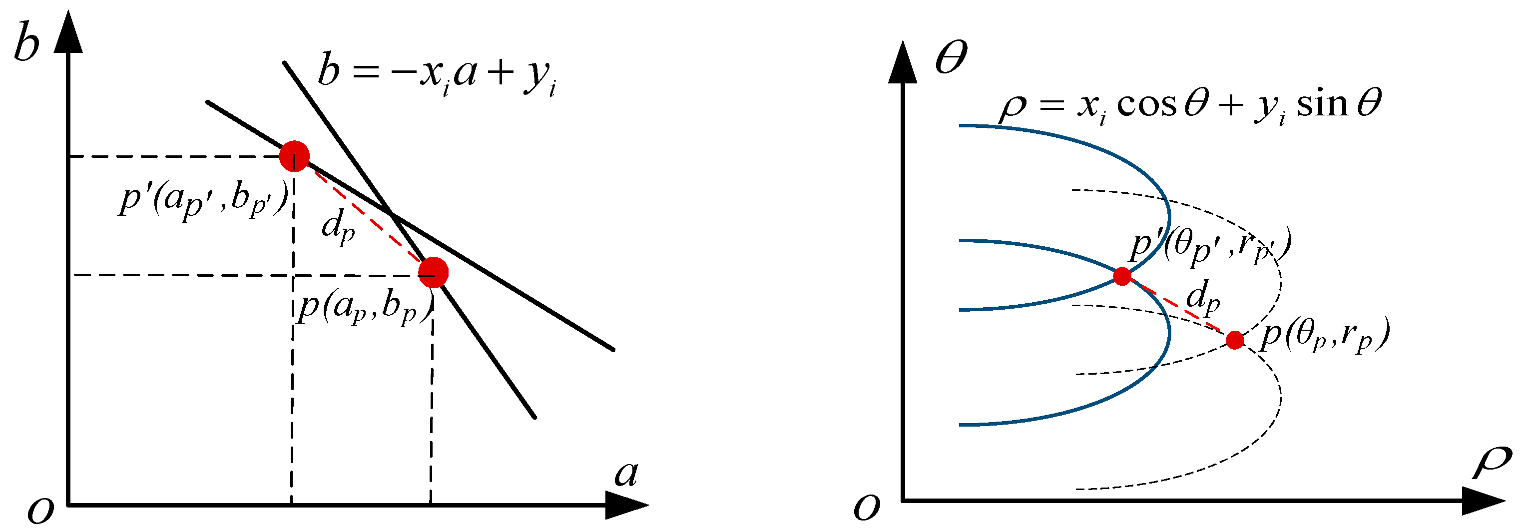
Intuitively, the difference between the two lines can be more accurately described by directly solving the “distance” between them. To solve the above problems, this paper transforms a straight line into a parametric space and defines the reprojection error of the straight line by solving the distance between the two points in the parametric space Cartesian coordinate system.
As shown in Figure 5, the line is in the parametric space Cartesian coordinate system:
b = x a   +   y ,
Using Cartesian coordinates to represent a line, when the line is a vertical line or nearly vertical line, the slope of the line is infinite or nearly infinite, and thus cannot be represented in the parameter space a-b. To solve this problem, we can use the statement in polar coordinates:
ρ = x cos θ + y sin θ   , ρ [ π / 2 , π / 2 ] ,
Therefore, according to the property that distance is independent of the coordinate system, the distance e p between the straight lines can be defined as:
e p = p p = ( θ p θ p ) 2 + ( ρ p ρ p ) 2 ,
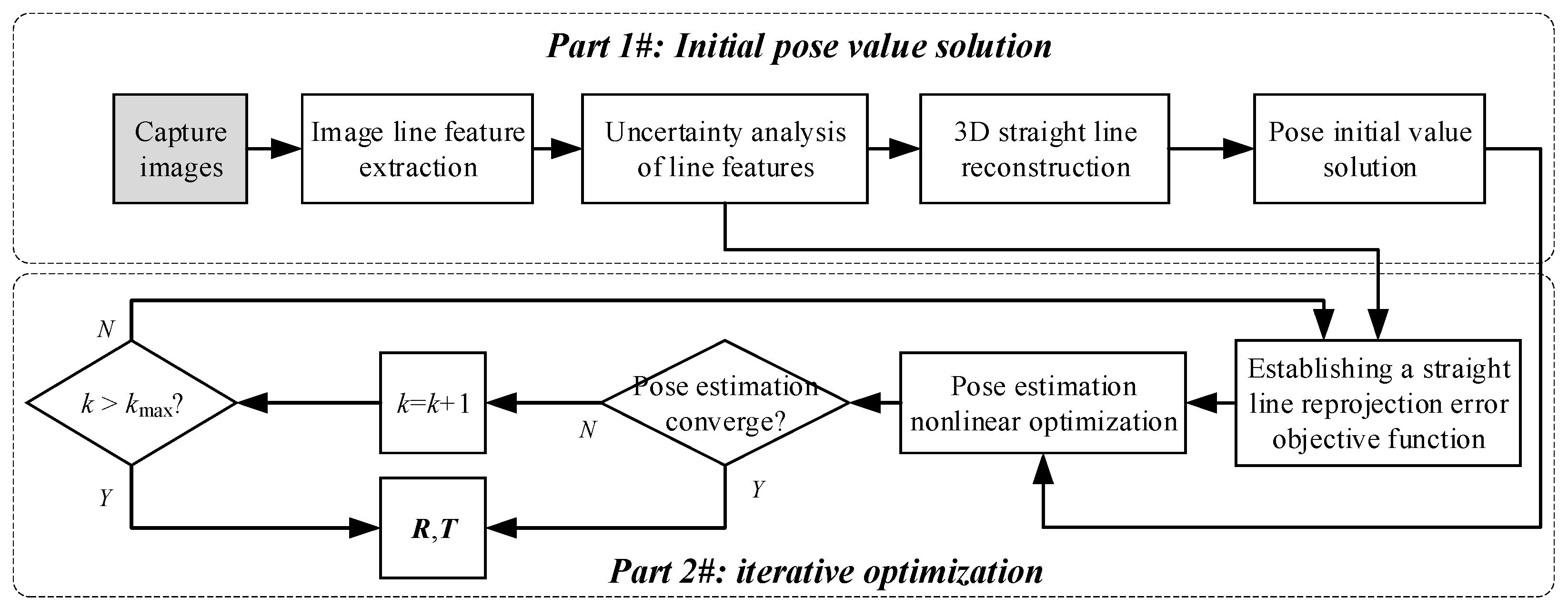
Once the uncertainty model of the straight line and the direction projection error model of the straight line is obtained, they can be brought into the nonlinear optimization objective function and solved iteratively by the nonlinear optimization algorithm, to obtain an accurate non-cooperative objective pose estimation. The algorithm flow of the non-cooperative target pose estimation, considering the straight line uncertainty, can be represented, as shown in Figure 6.

4. Experiments and Analysis

To verify the feasibility, the measurement accuracy, and the measurement robustness of the proposed non-cooperative pose estimation algorithm, a simulation analysis and test experiments were carried out, respectively, in this paper.

4.1. Simulation and Analysis

MATLAB simulation software is used to generate the feature point data on the line by the numerical simulation, and then the binocular vision algorithm is used to process the data offline to verify the performance of the different pose estimation algorithms. The simulation model of the target movement in the experiment is shown in Table 1.
In this section, a mathematical simulation model is established, according to the measurement requirements and the characteristics of the measurement target, and the Monte Carlo method is used for the simulation. The specific process of the numerical simulation is as follows: the 3D motion of four intersecting edge lines on the rigid body in the 3D space is simulated (its size is: 500 mm × 500 mm), the fixed noise was added to the intersecting points, between the lines, and the uncertainty of the point location in the stereo vision 3D positioning system was simulated by the Gaussian white noise with the mean value of 0 and the variance of 20 mm. For occlusion, several frames of the 3D point coordinate data were eliminated in a short time, in order to simulate. The target moves in the same direction from the position 12,000 mm to 2000 mm. The outer space non-cooperative target is in the slow spin instability state, and the slow spin motion parameters of the target are as follows: the spin angular velocity range is 1~10°/s, the maximum nutation angle: 10°. Finally, the pose estimation algorithm, based on the line features proposed in this paper is solved and compared with the direct linear method [20], the feature point method [12], and the odometer method [15].

4.1.1. Analysis of the Relationship between the Measurement Accuracy and the Measurement Frequency

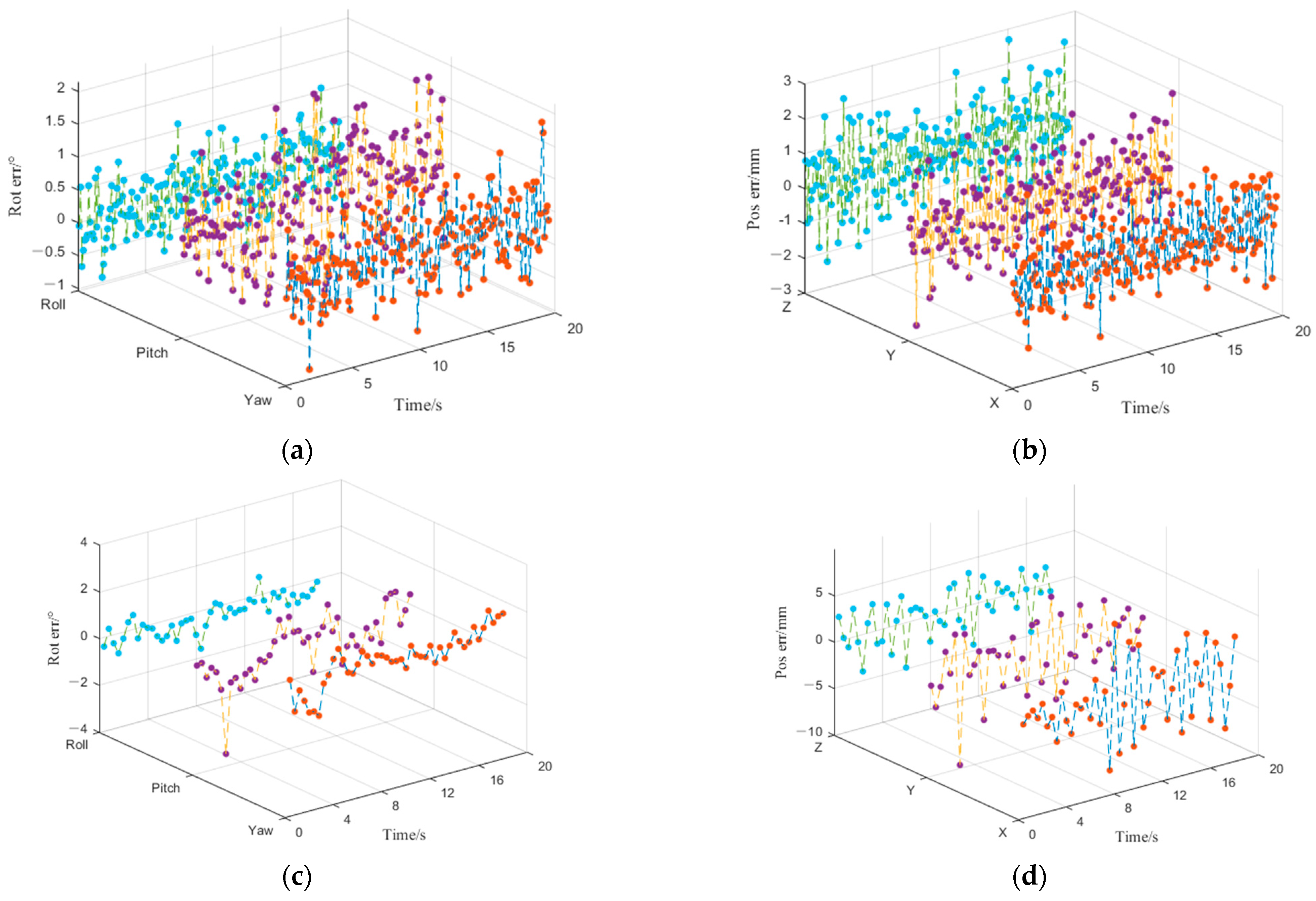
According to the actual research, the image acquisition frequency of general spaceborne high-resolution cameras does not exceed 10 Hz. To verify the relationship between the pose estimation algorithm and the sampling frequency of the measured data, this paper adopts the method of simulation analysis to simulate the measurement errors of the pose, when the data collection frequency is 10 Hz and 2.5 Hz, respectively, and make statistics. The results are shown in Figure 7.
Figure 7 shows the following results:
(1)
When the simulation data acquisition frequency is 10 Hz, the pose measurement results are shown in Figure 7a,b, the maximum measurement error of the attitude angle is less than 1° (3δ) and that of the position measurement is less than 2 mm (3δ), and the simulation results meet the pose measurement requirements.
(2)
When the data acquisition frequency is 2.5 Hz, the position and pose calculation results of the numerical simulation are shown in Figure 7c,d, the attitude measuring results had divergent trends in the shade, but the measurement error is bigger, this is due to the non-cooperative targets in space for the non-linear movement, and the amount of data collected is less, resulting in fewer constraints involved in the optimization using the linear model.
(3)
For the position measurement, it can be seen from Figure 7b,d that the position measurement is basically consistent with the theoretical setting value, and the position measurement results. By comparing the position measurement and attitude measurement results, the attitude measurement results are more sensitive to the 3D positioning accuracy, and the attitude measurement accuracy decreases significantly, compared with that when the sampling frequency is 10 Hz. This is mainly because the estimation hysteresis error, caused by the corresponding optimization algorithm, increases significantly with the decrease of the measurement data.

4.1.2. Algorithm Measurement Error Statistics and Analysis

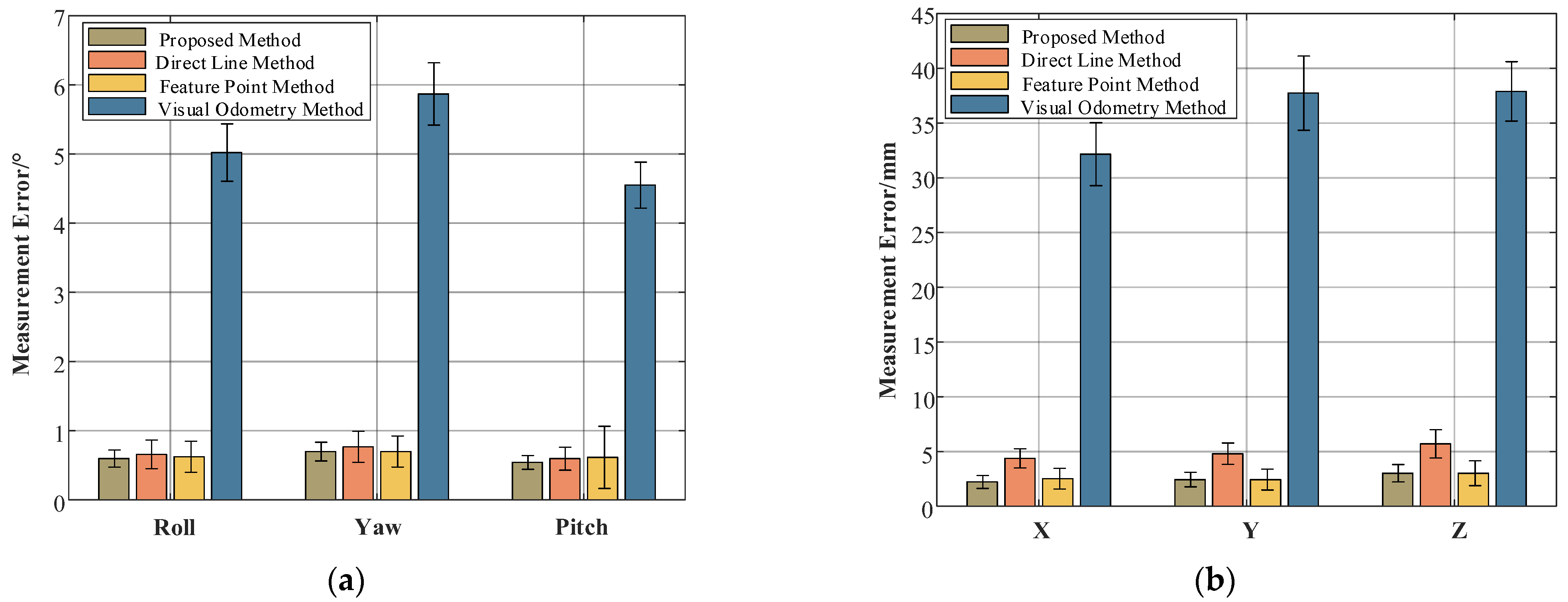
To verify the advantages of the algorithm proposed in this paper, compared with the direct linear method [20], the feature point method [12], and the visual odometry method [15], the mean value of the absolute error was counted. Firstly, the parameters of the simulation analysis were set, according to Table 1, and each method was simulated 100 times to obtain the mean value and variance. The results are shown in Figure 8.
Figure 8 shows the following results:
(1)
By comparing the measurement results of the four methods, the accuracy of the pose estimation algorithm of the visual odometry method is the worst, reaching the maximum attitude angle of 5.8° and the maximum position error of 37 mm. This is mainly because the visual odometer method has a cumulative error, so its error will become larger and larger as time goes by.
(2)
According to the attitude error of the measurement result, the measuring accuracy of the proposed algorithm, and based on the measuring accuracy of the feature point is quite up to 0.6°, the position is 2.2 mm, but this article proposed a smaller algorithm of the attitude angle variance, this is mainly because the participation attitude angle calculating the straight linear feature uses the linear reconstruction uncertainty size selection.
(3)
In the measurement results of the attitude angle, the errors of the pitch and yaw angles are large, and the z-axis errors of the position error are large, which is mainly caused by the great uncertainty of the vision measurement in the z-axis direction.

4.1.3. Comparison Experiment of the Algorithm Robustness

To verify the influence of the image measurement noise on the relative pose estimation algorithm of the non-cooperative targets, this paper uses the method of simulation analysis for the simulation verification. We use R t r u e and t t r u e to express the true value, meanwhile, R e s t and t e s t to express the value of the pose estimation. The r o t _ e r r ( % ) and p o s _ e r r ( % ) are described as:
{ p o s _ e r r ( % ) = t t r u e t e s t / t t r u e r o t _ e r r ( % ) = R t r u e R e s t / R t r u e ,
For the experimental results to be more statistically significant, we take the average of 100 times the experimental result under each parameter condition in this section.
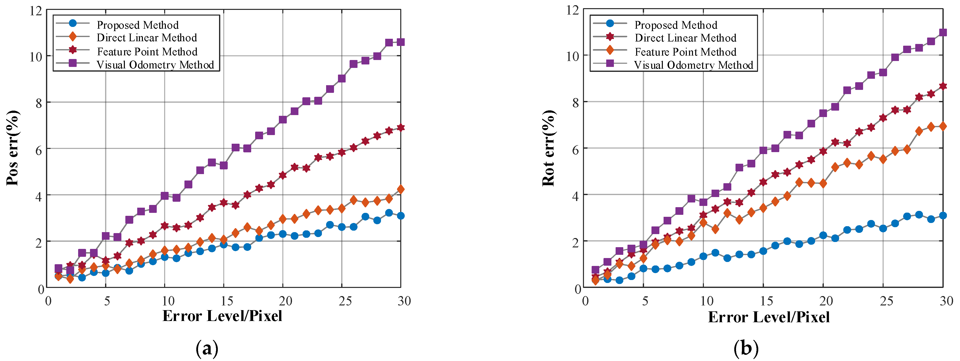
To evaluate the influence of the pose estimation results, under the noise of different levels, we set the number of feature points on the line as 20 for the feature points method and visual odometry method with the error mean value of 0, the variance σ 1 is varied from 1 to 30 pixels, and set the feature line number to eight for the direct linear method and the proposed method, and eight lines are constructed by using the above feature points directly.
Figure 9 shows the following results:
(1)
The measurement errors of the attitude and position points increase with the increase of the feature extraction errors, and the proposed calibration algorithm has the highest accuracy, compared with other algorithms participating in the comparison.
(2)
The algorithm proposed has a smaller error growth slope, compared with other algorithms, therefore this method has stronger robustness compared with other methods.
(3)
The position accuracy of the proposed algorithm is equivalent to that of the feature point method, mainly because it is equivalent, in theory, when the error level is the same. However, the algorithm proposed in this paper filters the straight lines involved in the pose estimation, so the positioning accuracy is slightly higher.

4.2. Actual Experiment and Analysis

To verify the pose estimation algorithm of the outer space non-cooperative target proposed in this paper, a set of binocular vision pose estimation systems is established. The system mainly includes two cameras with a resolution of 2048 × 2048 pixels and a pixel size of 0.0055 mm. A PC with a memory of 8 GB and a main frequency of 3.7 Hz; Two Zoom lens parameters are AF ZOOM-Nikon 24–85 mm/1:2.8-4D; A spacecraft with a natural size of 1000 mm × 900 mm and its motion simulator. The sampling frequency of the camera is 10 Hz; The algorithm is run in Matlab2017b.

4.2.1. Static Pose Estimation Experiment

Firstly, the binocular vision measurement system is calibrated. In this paper, the calibration algorithm, based on a planar target is adopted [26], and the calibration results are shown in Table 2.
Then, the feature point algorithm, the visual odometry algorithm, the direct linear algorithm, and the proposed algorithm are used to estimate the motion of the simulated spacecraft. The measurement results are shown in Table 3. The reference coordinate system of the pose parameters is the coordinate system of the simulated pose setting device, and the transformation relationship between it and the binocular vision measurement system is determined by using third-party calibration equipment (such as total station).
As shown in Table 3, except that the average error is close to the feature point-based method, both the average error and the maximum error of the algorithm proposed in this paper are more accurate than other algorithms, which indicates that the algorithm proposed in this paper has a better stability and accuracy.
Moreover, since the distance between the adjacent frames is far in the static experiment, the odometer-based algorithm cannot obtain enough matching feature points to solve the pose in most moments, due to the large illumination variation of the target surface coating layer.

4.2.2. Dynamic Pose Estimation Experiment

To verify the dynamic test performance of the algorithm proposed in this paper, the linear motion unit is used, the relative attitude of the target remains unchanged, the target moves in a uniform phase from 12 m to 2 m, and the binocular camera is used to capture the target image, as shown in Figure 10.
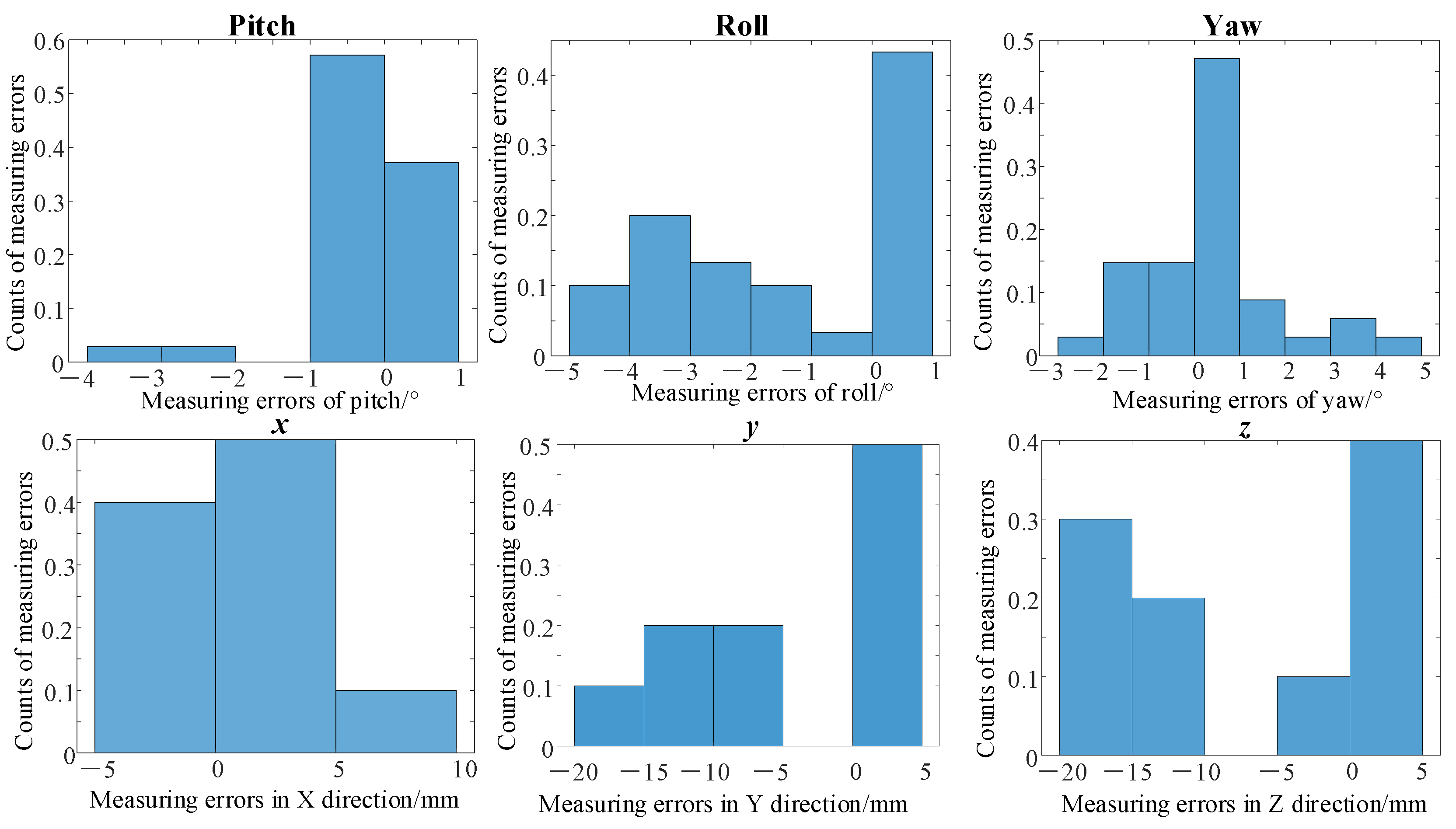
The algorithm proposed in this paper is used to estimate the pre-alignment pose between the camera and the target, and its error is calculated, as shown in Figure 11.
As can be seen from Figure 11, the position measurement errors of the pose estimation algorithm proposed in this paper are all less than 20.0 mm and the attitude angle measurement errors are all less than 2.5° in the whole measurement process, indicating that the proposed algorithm fully meets the accuracy requirements of the rendezvous and docking of the non-cooperative target spacecraft.
Moreover, the actual measurement error is greater than the simulation error because the change of the illumination environment during the measurement process leads to a large error of line extraction. Meanwhile, the system pose measurement also involves the unified process of the global coordinate system, which will introduce errors into the final structure.

5. Conclusions

In this paper, binocular stereo vision is used to obtain the 3D space straight line of a non-cooperative spacecraft. The 3D reconstruction algorithms of the spatial straight lines are used to realize the 3D feature information perception of the target. Combined with the uncertainty analysis of the straight-line reconstruction, the extraction accuracy of the feature required for the pose estimation is improved, and the robustness of the algorithm is enhanced. Finally, according to the parameters of the straight line, combined with the intersection vector algorithm and the nonlinear optimization algorithm, the position and pose solution method is derived. The simulation and actual experiments show that the algorithm proposed in this paper can accurately estimate the relative pose of the spacecraft in the ultra-short range.

Author Contributions

Conceptualization, Y.L. and X.X.; methodology, Z.M.; software, Y.L. and Y.Y.; validation, Y.L., Y.Y. and X.X.; formal analysis, Y.L.; investigation, Y.L.; resources, Y.L.; data curation, Y.Y.; writing—original draft preparation, X.X.; writing—review and editing, X.X.; visualization, Y.Y.; supervision, Y.L.; project administration, Z.M.; funding acquisition, Z.M. All authors have read and agreed to the published version of the manuscript.

Funding

This research was funded by the China Postdoctoral Science Foundation, grant number 2021M702078.

Data Availability Statement

Not applicable.

Acknowledgments

Thanks to Shanghai Agriculture and Rural Committee.

Conflicts of Interest

The authors declare no conflict of interest.

References

  1. Liang, B.; Du, X.; Li, C.; Xu, W. Advances in Space Robot On-orbit Servicing for Non-cooperative Spacecraft. ROBOT 2012, 34, 242–256. [Google Scholar] [CrossRef]
  2. He, Y.; Liang, B.; He, J.; Li, S. Non-cooperative spacecraft pose tracking based on point cloud feature. Acta Astronaut. 2017, 139, 213–221. [Google Scholar] [CrossRef]
  3. Cougnet, C.; Gerber, B.; Heemskerk, C.; Kapellos, K.; Visentin, G. On-orbit servicing system of a GEO satellite fleet. In Proceedings of the 9th ESA Workshop on Advanced Space Technologies for Robotics and Automation ‘ASTRA 2006’ ESTEC, Noordwijk, The Netherlands, 28–30 November 2006. [Google Scholar]
  4. Ibrahim, S.K.; Ahmed, A.; Zeidan, M.A.E.; Ziedan, I.E. Machine Learning Methods for Spacecraft Telemetry Mining. IEEE Trans. Aerosp. Electron. Syst. 2018, 55, 1816–1827. [Google Scholar] [CrossRef]
  5. Woods, J.O.; Christian, J.A. Lidar-based relative navigation with respect to non-cooperative objects. Acta Astronaut. 2016, 126, 298–311. [Google Scholar] [CrossRef]
  6. Fan, B.; Du, Y.; Wu, D.; Wang, C. Robust vision system for space teleoperation ground verification platform. In Proceedings of the 32nd Chinese Control Conference, Xi’an, China, 26–28 July 2013. [Google Scholar]
  7. Opromolla, R.; Fasano, G.; Rufino, G.; Grassi, M. A review of cooperative and uncooperative spacecraft pose determination techniques for close-proximity operations. Prog. Aerosp. Sci. 2017, 93, 53–72. [Google Scholar] [CrossRef]
  8. Terui, F.; Kamimura, H.; Nishida, S.I. Motion estimation to a failed satellite on orbit using stereo vision and 3D model matching. In Proceedings of the 9th International Conference on Control, Automation, Robotics and Vision, Singapore, 5–8 December 2006. [Google Scholar]
  9. Terui, F.; Kamimura, H.; Nishida, S. Terrestrial experiments for the motion estimation of a large space debris object using image data. In Proceedings of the Intelligent Robots and Computer Vision XXIII: Algorithms, Techniques, and Active Vision, Boston, MA, USA, 23–25 October 2005. [Google Scholar]
  10. Sharma, S.; Beierle, C.; D’Amico, S. Pose estimation for non-cooperative spacecraft rendezvous using convolutional neural networks. In Proceedings of the IEEE Aerospace Conference, Big Sky, MT, USA, 3–10 March 2018. [Google Scholar]
  11. Sharma, S.; D’Amico, S. Systems, Neural network-based pose estimation for noncooperative spacecraft rendezvous. IEEE Trans. Aerosp. Electron. Syst. 2020, 56, 4638–4658. [Google Scholar] [CrossRef]
  12. Du, X.; He, Y.; Chen, L.; Gao, S. Pose estimation of large non-cooperative spacecraft based on extended PnP model. In Proceedings of the 2016 IEEE International Conference on Robotics and Biomimetics (ROBIO), Qingdao, China, 3–7 December 2016. [Google Scholar]
  13. Li, Y.; Huo, J.; Yang, M.; Cui, J. Non-cooperative target pose estimate of spacecraft based on vectors. In Proceedings of the Chinese Control Conference (CCC), Guangzhou, China, 27–30 July 2019. [Google Scholar]
  14. Pan, H.; Huang, J.; Qin, S. High accurate estimation of relative pose of cooperative space targets based on measurement of monocular vision imaging. Optik 2014, 125, 3127–3133. [Google Scholar] [CrossRef]
  15. De Jongh, W.; Jordaan, H.; Van Daalen, C. Experiment for pose estimation of uncooperative space debris using stereo vision. Acta Astronaut. 2020, 168, 164–173. [Google Scholar] [CrossRef]
  16. Xu, C.; Zhang, L.; Cheng, L.; Koch, R. Pose Estimation from Line Correspondences: A Complete Analysis and a Series of Solutions. IEEE Trans. Pattern Anal. Mach. Intell. 2016, 39, 1209–1222. [Google Scholar] [CrossRef] [PubMed]
  17. Wang, P.; Xu, G.; Cheng, Y. A novel algebraic solution to the perspective-three-line pose problem. Comput. Vis. Image Underst. 2020, 191, 102711. [Google Scholar] [CrossRef]
  18. Wang, P.; Xu, G.; Cheng, Y.; Yu, Q. A simple, robust and fast method for the perspective-n-point Problem. Pattern Recognit. Lett. 2018, 108, 31–37. [Google Scholar] [CrossRef]
  19. Mirzaei, F.M.; Roumeliotis, S.I. Globally optimal pose estimation from line correspondences. In Proceedings of the IEEE International Conference on Robotics and Automation, Shanghai, China, 9–13 May 2011. [Google Scholar]
  20. Li, X.; Zhang, Y.; Liu, J. A direct least squares method for camera pose estimation based on straight line segment correspondences. Acta Opt. Sin. 2015, 35, 0615003. [Google Scholar]
  21. Liu, Y.; Xie, Z.; Zhang, Q.; Zhao, X.; Liu, H. A new approach for the estimation of non-cooperative satellites based on circular feature extraction. Robot. Auton. Syst. 2020, 129, 103532. [Google Scholar] [CrossRef]
  22. He, Y.; Zhao, J.; Guo, Y.; He, W.; Yuan, K. PL-VIO: Tightly-Coupled Monocular Visual–Inertial Odometry Using Point and Line Features. Sensors 2018, 18, 1159. [Google Scholar] [CrossRef] [PubMed] [Green Version]
  23. Cui, J.; Li, Y.; Huo, J.; Yang, M.; Wang, Y.; Li, C. A measurement method of motion parameters in aircraft ground tests using computer vision. Measurement 2021, 174, 108985. [Google Scholar] [CrossRef]
  24. Wang, Y. Research on Motion Parameters Measuring System based on Intersected Planes. Harbin Inst. Technol. 2015. Available online: https://kns.cnki.net/KCMS/detail/detail.aspx?dbname=CMFD201601&filename=1015982210.nh (accessed on 18 September 2022).
  25. Cui, J.; Min, C.; Feng, D. Research on pose estimation for stereo vision measurement system by an improved method: Uncertainty weighted stereopsis pose solution method based on projection vector. Opt. Express 2020, 28, 5470–5491. [Google Scholar] [CrossRef] [PubMed]
  26. Zhang, Z. A flexible new technique for camera calibration. IEEE Trans. Pattern Anal. Mach. Intell. 2000, 22, 1330–1334. [Google Scholar] [CrossRef]
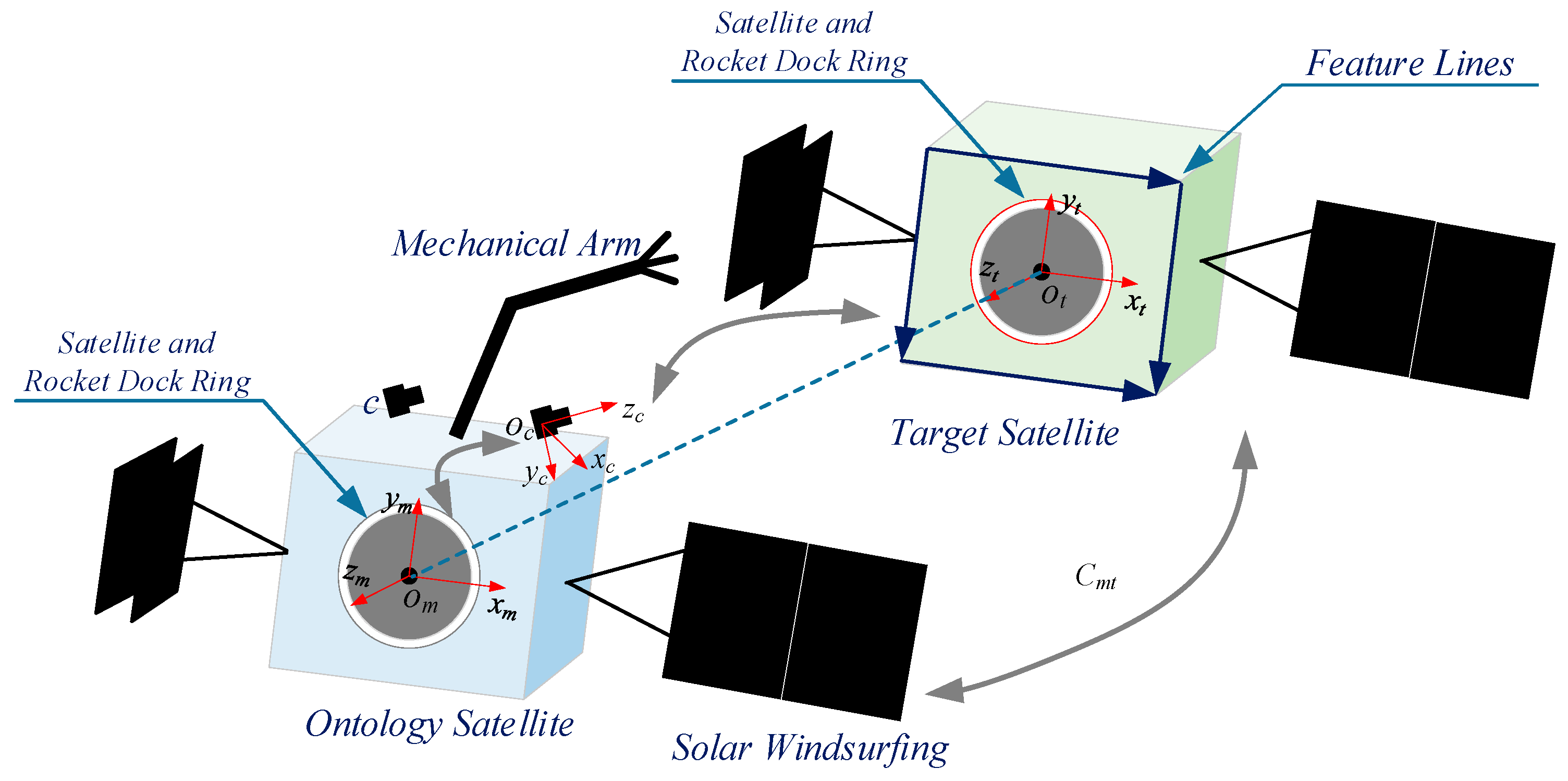
Figure 1. Schematic diagram of the relative pose estimation of a non-cooperative spacecraft.
Aerospace 09 00681 g001
Figure 2. Schematic diagram of the spatial straight-line perspective projection imaging.
Aerospace 09 00681 g002
Figure 3. Uncertainty analysis of the straight lines.
Aerospace 09 00681 g003
Figure 4. Schematic diagram of the straight-line distance error analysis.
Aerospace 09 00681 g004
Figure 5. Schematic diagram of the linear distance representation in the different coordinate systems.
Aerospace 09 00681 g005
Figure 6. Flow chart of the outer space non-cooperative target pose estimation algorithm.
Aerospace 09 00681 g006
Figure 7. Pose estimation accuracy at the different measurement frequencies. (a) Attitude measurement error at 10 Hz; (b) Position measurement error at 10 Hz; (c) Attitude measurement error at 2.5 Hz; (d) Position measurement error at 2.5 Hz.
Aerospace 09 00681 g007
Figure 8. Statistics of the measurement accuracy of the different algorithms. (a) Attitude measurement error; (b) Position measurement error.
Aerospace 09 00681 g008
Figure 9. The influence of the different image measurement noise levels on the measurement accuracy of the algorithm. (a) Attitude measurement error; (b) Position measurement error.
Aerospace 09 00681 g009
Figure 10. Non-cooperative target motion acquisition images.
Aerospace 09 00681 g010
Figure 11. Non-cooperative target poses solution results.
Aerospace 09 00681 g011
Table 1. Simulation parameter setting of the target motion.
Position/mmPose/°
txtytzYawRollPitch
10 sin(0.2πt)525 t10 sin(0.2πt)10 sin(0.2πt)10 sin(0.2πt)10 sin(0.2πt)
Table 2. Calibration results of the binocular vision.
External parameterBaseline/mm1224.98
rotate/°(120.92, −14.55, −27.04)
Intrinsic parameterradial distortion l,r(−0.219, 0.072)(−0.240, 0.129)
focal l,r/mm(10.37, 10.37)(10.37, 10.37)
principal point l,r/mm(5.84, 5.47)(5.48, 5.63)
Table 3. Statistics of the static pose estimation experimental results.
Average ErrorMaximum Error
Rotation Error (°)Translation Error (mm)Rotation Error (°)Translation Error (mm)
Feature Point method1.229.352.7525.85
Visual Odometry method5.5115.154.8555.38
Direct Linear method1.3012.122.5839.25
Proposed method1.199.242.3518.74
Publisher’s Note: MDPI stays neutral with regard to jurisdictional claims in published maps and institutional affiliations.