Research on the Prediction Problem of Satellite Mission Schedulability Based on Bi-LSTM Model

Abstract

The realization of microsatellite intelligent mission planning is the current research focus in the field of satellite planning, and mission schedulability prediction is the basis of this research. Aiming at the influence of the sequence tasks before and after the task sequence to be predicted, we propose an online schedulability prediction model of satellite tasks based on bidirectional long short-term memory (Bi-LSTM) on the basis of describing and establishing the satellite task planning and solving model. The model is trained using satellite offline mission planning data as learning samples. In the experiment, the prediction effect of the model is excellent, with a recall rate of 93.17% and a precision rate of 92.59%, which proves that the model can be effectively applied to predict the schedulability of satellite tasks.

1. Introduction

Imaging satellites mainly use payloads such as on-board optical equipment or radio equipment to observe ground, sea or air targets and obtain target information on the orbit. Imaging satellites have shown great roles and potentials in both military operations and civilian applications [1]. With the continuous development of satellite technology and the continuous improvement of on-board load technology, users’ demands for satellites are also increasing. We need to improve the ability to rationally allocate limited satellite resources to maximize the satisfaction of users’ needs within a limited time. Satellite mission planning refers to a technology that reasonably allocates satellite resources and formulates action sequences to optimize the execution of satellite observation missions according to user needs. Satellite mission planning plays a key role in the entire Earth observation process.

Existing studies have shown that satellite mission planning is a typical non-deterministic polynomial hard (NP-hard) problem [2]. At present, the research ideas for solving this problem are mainly based on the mode of “mission description, model construction, algorithm solution, evaluation and optimization”. The construction of the model and the solution of the algorithm are the key points, and there are many research results corresponding to it. In addition, the basic process used to solve the task planning problem is to first analyze the actual requirements and constraints of the plan, then establish the corresponding framework model, and solve the algorithm for each module in the framework model, and finally the task execution sequence is obtained from the ground and uploaded to the satellite to complete the entire satellite observation mission planning.

However, the ever-changing space operating environment, changing satellite status, and changing user needs pose great challenges to the existing mission planning technology. At the same time, the vigorous development of artificial intelligence technology has also brought new development directions for mission planning technology. In order to meet the needs of complex earth observation missions, the development and application of imaging satellite mission planning are gradually developing in the direction of collaboration, intelligence and online functions. The premise and basis of satellite intelligent mission planning is that satellites can intelligently decide whether a certain mission needs to be executed and whether it can be executed. In order to solve this problem, the concept of mission schedulability has been proposed in the field of satellite planning. Task schedulability also predicts the execution of any observation task in the observation task sequence based on the task execution capabilities of different satellites, the current task loads of different satellites, and the earth observation requirements provided by users.

At present, the research on the schedulability prediction of imaging satellite tasks is still in its infancy. Thinker et al. [3] first proposed a method for predicting the schedulability of satellite tasks based on case learning, using historical satellite planning data sets for unsupervised learning, and comparing with known examples to complete satellite task prediction. Li et al. [4] used the classic machine learning method decision tree and support vector machine to achieve task schedulability prediction, which proved the effectiveness of the method. With the development of machine learning, Bai Guoqing [5], Liu Song [6], Xing Lining [7] and others proposed to use back propagation (BP) neural networks to predict the schedulability of satellite tasks, which improved the prediction effect, but this method ignores the learning of the temporal features of the observation task. In this regard, Peng et al. [8] proposed a task schedulability prediction method based on the long short-term memory (LSTM) model, which takes the task sequence as the input, realizes the forward and backward transfer of task timing characteristics, and further improves the prediction accuracy.

This paper proposes a Bi-LSTM-based imaging satellite observation task schedulability prediction model, which predicts whether the input task sequence is executable or not. This method can effectively model the potential interaction between the before and after observation tasks, so as to realize the accurate prediction of the schedulability of multiple observation tasks at one time, and output the task sequence that can be directly executed. The rest of the paper is organized as follows. The second section describes and analyzes the task scheduling prediction problem mathematically. The third section describes the Bi-LSTM model and its solution in detail. The fourth section provides experimental verification and comparative analysis. The last section concludes with a summary and future research directions.

2. Problem Description and Analysis

The online task schedulability prediction problem of imaging satellites can be described as: through the supervised learning of historical planning data of satellite tasks, the mapping relationship between task execution and constraints is simulated, so as to realize the function of predicting the input task sequence. The key elements of the problem will be analyzed below.

2.1. Input and Output of Task Scheduling Prediction Problem

The input of the task scheduling prediction problem is a task sequence with unknown execution results, and the input task sequence is defined as$\mathrm{X}=\left\{x_1,x_2, \dots , x_i, \dots ,x_N\right\}$, where N is the number of pre-input tasks to be executed. The output task set obtained after the task sequence is predicted by the model is defined as $\mathrm{Y}=\left\{y_1, y_2, \dots , y_i, \dots , y_N\right\}$, where $y_i$ indicates whether task $x_i$ is executed,

$$y_i=\left\{\begin{array}{c}0 ,task x_i is not executed\\ 1 ,task x_i is executed\end{array}\right.$$

(1)

2.2. Constraint Analysis

In the constraint analysis, this paper mainly considers the constraints of the task itself, and reasonably simplifies the actual constraints such as orbital maneuverability and side sway of the satellite itself. Based on the observation of point targets by imaging satellites, the following constraints are considered.

• Satellite Time Window Constraints

A satellite can only perform one task at a time, and only one of the multiple observable time windows of the same task needs to be selected. The start time of the time window of the satellite to perform task $x_i$ is $Wi{n}_{S_i}$, the end time is $Wi{n}_{E_i}$, and the time window can be expressed as $Win=\left(Wi{n}_{S_i}, Wi{n}_{E_i}\right)$. The relationship between any two different task time windows of the task sequence is shown in Figure 1 below.

As shown in the figure, there are a total of four temporal relations between the time windows of the execution of two adjacent satellite missions. Among them, only the first time window relation can satisfy the temporal constraint, and the mathematical expression of this relation can be expressed as:

$$\left(y_{i}Wi{n}_{S_i}-y_{j}Wi{n}_{E_j}\right)\left(y_{i}Wi{n}_{E_i}-y_{j}Wi{n}_{S_j}\right) \ge 0$$

(2)

2.

Power Constraint

In this paper, we only consider the energy consumption of satellite actions during the execution of a certain sequence task, and the satellite does not have the energy replenishment function temporarily during the execution of the task. When the satellite performs task $x_i$, the on-board power consumption of the satellite is $B_{x_i}$, and the upper limit of the power consumption during the satellite execution task is $B_{max}$. $B_{max}$ represents the total amount of power allocated by the power system during the execution of a sequence of tasks. The power consumption satisfies the constraint expression:

$${\displaystyle \sum }_{i=1}^n{y}_i{B}_{x_i}\le B_{max}$$

(3)

3.

Storage Constraints

When the satellite performs task $x_i$, the on-board storage occupied is $D_{x_i}$, the maximum on-board storage is $D_{max}$, and the occupied storage satisfies the constraints:

$${\displaystyle \sum }_{i=1}^n{y}_i{D}_{x_i}\le D_{max}$$

(4)

2.3. Optimization Objective

In this paper, the optimization objective of task prediction is defined as maximizing the profit of the task execution sequence under the condition that all constraints are satisfied, so the profit obtained after the execution of task $x_i$ is defined as $P_{x_i}$. The total profit of task execution is:

$$Y=\mathit{max}{\displaystyle \sum }_{i=1}^n{y}_i{P}_{x_i}$$

(5)

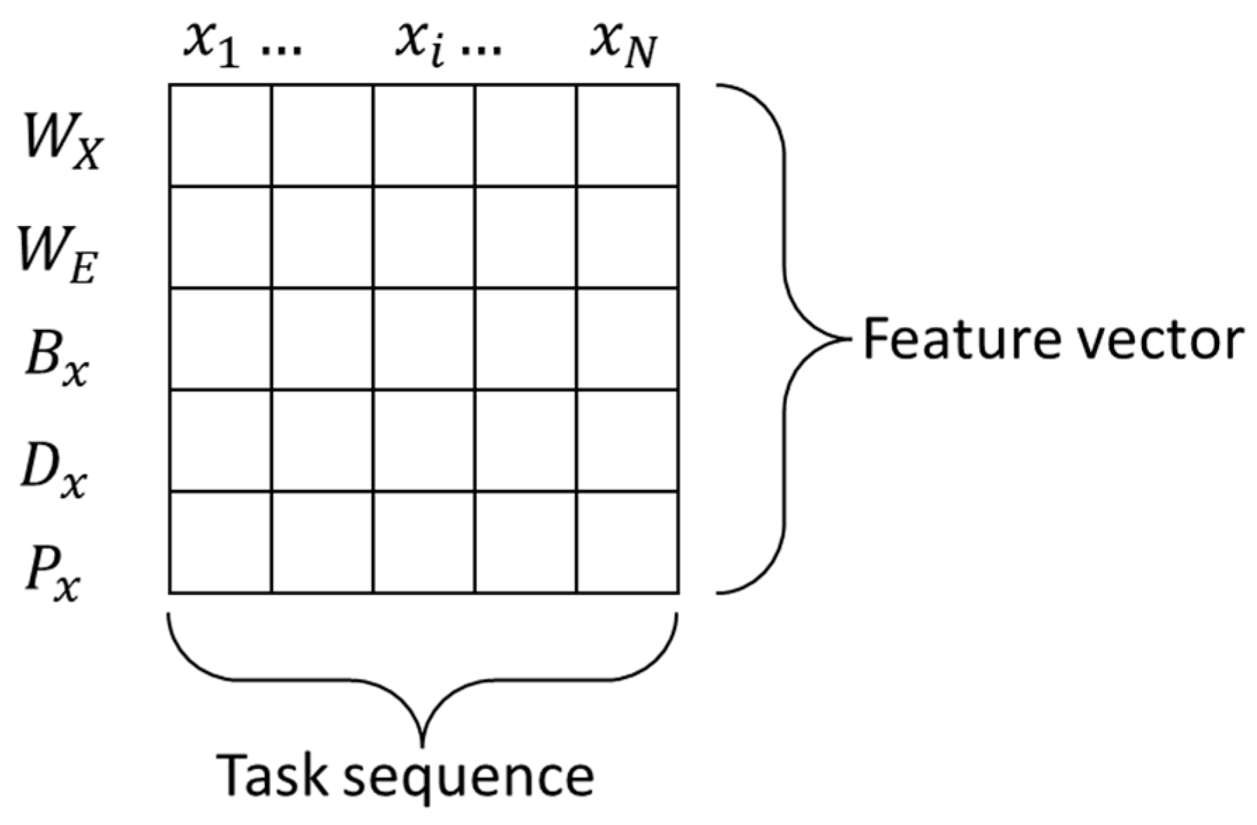
Taking the above conditions into consideration, this paper selects the task start time, end time, power consumption, storage occupancy, and task profit as the characteristic attribute input of the observation task set X.

3. Model Analysis

3.1. Introduction to Bi-LSTM

Long short-term memory (LSTM) is a type of recurrent neural network in deep learning that takes sequence data as input, performs recursion in the evolution direction of the sequence, and all nodes (recurrent units) are connected in a chain.

Due to the long-term dependency problem of the basic RNN model, scholars have proposed long short-term memory [9], a specific form of recurrent neural network, which can effectively overcome the gradient vanishing problem in RNN, especially in long-distance-dependent tasks, which is far better than RNN [10].

For a given input sequence $\mathrm{X}=\left\{x_1, x_2, \dots , x_N\right\}$, using a standard RNN model for training, as shown in Figure 2, a hidden layer sequence $H=\left\{h_1, h_2, \dots , h_N\right\}$ and a final output sequence $\mathrm{Y}=\left\{y_1, y_2, \dots , y_N\right\}$ can be computed. $W_x$, $W_y$ and$W_h$in the figure represent the weight matrix of each layer of the model.

LSTM is a variant optimization model of RNN; the basic structure is similar to RNN [11] and the difference is that LSTM implements a more refined internal processing unit. As shown in Figure 3, there are three important gates in the LSTM unit, namely: input gate, forget gate and output gate [12].

Gating can be regarded as a fully connected layer, and it is in these gates that LSTM stores and updates information. The general form of gating can be expressed as:

$$g\left(x\right)=\sigma \left(Wx+b\right)$$

(6)

Among them, $\sigma \left(x\right)=1/\left(1+\mathit{exp}\left(-x\right)\right)$ is called the Sigmoid function [13], which is a nonlinear activation function commonly used in machine learning, which can map a real value to the interval 0–1 to describe how much information passes through. When the output value of the gate is 0, it means that no information passes through, and when the value is 1, it means that all information can pass through.

We use $i$, $f$ and $o$ to denote the input gate, forget gate and output gate, and W and b to denote the weight matrix and bias vector of the network. The forward calculation process of LSTM can be expressed as Equations (7)–(11). At time step t, the input and output vectors of the hidden layer of the LSTM are $x_t$ and $h_t$, and the memory cell is $c_t$. The input gate is used to control how much of the current input data $x_t$ of the network flows into the memory unit, that is, how much can be saved to $c_t$, and its value is:

$$i_t=\sigma \left(W_{xi}{x}_t+W_{hi}{h}_{t-1}+b_i\right)$$

(7)

The forget gate is a key component of an LSTM cell that controls which information is kept and which is forgotten, and somehow avoids the vanishing and exploding gradient problems that arise when the gradients backpropagate over time. It controls the self-connecting unit and can decide which parts of the historical information will be discarded. That is, the influence of the information in the memory unit $c_{t-1}$ at the previous moment on the current memory unit $c_t$.

$$f_t=\sigma \left(W_{xf}{x}_t+W_{hf}{h}_{t-1}+b_f\right)$$

(8)

$$c_t=f_t{c}_{t-1}+i_t\mathit{tan}h\left(W_{xc}{x}_t+W_{hc}{h}_{t-1}+b_c\right)$$

(9)

The output gate controls the influence of the memory unit on the current output value $c_t$, that is, which part of the memory unit will output at time step t. The value of the output gate is shown in Equation (10), and the output of the LSTM unit at time t can be obtained by Equation (11).

$$o_t=\sigma \left(W_{xo}{x}_t+W_{ho}{h}_{t-1}+b_o\right)$$

(10)

$$h_t=o_t\mathit{tan}h\left(c_t\right)$$

(11)

In order to make the prediction results more accurate, Schuster M [14] et al. proposed a bidirectional recurrent neural network based on the recurrent neural network, which contains a forward LSTM layer and a backward LSTM layer, and the forward state and the backward state are connected in an output layer. During the training process, the model is trained in both forward and backward directions, which effectively solves the problem that the LSTM model ignores the impact of future input on the output.

3.2. Model Construction

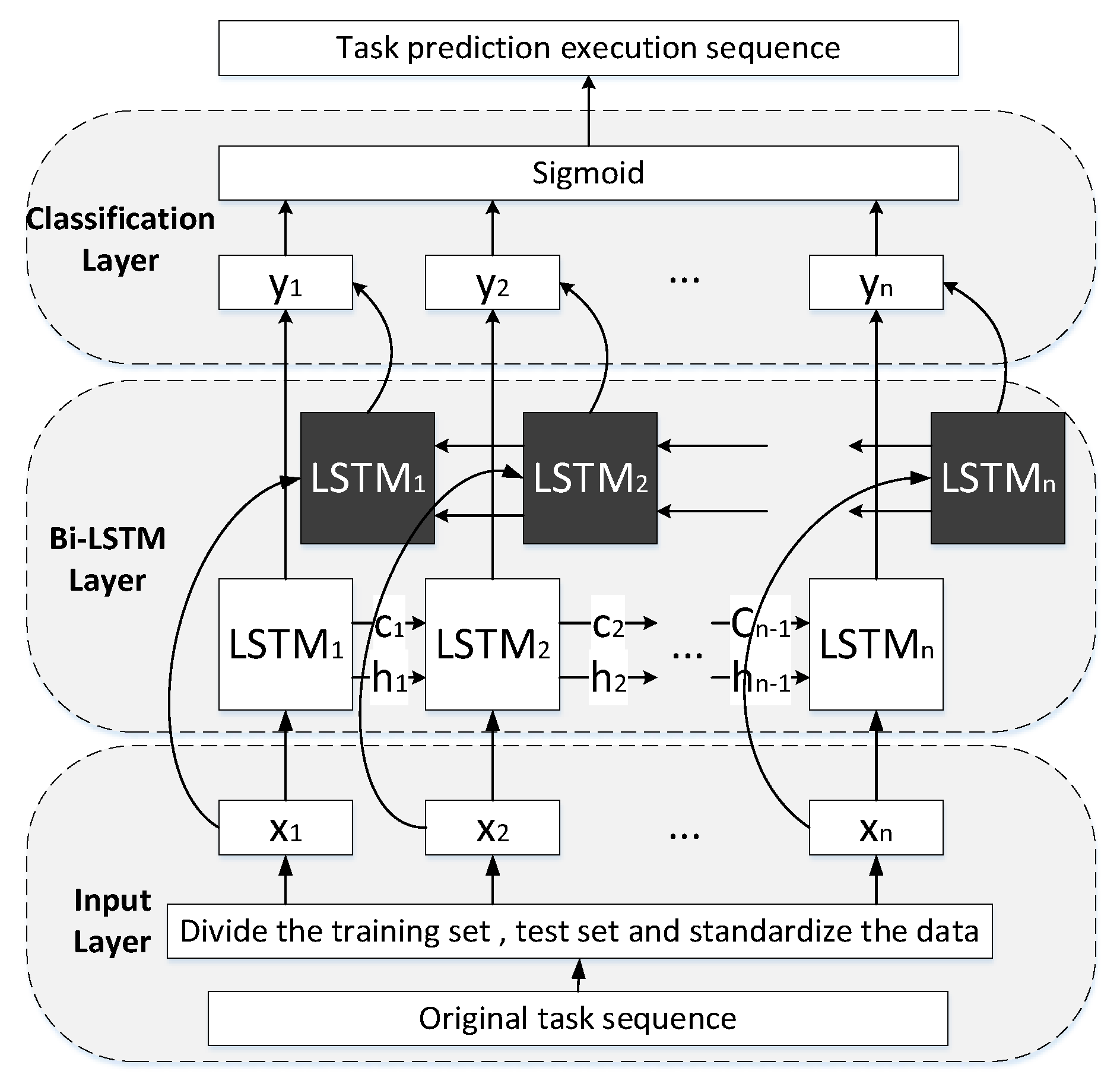
As shown in the Figure 4, this paper establishes a Bi-LSTM network-based satellite online task schedulability prediction problem model. The model consists of an input layer, a Bi-LSTM layer and a classification layer.

• Input Layer

The input layer performs data standardization processing and data set division on the original task sequence, thereby obtaining an N × 5-dimensional feature input matrix that meets the network input requirements, as shown in Figure 5 below.

2.

Bi-LSTM layer

As shown in Figure 4, the Bi-LSTM layer consists of a forward LSTM and a backward LSTM. Both consist of N LSTM units. The forward LSTM is mainly used to obtain the features of the previous task sequence, and the reverse LSTM is mainly used to obtain the features of the future task sequence. In addition, both the forward and reverse LSTM encode the input at the current moment. The state calculation formula of the forward LSTM unit is:

$${\overrightarrow{h}}_t=f\left(\overrightarrow{W}\left[{\overrightarrow{h}}_{t-1},x_t\right]+\overrightarrow{b}\right)$$

(12)

The state calculation formula of the reverse LSTM unit is:

$${\overleftarrow{h}}_t=f\left(\overleftarrow{W}\left[{\overleftarrow{h}}_{t-1},x_t\right]+\overleftarrow{b}\right)$$

(13)

Among them, the variables with → in the superscript all represent the calculation process in the forward unit, and the variables with ← in the superscript represent the calculation process in the reverse calculation unit. $h_t$ represents the state of the hidden layer at the current time t, and $h_{t-1}$ represents the state of the hidden layer at the previous time. $x_t$ represents the value input into the cell at time t, and b represents the bias. Finally, the combined output is passed to the classification layer.

3.

Classification Layer

The classification layer composed of the fully connected layer maps the output of the hidden layer to the predicted probability, using the Sigmoid function, and the calculation formula is:

$$P\left(y|X\right)=Sigmoid\left(f\left(W\left[\overrightarrow{h},\overleftarrow{h}\right]+b\right)\right)$$

(14)

where f is the ReLU activation function, and W and b are the weight matrix and bias vector, respectively.

3.3. Model Training

In order to train the established model, this paper adopts cross entropy [15] to calculate the loss. In the model, the loss function is:

$$Loss=-\frac{1}{N}{\displaystyle \sum }_{i=1}^{M}p\left(y,X_N\right)\ln P(y|X_N)$$

(15)

The effect of the Bi-LSTM prediction model is affected by the hyperparameter settings, which requires parameter optimization. In this paper, the Adam optimization algorithm is selected to obtain the optimal solution that minimizes the loss function. The Adam optimization algorithm is an extension of the stochastic gradient descent algorithm that has recently been widely used in deep learning applications [16].

The specific model training process is shown in the pseudo code of Algorithm 1:

Algorithm 1 Model training process pseudo-code

Input: Traindata/I Output: ${\omega }_{best}$ 1. Initialize i 2. $\mathrm{Initialize} \omega$ 3. $Sample=⟨X, Y⟩=\left\{⟨x_1, y_1⟩, \dots , ⟨x_n, y_n⟩\right\}$  4. $Y^{\prime 0}\leftarrow Bi-LSTM\left(\left.X\right|{\omega }^0\right)$ 5. $L^0\leftarrow \frac{1}{n}{\displaystyle \sum }_{j=1}^n Loss\left(\left.Y,Y^{\prime 0}\right|X,{\omega }^0\right)$ 6. for i = 1, …, I do 7.    $g\leftarrow {\nabla }_{\theta }{\displaystyle \sum }_{j=1}^n Loss\left(\left.Y, Y^{\prime i-1}\right|X,{\omega }^{i-1}\right)$ 8.    $\Delta \omega \leftarrow Adam\left(\left.g\right|X,{\omega }^{i-1}\right)$ 9.    ${\omega }^i\leftarrow {\omega }^{i-1}+\Delta \omega$ 10.   $Y^{\prime i}\leftarrow Bi-LSTM\left(\left.X\right|{\omega }^i\right)$ 11.   $L^i\leftarrow \frac{1}{n}{\displaystyle \sum }_{j=1}^{n}Loss\left(\left.Y, Y^{\prime i}\right|X, {\omega }^i\right)$ 12.    $\mathrm{if}Min\left(L^0, \dots , L^{i-1}\right)\succ L^i$ $\mathrm{then} {\omega }_{best}\leftarrow {\omega }^i$ 13.    end if 14. end for

Among them, the input of the model is the training data set Traindata and the total number of training iterations I, and steps 1–2 initialize the iteration count parameter i. Step 3 selects sample data from the training data set, and steps 4–5 use the initialized parameters to calculate the initialized prediction result $Y^{\prime 0}$ and the average loss function value $L^0$ of the sample data. Steps 6–14 perform gradient calculation, model parameter update, prediction result update, and average loss function value update on the model, save the model parameters whose loss function takes the minimum value, and repeat the above steps until the iteration cycle ends.

4. Experiment and Analysis

4.1. Experimental Environment and Experimental Data

• Experimental hardware environment

The experimental code is written in Python language on the PyCharm compiler, and the Keras open-source artificial neural network library is used. The experimental computer is configured with Intel(R) Core (TM) i7-8750H CPU @ 2.20 GHz, running memory is 8.0 GB, and the operating system is Windows 10.

2.

Experimental data preparation

The data used in this experiment are the simulation data. Using MATLAB and STK co-simulation, with the conditions mentioned in Section 2.2 of this paper as constraints, the genetic algorithm is used to solve the execution result of the satellite task sequence, that is, the data set label of the Bi-LSTM model. Genetic algorithm is a method to obtain historical planning data. Set the simulation time as 00:00:00 on 1 April 2017 to 23:59:59 on 1 April 2017. The research object of this paper is the prediction of single-star mission executability, so the experimental object is a visible light imaging satellite with an orbital altitude of 1500 km. The target points are evenly set on 30 latitudes of the earth, and a total of 566 target points are set. As long as the satellite can establish a link with a certain target, it is considered that the task between the satellite and the target point can be executed, that is, the time window for establishing the link is the time window of the task. All tasks in the experiment are earth observation tasks. When the Earth observation satellite is carrying out its mission, it consumes the electricity provided by the power system. After the mission is completed, the imaging results occupy the on-board storage space. The experimental data consist of 5000 sets of observation task sequences, of which 75% are used for training the neural network and 25% are used for testing.

4.2. Model Parameter Settings

In order to make the model prediction more accurate, in the process of experimenting with different sets of data, the LSTM layer in the model, the number of layers of the fully connected layer and the number of hidden nodes of the LSTM are debugged respectively. When the final number of LSTM layers is set to 2, the number of fully connected layers is set to 2, and the number of hidden nodes of the LSTM layer is set to 32, the model has the highest prediction accuracy, and the prediction accuracy reaches 92.59%.

4.3. Evaluation Criteria and Model Results

In order to evaluate the experimental performance of the model, this paper selects prediction models such as one-way LSTM model and Gated recurrent unit (GRU) as the baseline for performance comparison. Both LSTM and GRU are classical distortions of RNN. We use loss value, accuracy, and ROC curve to evaluate the above models.

Figure 6 shows the loss value and accuracy of the training results of the Bi-LSTM model proposed in this paper. The loss value is the distance between the model output and the true result, defined using cross-entropy as the loss function. Accuracy refers to the frequency that the predicted results in the model are consistent with the actual labels. The calculation expression is:

$$Accuracy=\frac{TP+TN}{P+N}$$

(16)

where P is the number of positive samples, N is the number of negative samples, TP is the number of positive samples predicted to be positive by the model, TN is the number of negative samples predicted to be negative by the model.

It can be seen from the figure that in the task prediction of the test set, the accuracy rate reaches 92.59%, and the prediction performance is excellent. In the early stage of training, the model performs better than the test set on the training set. After a large amount of training of the model, the test performance of the model reaches the training effect.

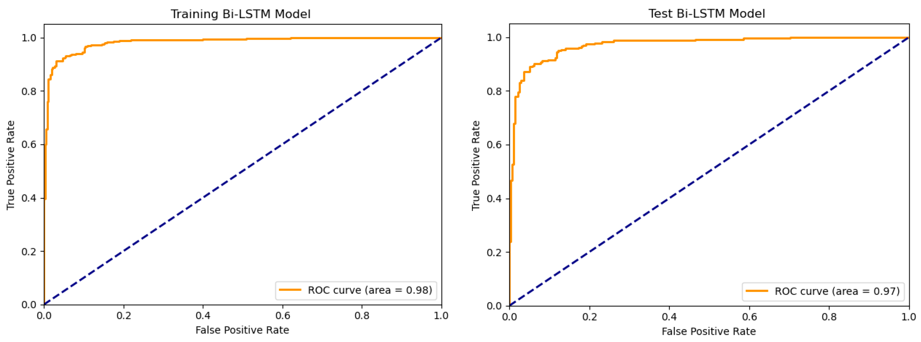
Figure 7 shows the training and testing ROC curves of the model proposed in this paper. The ROC curve is the relationship between the probability of being correctly predicted in the actual positive sample and the probability of being incorrectly predicted as a positive sample in the actual negative sample. As can be seen from the figure, the ROC curve is convex to the upper left, which indicates that the model predicts well.

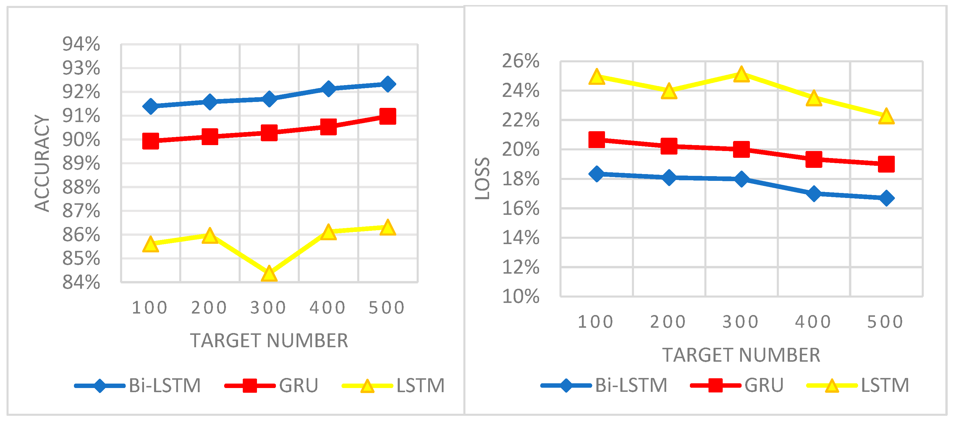
In order to verify the excellent performance of the proposed model, this paper sets 5 different scenarios with different observation target points, and uses GRU, LSTM, and Bi-LSTM models to predict task schedulability under 100, 200, 300, 400, and 500 target observation points, respectively. The model performance comparison is shown in Figure 8 below.

It can be seen from the figure that the precision of the BI-LSTM model is higher than that of the GRU and LSTM models in different scenarios, with the highest being 1.6% higher than the GRU model and 7.32% higher than the LSTM model. Therefore, the model performs better in terms of prediction accuracy, and is more suitable for solving the schedulability prediction problem of satellite observation tasks. At the same time, it can be seen that, to a certain extent, the more observation targets, the more tasks in the task sequence, the more the neural network Bi-LSTM model is trained, and the more accurate the results are.

5. Conclusions and Outlook

This paper proposes a Bi-LSTM-based satellite online task prediction problem model. After training the model with a large amount of offline satellite mission planning data, the real-time prediction function of satellite online schedulable tasks can be realized. The model fully considers the influence of adjacent or even distant tasks before and after the prediction task, and can simultaneously predict all tasks in a task sequence at one time. The experiment also conducted a comparison test of similar models, and the model performed better in terms of recall, precision and F1 value. Mission executability prediction is the foundation of satellite onboard intelligent mission planning. The method proposed in this paper can better realize the function of task execution prediction. Therefore, this method will be useful in subsequent research.

This paper is aimed at predicting the schedulability of single-satellite missions. Future research can focus on the following aspects:

• To establish a multi-satellite task schedulable prediction model, use multi-satellite offline planning data for training, and realize the multi-satellite online task schedulable prediction function.
• To establish a satellite mission planning model on the basis of realizing the prediction function, further plan the prediction results, and realize the optimal planning of the mission under the condition of adding constraints such as the greatest benefit and the shortest planning time.
• When considering the constraints of satellite missions, this paper makes certain simplifications. In practical applications, all realistic constraints need to be considered to further improve the model.

References

1. Jun, J. Survey of remote sensing imaging observation technology. Northeast. Surv. Mapp. 2000, 23, 7–8. [Google Scholar]
2. Bensana, E.; Verfaillie, G.; Agnese, J.C.; Bataille, N.; Blumstein, D. Exact and Inexact Methods for the Daily Management of an Earth Observation Satellite; European Space Agency: Paris, France, 1996. [Google Scholar]
3. Tinker, P.; Fox, J.; Green, C.; Rome, D.; Casey, K.; Furmanski, C. Analogical and Case-Based Reasoning for Predicting Satellite Task Schedulability. In Proceedings of the International Conference on Case-based Reasoning Research & Development, Chicago, IL, USA, 23–26 August 2005; Springer: Berlin/Heidelberg, Germany, 2005. [Google Scholar]
4. Li, J.; Jing, N.; Hu, W.; Chen, H. A satellite schedulability prediction algorithm for EO SPS. Chin. J. Aeronaut. 2013, 26, 705–716. [Google Scholar] [CrossRef] [Green Version]
5. Bai, G.-Q.; Chen, Y.-W.; Yang, Z.-Y.; Liu, S. Prediction Method of Imaging Satellite Mission Schedulability Based on Integrated BP Neural Network; Chinese Academy of Astronautics; Institute of Electronics, Chinese Academy of Sciences: Beijing, China, 2013. [Google Scholar]
6. Song, L.; Bai, G.-Q.; Chen, Y.-W. A method for predicting the schedulability of earth observation network imaging tasks. Chin. J. Astronaut. 2015, 36, 583–588. [Google Scholar]
7. Xing, L.; Wang, Y.; He, Y.; He, L. Prediction method of onboard mission schedulability based on BP neural network. China Manag. Sci. 2015, S1, 117–124. [Google Scholar]
8. Peng, S.; Chen, H.; Du, C.; Li, J.; Jing, N. Onboard Observation Task Planning for an Autonomous Earth Observation Satellite Using Long Short-Term Memory. IEEE Access 2018, 6, 65118–65129. [Google Scholar] [CrossRef]
9. Hochreiter, S.; Schmidhuber, J. Long short-term memor. Neural Comput. 1997, 9, 1735–1780. [Google Scholar] [CrossRef] [PubMed]
10. Gers, F.A.; Schmidhuber, J.; Cummins, F. Learning to Forget: Continual Prediction with LSTM; Istituto Dalle Molle Di Studi Sull Intelligenza Artificiale: Viganello, Switzerland, 1999. [Google Scholar]
11. Bayer, J.; Wierstra, D.; Togelius, J.; Schmidhuber, J. Evolving memory cell structures for sequence learning. In Proceedings of the International Conference on Artificial Neural Networks, Limassol, Cyprus, 14–17 September 2009; Springer: Berlin/Heidelberg, Germany, 2009; pp. 755–764. [Google Scholar]
12. Graves, A.; Fernández, S.; Schmidhuber, J. Bidirectional LSTM networks for improved phoneme classification and recognition. In Proceedings of the International Conference on Artificial Neural Networks, Warsaw, Poland, 11–15 September 2005; Springer: Berlin/Heidelberg, Germany, 2005; pp. 799–804. [Google Scholar]
13. Zhang, Y.; Qu, L. Unipolar Sigmoid neural network classifier based on weights and structure determination method. J. Comput. Appl. 2013, 33, 766. [Google Scholar] [CrossRef]
14. Schuster, M.; Paliwal, K.K. Bidirectional recurrent neural networks. IEEE Trans. Signal Process. 1997, 45, 2673–2681. [Google Scholar] [CrossRef]
15. Martinez, M.; Stiefelhagen, R. Taming the cross entropy loss. In Proceedings of the German Conference on Pattern Recognition, Stuttgart, Germany, 9–12 October 2018; Springer: Cham, Switzerland, 2018; pp. 628–637. [Google Scholar]
16. Kingma, D.P.; Ba, J. Adam: A method for stochastic optimization. arXiv 2014, arXiv:1412.6980. [Google Scholar]
Figure 1. Time window relationship diagram.
Aerospace 09 00676 g001
Figure 2. Recurrent neural network structure.
Aerospace 09 00676 g002
Figure 3. LSTM model structure.
Aerospace 09 00676 g003
Figure 4. Bi-LSTM predictive model structure.
Aerospace 09 00676 g004
Figure 5. Input matrix.
Aerospace 09 00676 g005
Figure 6. Loss and accuracy of training results.
Aerospace 09 00676 g006
Figure 7. Bi-LSTM model ROC curve.
Aerospace 09 00676 g007
Figure 8. Model performance comparison.
Aerospace 09 00676 g008
Publisher’s Note: MDPI stays neutral with regard to jurisdictional claims in published maps and institutional affiliations.