Remaining Useful Life Prediction for Aero-Engines Based on Time-Series Decomposition Modeling and Similarity Comparisons

Abstract

The aero-engine is the heart of an aircraft; its performance deteriorates rapidly due to the high temperature and high-pressure environment during flights. It is necessary to predict the remaining useful life (RUL) to improve the reliability of aero-engines and provide security for reliable flights. In previous flights, the sensors collected a lot of performance parameter data and formed a database regarding the aero-engine degradation process. These performance parameters cannot reflect the degradation process directly. In this paper, fuzzy clustering is applied to divide the degradation stages of the aero-engine, construct the health indicator, and describe the degradation process. Time-series decomposition modeling is applied to predict the degradation process of the health indicator. Based on the idea of similarity comparison, the RUL is predicted by comparing the similarity of time series through example learning. The method is verified and analyzed on the dataset published by National Aeronautics and Space Administration (NASA), and the mean square error (MSE) is 528. The result is better than the comparative method.

1. Introduction

As the core component of the aircraft, the aero-engine is always in extremely high temperatures, pressure and a high-frequency vibration environment during its work. And the aero-engine is shown in Figure 1. In this environment, the functions of various components of the engine continue to deteriorate with time, and the remaining useful life (RUL) also decreases. It is difficult for the engine with degraded functions to perform its tasks well, and sometimes the degradation even causes serious consequences. Therefore, for a long time, scientific researchers have been studying and putting forward the prediction methods of the RUL of aero-engines.

At present, the RUL prediction methods are mainly divided into three categories: (1) methods based on physical failure models; (2) data-driven models; (3) a mixed model of the above two methods [1]. The method based on the physical failure model combines the prior knowledge of the component composition, working principle and degradation mechanism of the equipment with the sensor detection data to build a physical or mathematical model to characterize the function degradation process of the equipment, thus, predicting the RUL of the aero-engine, such as the Paris Erdogan model [2], the nonlinear cumulative damage model [3] and the Wiener random process model [4]. This prediction method has high accuracy, but its model is not universal and the modeling process is complex. The data-driven method mines the health status information and degradation law of equipment from the monitoring data, and then builds the mapping relationship between the monitoring data and RUL. Although the prediction accuracy of this technology is not as high as that of the physical degradation model, it is more versatile and flexible to use. The hybrid model is an organic combination of two methods, such as the combination of the exponential regression model and correlation vector machine [5]. This method cannot avoid the problem that the physical regression model is difficult to establish. Therefore, the data-driven model is the most commonly used RUL prediction method.

In practical applications, data-driven degradation prediction methods can be di-vided into two categories: (1) machine-learning prediction models biased towards statistical learning; (2) machine-learning prediction models biased towards deep learning. In academic circles, it is generally believed that statistical learning and traditional machine learning are essentially the same two concepts. Both of them study the information contained in the data, but statistical learning pays more attention to interpretation, while traditional machine learning pays more attention to prediction. Statistical learning is the machine learning of computer systems to improve the system performance by using data and statistical methods [6]. In statistical learning, it is assumed that similar data have certain statistical regularity. Therefore, the machine-learning prediction model for prediction biased towards statistical learning establishes a statistical model based on empirical knowledge according to health monitoring data containing the health degradation information [7]. Zaidan et al. [8] introduced the deterministic approximation of Bayesian inference into the general two-level hierarchical linear model, assuming the conjugate prior distribution for engine predictions. Liu et al. [9,10] proposed a parametric p-order polynomial model and verified it on the degradation dataset of an aircraft gas turbine engine. Statistical methods are also widely used in multivariate regression modeling and predictions. Cui et al. [11] used the fast DTW method to improve the speed-of-similarity calculation, obtain the best classification results by searching the optimal hyperparameter K of K-Nearest Neighbor, and extract the effective features in turn. In [12], the fault time and multisensor data are combined by a novel potential linear model to construct a general health indicator (HI). In order to improve the accuracy of a real-time RUL prediction during a system operation, Zhang et al. [13] proposed a real-time RUL modeling method based on the adaptive kernel window width density. In this method, the kernel density estimation of known samples recursively updates the kernel density estimation of samples with the real-time changes of monitoring data. The machine-learning prediction model biased towards statistical learning can establish the degradation model of the system without massive data and has good universality, thus, the research is very extensive.

Deep learning is a superset of machine learning. Deep learning deepens the hidden layer, with large parameters and weak interpretability. It is like a "black box". Its model is built on data and is more dependent on data. Therefore, the feature of machine-learning prediction models biased towards deep learning is that it requires a large amount of data and can automatically extract features and construct models based on massive data for the RUL prediction. For example, the deep belief network (DBN) or the DBN-based fusion model proposed in [14,15,16] is used to automatically extract useful features from raw data. The convolutional neural network (CNN) is also applied to mechanical RUL predictions because of its strong feature extraction ability, parameter sharing and excellent characteristics of partial network parallelism [17]. Jiao et al. [18] used the recurrent neural network (RNN) to extract features to estimate health indicators (HI) and predict the RUL of the system. For a small-sample RUL prediction, Fu et al. [19] proposed a prediction method using data augmentation (DA) and a deep bidirectional gate recursive unit (DBGRU), and Cui et al. [20] designed the prediction model based on the sliding window and grey neural network. Han et al. [21] used the online transfer learning method to transfer knowledge under different conditions to improve the accuracy of RUL predictions. More methods integrate different deep learning models and learn from each other to improve the prediction accuracy, such as the combination of LSTM and RNN [22]; the combination of CNN and superimposed bidirectional and unidirectional LSTM networks [23]; the combination of the one-dimensional convolutional neural network (1D-CNN) and bidirectional long- and short-term memory (Bi-LSTM) [24]; and the combination of CNN, timing convolutional neural networks (TCN), and multi-head attention mechanism [1]. Although the machine-learning prediction model biased towards deep learning can extract deeper features, its interpretability is poor. Because it relies too much on data, the accuracy of its prediction may also decrease when the training data changes. Therefore, at present, the machine-learning prediction models biased towards statistical learning have stronger usability and higher research values.

This paper presents an RUL prediction method based on time-series decomposition modeling and similarity measurements, which belong to the machine-learning prediction model biased towards statistical learning. The multi-dimensional monitoring performance parameters of aero-engines contain a lot of engine health information. The degradation process can be divided into different degradation stages through fuzzy clustering, and can construct HI based on clustering results. Aero-engines have accumulated a lot of HI degradation tracks. Through the similarity measurement method, high similarity segments can be matched from the degradation track database, and the RUL prediction can be completed with dynamic weight. Considering that the degradation trajectory only reflects the degradation condition of the aero-engine running to the current state, the degradation trajectory is predicted by time-series decomposition modeling by introducing the predictive similarity measurement method. The method is verified and analyzed on the dataset published by NASA (National Aeronautics and Space Administration), and the mean square error (MSE) is 528. The result is better than the comparative test. The prediction results have safety bias, which provides a strong support for aero-engine health management.

The following chapters are arranged as follows: Section 2 explains the relevant basic theories of the proposed method for the convenience of later understanding. In Section 3, the proposed method is described in detail, and the implementation of the algorithm is introduced. In Section 4, the algorithm verification and comparison tests are carried out based on the dataset published by NASA. Section 5 summarizes this paper.

2. Preliminaries

2.1. Fuzzy C-Means (FCM)

2.1.1. Basic Principles

Cluster analysis refers to the process of applying mathematical methods to classify things according to their similarities. In traditional clustering analysis, because of the properties of each set, it is a hard division with clear boundaries. However, in reality, many analysis objects do not have strict attributes, that is, the relationship between them has fuzzy characteristics [25,26,27]. Traditional hard clustering analysis cannot be used to study these objects with fuzzy relations, and the fuzzy set theory provides a tool for the distinction of objects with unclear boundaries [28,29]. Fuzzy clustering analysis generally has the following steps. Firstly, construct the fuzzy matrix according to the attributes of the research object. Secondly, determine the clustering relationship according to a certain degree of membership. This method quantitatively determines the fuzzy relationship between samples with the method of fuzzy mathematics to cluster objectively and accurately.

2.1.2. Computational Steps

Fuzzy C-means is mainly divided into the following steps:

(1)

Define clustering objects.

Let the universe $U={[u_1,u_2,\cdots ,u_n]}^T$ be a space with n samples, each ${\mathit{u}}_i$ sample has m features, namely ${\mathit{u}}_i=\left[x_{i1},x_{i2},\cdots ,x_{im}\right](i=1,2,\cdots ,n)$, so the original data matrix is

$$\mathit{U}=\left[\begin{array}{c}{\mathit{u}}_1\\ {\mathit{u}}_2\\ ⋮\\ {\mathit{u}}_n\end{array}\right]=\left[\begin{array}{cccc}{x}_{11}& x_{12}& \cdots & x_{1m}\\ x_{21}& x_{22}& \cdots & x_{2m}\\ ⋮& ⋮& & ⋮\\ x_{n1}& x_{n2}& \cdots & x_{nm}\end{array}\right]$$

(1)

where $x_{nm}$ is the original data of the mth feature of the nth classification object.

(2)

Data standardization.

In practical problems, the dimensions of data are generally different, thus, it is necessary to deal with the data in dimensions so that they can be compared with each other. Here, the data standardization regards transforming the data into the interval [0, 1] to meet the requirements of the fuzzy matrix. Data standardization usually includes translation standard deviation transformation, translation range transformation and logarithmic transformation. In this paper, the maximum and minimum normalization method is used for standardization. The formula is:

$$x_{ik}^{″}=\frac{x_{ik}^{\prime }-\underset{1⩽i⩽n}{min}\left\{x_{ik}^{\prime }\right\}}{\underset{1⩽i⩽n}{max}\left\{x_{ik}\right\}-\underset{1⩽i⩽n}{min}\left\{x_{ik}{}^{\prime }\right\}}$$

(2)

where $k=1,2,\cdots ,m,i=1,2,\cdots ,n$.

(3)

Eablish fuzzy similarity matrix.

The fuzzy similarity matrix constructed from the original data is an important basis for later clustering, and the correctness of clustering depends entirely on this matrix. At present, there are 13 methods to construct the fuzzy similarity matrix, including the Hamming distance method, Euclidean distance method, Chebyshev distance method, included angle cosine method, maximum and minimum method, etc. [30]. According to the research, the selection of the fuzzy similarity matrix construction method should follow the following three principles: correctness principle, invariability principle and distinguishability principle. After making a comprehensive comparison of 13 fuzzy similarity matrix construction methods, the maximum and minimum method is most suitable for constructing the fuzzy similarity matrix. In this paper, the maximum and minimum method is selected to construct the fuzzy similarity matrix, and the calculation formula is:

$$\mathit{R}=\left\{r_{ij}\right\},r_{ij}=\frac{{\displaystyle \sum _{k=1}^m}\left(x_{ik}\wedge x_{jk}\right)}{{\displaystyle \sum _{k=1}^m}\left(x_{ik}\vee x_{jk}\right)}$$

(3)

where ∧ is the operation of “taking the small”; ∨refers to the “larger” operation.

(4)

Clustering.

Common clustering analysis methods include the direct clustering method based on the fuzzy similarity matrix, the clustering method based on fuzzy clustering equivalence (transfer closure method, Boolean matrix method) and the fuzzy clustering analysis method based on objective functions. The first two methods can receive the classification of each measurement unit under different thresholds through calculation, but the second method is more mature, while the third method generally needs to determine the number of clusters before calculation. Considering the actual situation, this paper adopts the FCM fuzzy clustering algorithm in the third one. FCM algorithm does not need human intervention in the process of algorithm implementation. It is an unsupervised data clustering method based on the optimization of the objective function. The clustering result is the membership degree of each data point to the clustering center, which is expressed by a numerical value. The algorithm allows the same sample to belong to multiple different classes.

The objective function is:

$$\begin{array}{ll}\min J_{FCM}\left(U,V\right)& ={\displaystyle \sum _{k=1}^C}{\displaystyle \sum _{k=1}^N}{u}_{ki}^m‖x_i-v_k‖{}^2\\ \mathrm{s.}\mathrm{t.}{\displaystyle \sum _{k=1}^N}{u}_{ki}& =1,u_{ki}\in \left[0,1\right]\end{array}$$

(4)

where C is the number of clusters and N is the number of samples. U is the membership matrix and V is the cluster center.

(5)

Determine the optimal threshold λ.

Select different thresholds in clustering λ, and different classifications can be obtained. The higher λ is, the greater the number of classifications is, and vice versa [31]. In practical problems, we need to choose the appropriate one λ to determine the number of clusters of samples, and generally use an empirical method and F statistics to determine the best threshold λ.

①

Empirical method: The threshold is adjusted by several experienced experts according to the actual situation λ to select the appropriate classification number.

②

F statistics: Assume that the threshold is λ when the number of classifications is r and the number of samples is n, the F statistic follows the F distribution with degrees of freedom of r−1 and n−r, and the formula of F statistic is

$$F=\frac{{\displaystyle \sum _{j=1}^r}{n}_j‖{\overline{\mathit{u}}}^{\left(j\right)}-\overline{\mathit{u}}‖{}^2/\left(r-1\right)}{{\displaystyle \sum _{i=1}^r}{\displaystyle \sum _{j=1}^{n_j}}‖{\mathit{u}}_i^{\left(j\right)}-{\overline{\mathit{u}}}^{\left(j\right)}‖{}^2/\left(n-r\right)}$$

(5)

where the molecule represents the distance between different classes; the denominator represents the distance between samples within the class. The larger the value of the F statistic, the smaller the difference within the class and the larger the difference between classes, that is, the better the classification effect. At the significant level α, if F > F α (r−1, n−r), according to the statistical principle, it is reasonable to classify under this significant level, therefore, the difference between different classes is significant.

2.2. Seasonal Trend Decomposition Procedure Based on LOESS (STL)

The seasonal trend decomposition procedure based on LOESS (STL) was first proposed by Cleveland et al. [32] to decompose the time-series data of the monthly atmospheric carbon dioxide concentration. At present, many scholars use STL to decompose time-series data (such as UCR) to obtain more valuable information in time-series data [33].

For a given time series Y(t), STL can decompose it into three additive components: trend component T(t), seasonal component S(t), and residual component R(t), namely:

$$Y(t)=T(t)+S(t)+R(t)$$

(6)

Among them, the seasonal component S(t) refers to the cyclical component (such as 12 months, 4 quarters, etc.). STL contains two nested cycles—inner cycle and outer cycle. In the inner cycle, the trend component T(t) and seasonal component S(t) are mainly extracted through LOESS. In the outer loop, the residual component R(t) is calculated, and the sample robust weight Pr is calculated according to the residual component to reduce the influence of outliers on the smoothing result of LOESS.

First, assume that the number of cycles of the inner cycle is $i=1,2,\dots ,$ I and initialize the trend component: $T^{\left(0\right)}\left(t\right)=0$. For each inner cycle, there are the following six steps:

Step 1: Remove the trend component. By subtracting the trend component $T^{\left(i-1\right)}\left(t\right)$ obtained from the previous cycle from the original sequence Y(t), the time series ${\tilde{T}}^{\left(i\right)}\left(t\right)$ of de trend is obtained, i.e.:

$${\tilde{T}}^{(i)}(t)=Y(t)-T^{(i-1)}(t),t=1,2,\dots ,T$$

(7)

Step 2: Periodic subsequence smoothing. Extract periodic subsequences from ${\tilde{T}}^{\left(i\right)}\left(t\right)$; then, use loess $\mathrm{LOESS}\left(K_1\right)$ to smooth each periodic subsequence, and extend one cycle forward and one cycle backward at the same time. Then, arrange these periodic subsequences in chronological order to form sequence $C^{\left(i\right)}\left(t\right)$. Note that the length of time series here extends from T to T + 2L.

Step 3: Low channel filtering. Make three moving averages of length L (i.e., one cycle length), L, and 3 for Sequence $C^{\left(i\right)}\left(t\right)$ in turn, and finally use $\mathrm{LOESS}\left(K_2\right)$ smoothing to obtain sequence $E^{\left(i\right)}\left(t\right),t=1,2,\dots ,N$. Note that the length of time series here changes from $T+2L$ of $C^{\left(i\right)}\left(t\right)$ to T of $E^{\left(i\right)}\left(t\right)$.

Step 4: Calculate seasonal components. Calculate the seasonal component $S^{\left(i\right)}\left(t\right)$ according to the following formula:

$$S^{(i)}(t)=C^{(i)}(t)-E^{(i)}(t),t=1,2,\dots ,T$$

(8)

Step 5: Remove seasonal ingredients. Subtract the seasonal component $S^{\left(i\right)}\left(t\right)$ from the original sequence $Y\left(t\right)$ to obtain the time series ${\tilde{S}}^{\left(i\right)}\left(t\right)$ without seasonal components:

$${\tilde{S}}^{(i)}(t)=Y(t)-S^{(i)}(t),t=1,2,\dots ,T$$

(9)

Step 6: Calculate the trend component. Use $\mathrm{LOESS}\left(K_3\right)$ to smooth the seasonal component ${\tilde{S}}^{\left(i\right)}\left(t\right)$ and get the trend component $T^{\left(i\right)}\left(t\right)$.

When the above six steps are completed, the trend component T(t) and seasonal component S(t) can be obtained.

In the external circulation, first calculate the residual component R(t) according to the following formula:

$$R(t)=Y(t)-T(t)-S(t)$$

(10)

The residual component R(t) is used to reflect the abnormal deviation of the original data. When the residual component at time t is large, it indicates that the abnormal condition of the sample is serious, which will affect the smoothing effect of loess in the internal circulation process. In order to solve this problem, the sample robust weight ${\rho }_t$ is introduced. Due to the influence of correcting outliers, the calculation formula of ${\rho }_t$ is as follows:

$${\rho }_t=\mathrm{B}\left(\frac{R(t)}{6\times \mathrm{median}(|R(t)|)}\right)$$

(11)

where, $B(t)=\left\{\begin{array}{c}{\left(1-t^2\right)}^2,\left|t\right|\le 1\\ 0,\mathrm{others}\end{array}\right.$, median$\left(\left|R\left(t\right)\right|\right)$ represents the median of the absolute value of the residual component R(t). After obtaining the robust weight of all samples, in the next inner loop, all the LOESS smoothing processes in steps 2 to 6—after finding the adjacent points—multiply the value of the adjacent points by the robust weight ${\rho }_t$. From the above formula, it can be seen that when the residual component R(t) of the sample at time t is large, the robust weight ${\rho }_t$ of the sample is smaller. When $R\left(t\right)\ge 6 median\left(\left|R\left(t\right)\right|\right)$, the robust weight of the sample is ${\rho }_t$= 0, thus, indicating that this point will not be considered in the process of loess smoothing.

When the outer cycle also ends, three decomposition components of the original sequence Y(t) can be obtained: the trend component T(t), the seasonal component S(t) and the residual component R(t).

3. Proposed Methods

3.1. RUL Predictions Based on STL Modeling and Similarity Measurements

The overall framework for RUL predictions based on STL modeling and similarity comparisons is shown in Figure 2. The method is divided into two modules: offline degradation trajectory database construction, and online degradation trajectory modeling and RUL prediction. The offline module includes two parts: preprocessing and HI construction. The online module includes three parts: HI prediction, degradation trajectory prediction and RUL prediction.

In the offline stage, data preprocessing, feature selection and feature extraction are carried out. Additionally, fuzzy clustering is employed to divide the degradation stage and construct HI. The aero-engine monitoring data have different types and magnitudes. In order to facilitate the subsequent calculation and processing, the minimum and maximum normalization is used for standardization.

$$x_i^{*}=\frac{x_i-x_{\min }}{x_{\max }-x_{\min }}, i\in 1, 2,\cdots , n$$

(12)

For high-dimensional monitoring data, the features should be selected through the statistics method. In this paper, filter feature selection is used for its strong versatility and simple calculation. The statistics and correlation coefficients of each dimensional feature are used as the evaluation criteria to select a feature subset with better performance. The main criteria include variance, Pearson coefficient and Spearman’s coefficient.

$$D(X)=E{(X_t-\overline{X})}^2={\displaystyle {\sum }_{i=1}^n{(x_i-\overline{X})}^2}$$

(13)

$$r_p=\frac{{\displaystyle \sum _{i=1}^n\left(x_i-\overline{x}\right)\left(y_i-\overline{y}\right)}}{\sqrt{{\displaystyle \sum _{i=1}^n{\left(x_i-\overline{x}\right)}^2}}\sqrt{{\displaystyle \sum _{i=1}^n{\left(y_i-\overline{y}\right)}^2}}}$$

(14)

where $\overline{x}$ and $\overline{y}$ are the mean value of X and Y, respectively.

$$r_s=\frac{{\displaystyle \sum _{i=1}^n\left(r_i-\overline{r}\right)\left(s_i-\overline{s}\right)}}{\sqrt{{\displaystyle \sum _{i=1}^n{\left(r_i-\overline{r}\right)}^2}}\sqrt{{\displaystyle \sum _{i=1}^n{\left(s_i-\overline{s}\right)}^2}}}$$

(15)

where $r_i$ and $s_i$ are the ranks of $x_i$ and $y_i$, respectively.

The dimension after feature selection is still high. In order to facilitate fuzzy clustering and better observe the clustering effect, PCA is used for feature extraction. After data preprocessing, the performance data obtained by feature extraction at different times are clustered by fuzzy clustering. The degradation process is divided into health stage, degradation stage and near-failure stage, and the clustering center point is obtained. Taking the cluster center as the evaluation benchmark, combined with the performance data at each time, the health degree is measured by distance. The HI transformation model is designed to construct the historical degradation trajectory database of an aero-engine.

The online stage includes the health prediction of online data, degradation modeling and degradation trajectory prediction of single engines based on STL decomposition, and RUL prediction based on similarity comparison. For online data, the membership degree of the health stage is predicted by the clustering center of historical data, and then the transformation of HI is completed. Through STL decomposition, the degradation trajectory is decomposed into trend term, seasonal term and random term. The trend item is modeled by the Autoregressive Integrated Moving Average model (ARIMA); the random term is generated by kernel density estimation (KDE) and acceptance-rejection sampling. The three items are modeled and predicted, respectively, then added to complete the prediction of degradation trajectory. The degradation trajectories of HI contain noise, and moving average filtering is used to smooth the trajectories. By comparing the similarity between the measurement segment and sliding window of historical trajectories, several segments in the historical database that are closest to the online track are selected, and the RUL is obtained by the dynamic weighting prediction.

3.2. HI Construction Based on Fuzzy Clustering

The degradation process of an aero-engine is a continuous process. It can be divided into the health stage, degradation stage and near-failure stage. In the health stage, the engine is in good health and runs smoothly, and the user does not need to carry out special treatment. In the degradation stage, the components’ performance begins to degenerate due to dynamic load and other factors. The users need to regularly observe its running state, but the engine can still run normally and complete the task. In the near-failure stage, the internal parts of the engine are near fatigue failure, and the engine can run but there is a risk of shutdown. Users need to pay close attention or replace components to ensure normal use. Figure 3 shows each degradation stage of an aero-engine.

Figure 4 shows the algorithm of HI construction based on fuzzy clustering, including fuzzy clustering, degradation stage division, health state assessment, HI transformation, etc.

The performance parameters obtained by feature extraction have a certain spatial position relationship with the change in the degradation stage. The input data are two-dimensional time series X.

$$X_{N\times 2}=\left(\begin{array}{l}{x}_1\\ x_2\\ \cdots \\ x_N\end{array}\right),x_i\in {\mathrm{R}}^2$$

(16)

Through the FCM fuzzy clustering algorithm, the number of clusters is set as three categories, and the clustering center matrix C and membership matrix U are obtained.

$$\left\{\begin{array}{l}C=\left(\begin{array}{l}{c}_1\\ c_2\\ c_3\end{array}\right)\\ U=\left(\begin{array}{ccc}{u}_{11}& \cdots & u_{1N}\\ u_{21}& \ddots & u_{2N}\\ u_{31}& \cdots & u_{3N}\end{array}\right)\end{array}\right.$$

(17)

Among them, C is composed of three cluster centers ($\mathrm{i}=1,2,3$), and U represents the membership degree data to the cluster center.

According to the membership degree to the three stages, each time corresponds to the three stages to complete the division of degradation. To satisfy the definition of HI, this paper selects the clustering center in the health stage as the benchmark and denotes it as $\hat{\mathrm{c}}$.

After the benchmark is selected, the distance between current state and the benchmark is calculated, and each engine will obtain a health-state change curve. In the whole degradation process, the health-state change curve should show an upward trend.

$$D_i=\sqrt{{(x_i-\widehat{c})}^2}, i=1, 2,\cdots , q$$

(18)

where $q$ represents the flight cycles of an aero-engine.

In order to make the HI meet the relevant definitions, the distance measurement results obtained are transformed into the health degree represented by the values in the [0, 1] interval. The conversion expression between its distance to the benchmark and the HI is as follows:

$$HI=1-\frac{D_i-D_{\min }}{D_{\max }-D_{\min }}$$

(19)

3.3. Degradation Path Prediction Based on STL Decomposition

The degradation trajectory of an aero-engine only represents the health-state in the historical flight process. In order to make the life prediction based on similarity more for-ward-looking and predict RUL in a safer way, the degradation path prediction based on STL modeling is introduced. Through STL decomposition, the original trajectory is decomposed into three parts: the trend term representing the overall degradation trend, the seasonal term representing engine characteristics, and the random term representing dynamic characteristics. Different methods are used for accurate modeling of degradation, and multi-step prediction is used to predict HI in the future. For the trend item, the ARIMA model is used for modeling and multi-step predictions. For the seasonal term, Fast Fourier Transformation (FFT) is used and the frequency with high-energy proportion is extracted for the inverse transformation to model the seasonal term. For the random item, the probability density function is obtained by KDE, and the random items are generated by acceptance-rejection sampling. The algorithm is shown in Figure 5.

The trend term reflects the historical health-state changes of an aero-engine. Since its amplitude is the largest, trend term modeling is also the most important part in the three terms, which largely determines the prediction accuracy. The ARIMA (p, d, q) model is an extension of the ARMA (p, q) model. It is widely used in time-series modeling and predictions for stationary no white noise series data. It can be expressed as

$$\left(1-\sum _{i=1}^p{\varphi }_i{L}^i\right){(1-L)}^d{X}_t=\left(1+\sum _{i=1}^q{\theta }_i{L}^i\right){\epsilon }_t$$

(20)

where $L$ is the lag operator, $d\in Z^{+}$.

The seasonal term contains some noise, and removing the noise can better reflect the seasonal information caused by the driving operation. FFT is one of the most basic methods in time domain to frequency domain transform analysis. FFT is an optimized discrete FT algorithm. The frequency spectrum of the original periodic signal can be obtained by FFT. Filtering the weak frequency can effectively extract important seasonal information and complete the seasonal-term modeling.

There are strong random terms in the degradation process, but the random terms still obey certain statistical laws. Without losing generality, the probability distribution of the random term can be obtained by estimating the kernel density of the random term. In the process of prediction, the discrete distribution is obtained by acceptance–rejection sampling from the distribution, and the random term is generated. Finally, the modeling and prediction results of the three items are added to complete the degradation path prediction.

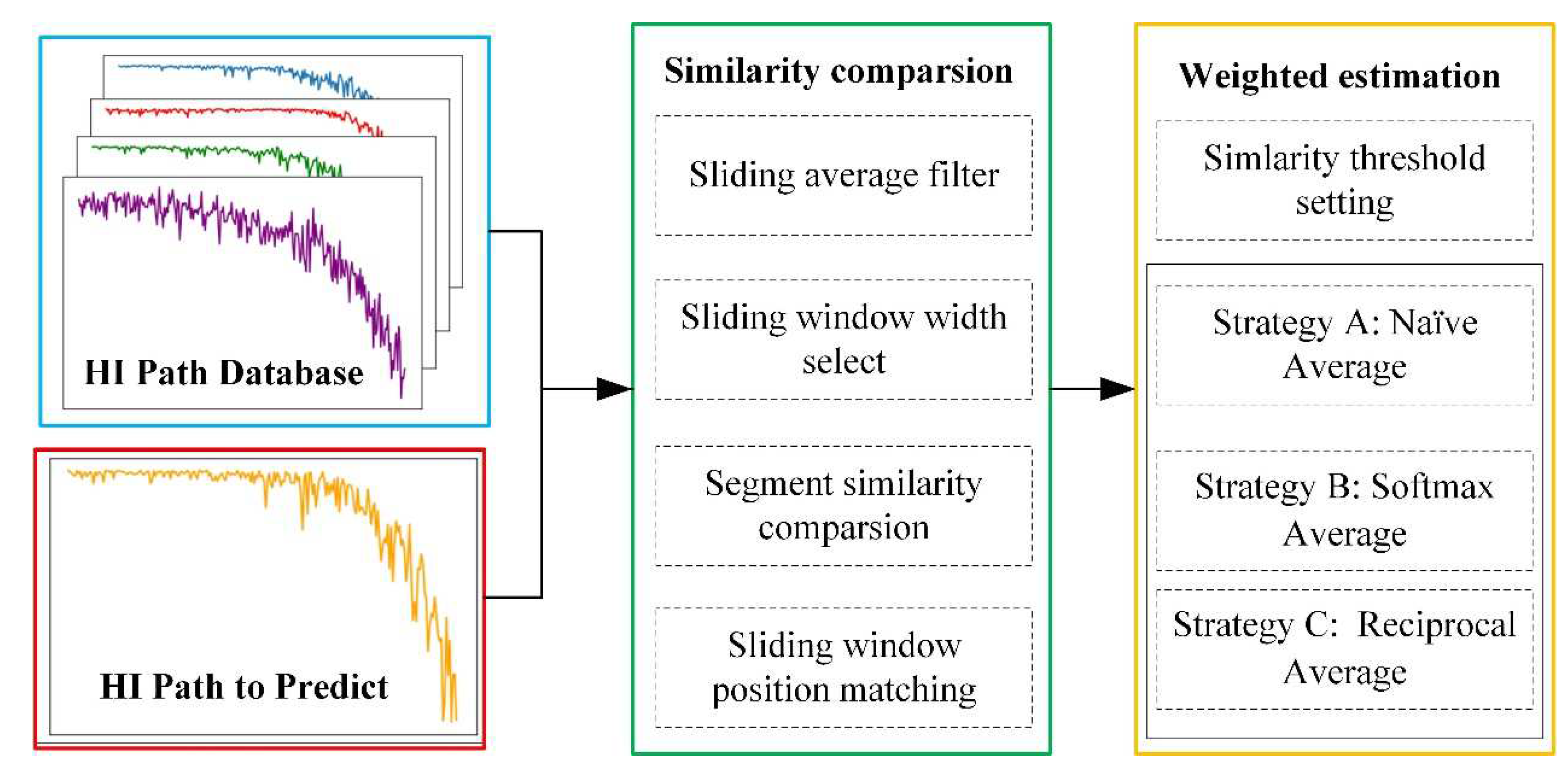
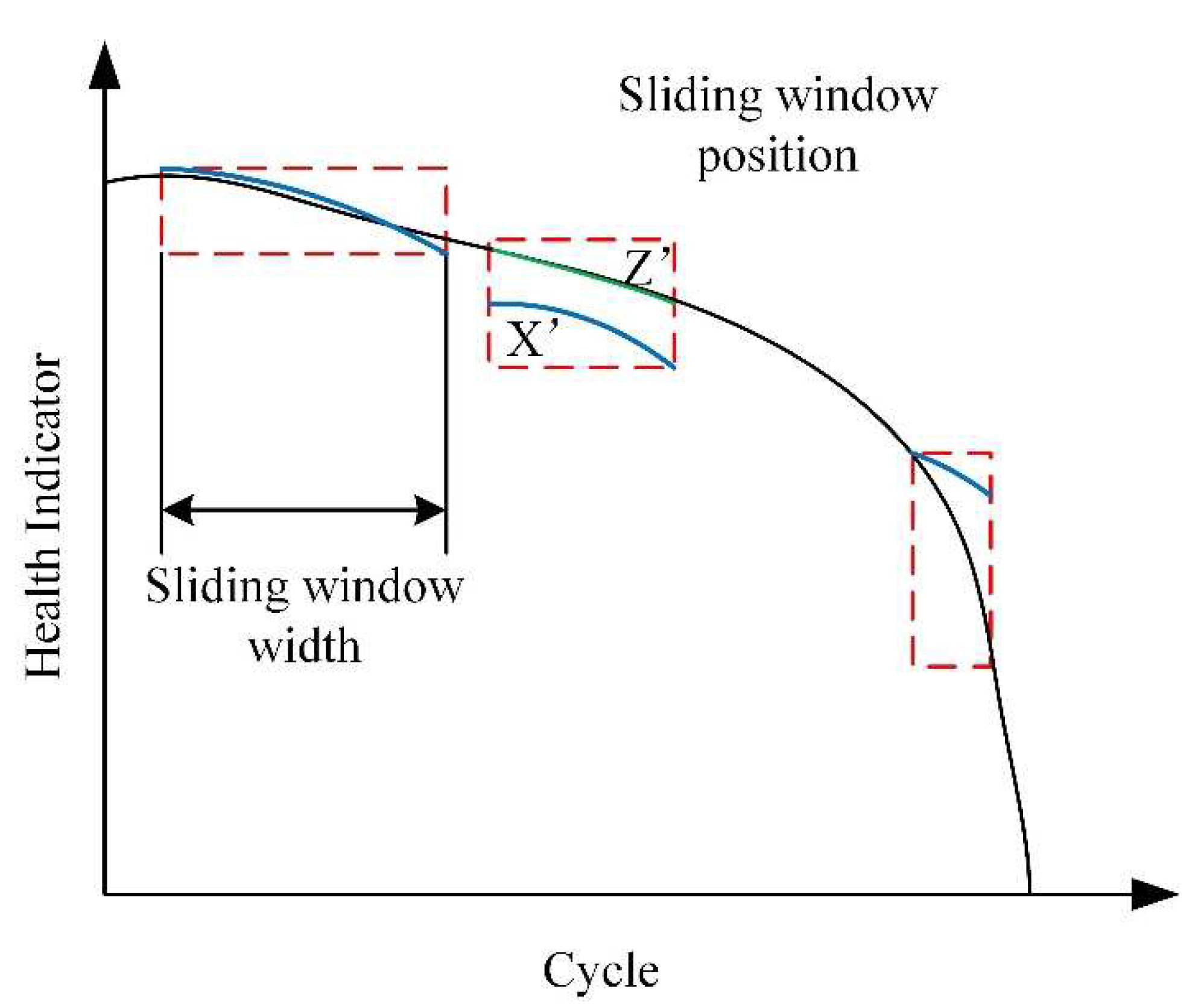
3.4. RUL Prediction Based on Similarity Comparison

As a piece of equipment with long-term service and a complete monitoring sensor, the aero-engine has a lot of history data. The life prediction method based on trajectory similarity is an example learning method. The naive modeling assumption is that similar performance degradation segments have similar RUL. As shown in Figure 6, the overall framework of the algorithm includes two main steps: trajectory similarity measurement and the weighted combination of RUL. This method does not need to establish a complex prediction model and takes the health assessment results as the input. The more cases accumulated, the stronger the generalization performance of the method. In order to improve the prediction ability of the model and reduce the risk of exceeding the actual life, the prediction results of the time-series decomposition modeling are added to the observed degradation trajectory.

Due to the noise fluctuation in the degenerate trajectory, the moving average filtering method is used to smooth the degenerate trajectory, and the boundary symmetric continuation method is used to solve the problem of boundary smoothing.

There are $X=\left\{x_1,x_2,\dots ,x_m\right\}$ degradation trajectories to be predicted with a length of m, and there are historical degradation trajectories $\left\{Y_1,\dots ,Y_i,\dots ,Y_n\right\}$, whose lengths are $q_1, q_2,\cdots , q_n$, respectively.

As shown in Figure 7, select the segment at the end of the degradation track to be predicted with length p and the prediction segment obtained from the time-series decomposition modeling to form $X^{\prime }$; then measure the similarity with the segment intercepted by the sliding window on each historical track. For the degradation track to be predicted, the sliding window length with the best overall prediction effect is selected according to its data length and the accuracy of the prediction result. For each historical degradation track, the similarity of the segments intercepted by the sliding window at each position is compared, and the most similar segments of each historical degradation track are positioned and matched. In this paper, the Euclidean distance of two tracks is calculated to measure their similarity. The Euclidean distance has low computational complexity and can reflect the degradation position in the degradation process, which is better than dynamic time warping (DTW). The distance measurement expression for the segment $X^{\prime }$ and $Z^{\prime }$ is as follows:

$$D(X^{\prime },Z^{\prime })=\sqrt{{\displaystyle \sum _{i=1}^p{(x_i-z_i)}^2}}$$

(21)

For the trajectory $Y_i$, a total of $m_i=q_i-p+1$ segments can be intercepted, then $m_i$ similarity values can be calculated for $Y_i$. The segment with the minimum Euclidean distance calculated is the most similar segment, and the minimum distance is set as $d_i$, and the RUL corresponding to this segment is $r_i$. By performing the same operation on the historical degradation trajectories in the degradation database, minimum distances $d_1, d_2,\dots , d_n$ and the corresponding remaining useful life can be obtained, forming a set $RS=\{i:[d_i, r_i]|i=1, 2, \cdots , n\}$.

By sorting the measurement results, the number of reservations is dynamically filtered according to the prediction effect. At the same time, three weighting strategies are designed to predict the service life. Strategy A is the naive average method, and the k candidate results obtained by screening are directly averaged to predict the remaining life.

$$RU{L}_A=\frac{1}{k}\times {\displaystyle {\sum }_1^k{r}_i}$$

(22)

Strategy B is weighted by softmax, and its weight is obtained by the similarity calculation:

$$w_i=\frac{e^{d_i^{-1}}}{{\displaystyle {\sum }_{j=1}^k{e}^{d_j^{-1}}}}$$

(23)

$$RU{L}_B={\displaystyle {\sum }_1^k{r}_i\cdot w_i}$$

(24)

Strategy C is weighted by defining an inverse proportional weighting function, and its weight is obtained by the similarity calculation:

$$w_i=\frac{d_i^{-1}}{{\displaystyle {\sum }_{j=1}^k{d}_j^{-1}}}$$

(25)

$$RU{L}_C={\displaystyle {\sum }_1^k{r}_i\cdot w_i}$$

(26)

4. Experiment and Analysis

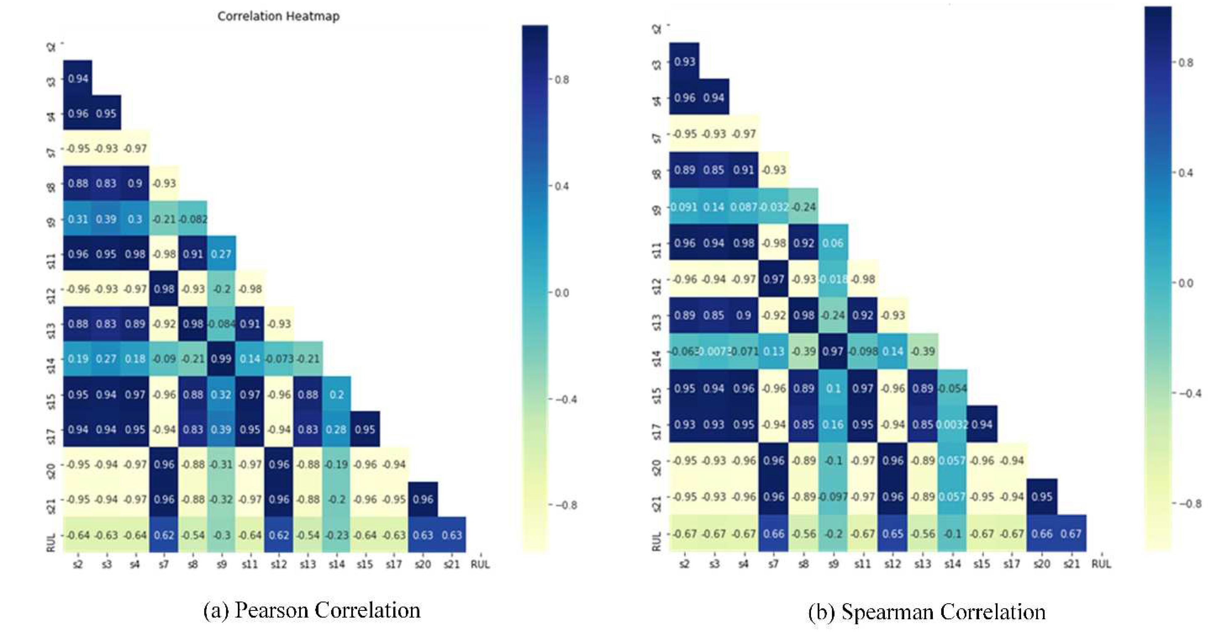
4.1. Introduction of the Aero-Engine Dataset and Preprocessing

In this experiment, the NASA Aeroengine CMAPSS dataset [34] is selected to verify the proposed algorithm. The CMAPSS software simulates the operation of the engine system, the fault and performance degradation process of the main rotating parts, and outputs the performance parameters with noise. Because of its high fidelity and high data quality, it is widely used in the field of RUL prediction.

The aero-engine monitoring data includes temperature, pressure, speed, etc., with a total of 26 parameters. The first parameter represents the ID of the aero-engine. The second represents the number of flight cycles. The third to fifth parameters are working condition parameters, and other fields are the running status parameters.

Table 1. Key components of the aero-engine and the monitoring parameters characterized the failure.

	Part Name	Monitoring Parameters Characterize Failure
1	Aero-engine blade	Fan speed, fan inlet pressure, temperature, etc.
2	Aero-engine main bearing	Rotor speed, gas path pressure, turbine flow, etc.
3	Connecting bolt of the aero-engine rotor	Rotor speed, gas path pressure, temperature, etc.

summarizes the monitoring parameters that can characterize the failure of the key components of an aero-engine. This dataset includes the temperature, pressure, flow and other parameters of an aero-engine, thus, reflecting the degradation state of an engine.

Table 2. Variance of normalized parameters.

Parameters	Variance	Parameters	Variance
s1	0.005532	s12	0.157257
s2	0.150615	s13	0.105761
s3	0.133660	s14	0.098440
s4	0.151931	s15	0.144302
s5	0.005215	s16	0.007783
s6	0.010709	s17	0.129060
s7	0.142523	s18	0.005741
s8	0.107551	s19	0.006879
s9	0.099086	s20	0.140110
s10	0.015037	s21	0.149473
s11	0.158977

shows the variance of each field of normalized data. The variance of s1, s5, s6, s10, s16, s18 and s19 is less than 0.02, which is significantly less than the variance of other fields and can be eliminated. To investigate the correlations between different features, Pearson correlation analysis and Spearman correlation analysis can be used [35]. As shown in Figure 8, the correlation heatmap shows that the Pearson coefficient and Spearman coefficient of S9, S14 and RUL are significantly smaller than those of other features, thus, representing that the correlation between S9 and S14 and RUL is the smallest. At last, the features including s1, s5, s6, s9, s10, s14, s16, s18 and s19 are removed from the original data.

4.2. Experiment Results and Analysis

4.2.1. HI Construction Results and Analysis

According to the analysis of the original data, the data after feature selection are fused through PCA dimension reduction. For dimension reductions, different dimension reduction methods including PCA and Locality Preserving Projections are tried in the experiment. Additionally, the two-dimensional data obtained through PCA are easy to observe and have the best prediction effect. The center of health stage, rapid degradation stage and near-failure stage are $(-4.29\times {10}^{-1}, 4.24\times {10}^{-4})$, $(5.04\times {10}^{-2},-1.13\times {10}^{-3})$ and $(6.90\times {10}^{-1}, 2.28\times {10}^{-3})$ respectively found through FCM clustering. The clustering results of historical data are shown in Figure 9a. Taking the engine 1 as an example, the membership degree change curve of each degradation stage is shown in Figure 9b.

The figure shows that the degradation process is well divided by fuzzy clustering, and the three membership degree curves represent the membership degree of different stages, thus, indicating that the method proposed in this paper can identify the degradation stage well.

As the degradation process and failure mechanism of engines are different, the degradation benchmark and failure benchmark are not suitable as the measurement benchmark. In this paper, the health benchmark is selected as the measurement benchmark. The distance to health base curve of historical data is shown in Figure 10a. With the increase in cycle times, the engine gradually deviates from the healthy state. In order to facilitate the follow-up study, the health-base distance is converted into HI, as shown in Figure 10b. The constructed health factor improves the problem of using the membership degree as the HI, and meets the three requirements of the monotonicity, robustness and divisibility of HI.

The prediction is made according to the relevant parameters learned by the fuzzy clustering. The prediction results are shown in Figure 11a. The data distribution is consistent with the historical data. Similarly, the health factors to be predicted are constructed, and the relevant degradation trajectories are obtained, as shown in Figure 11b.

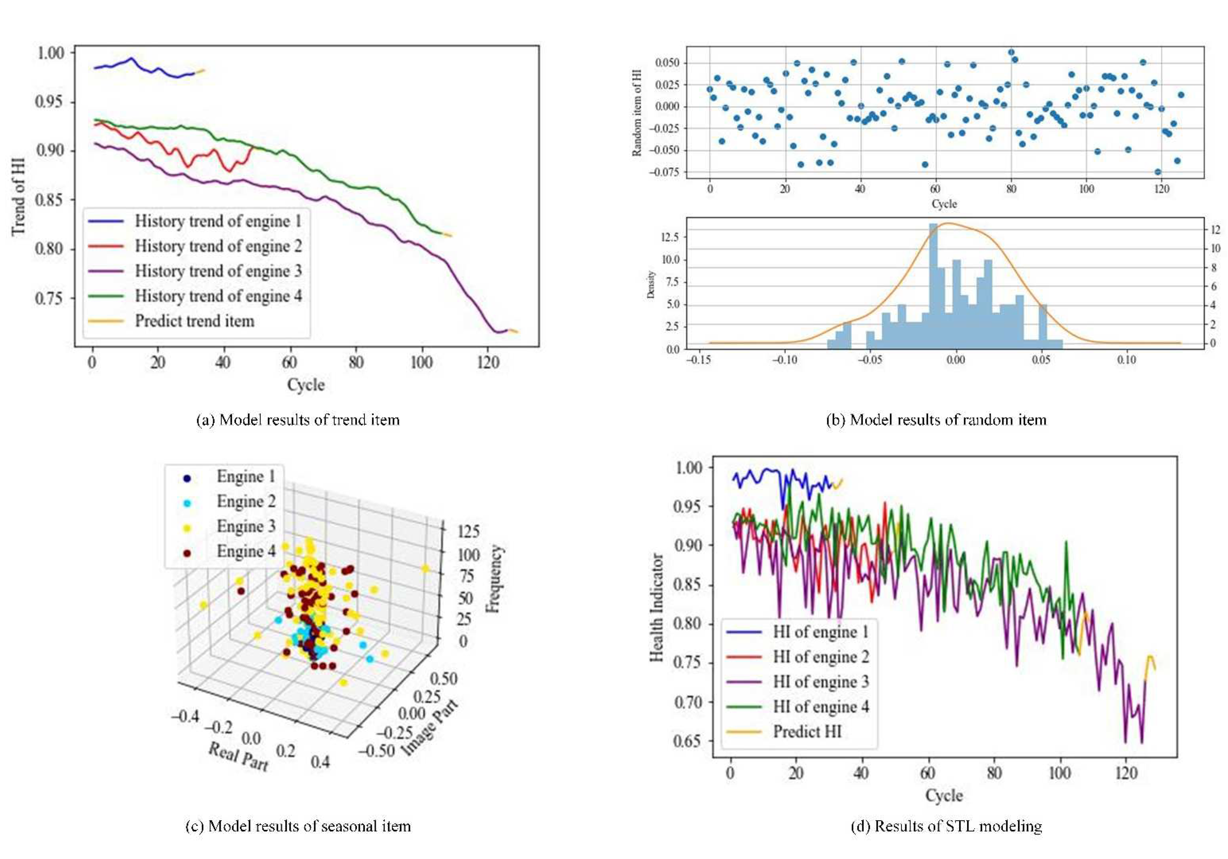
4.2.2. STL Modeling Results and Analysis

In order to solve the problem of poor predictions based on historical data, the time-series decomposition modeling and predictions are introduced. First, the STL decomposition is implemented on the data to be predicted. Taking engines 3 and 4, for example, the decomposition results of the trend term, seasonal term and random term are shown in Figure 12. The influence of the random term is removed from the trend term after decomposition, which is convenient for modeling and predictions. Each engine’s seasonal term and random term are different, so independent modeling is also required.

Taking engines 1, 2, 3 and 4, for example, ARIMA is used to model the trend term of each engine. The model parameters and evaluation results are shown in

Table 3. ARIMA models.

Engine ID	Model	Log Likelihood	AIC	BIC	HQIC
1	SARIMAX(0, 2, 0)	143.074	−284.149	−282.781	−283.721
2	SARIMAX(0, 1, 1)	216.029	−428.057	−424.315	−426.643
3	SARIMAX(1, 1, 1)	673.926	−1339.852	−1328.539	−1335.256
4	SARIMAX(0, 1, 3)	564.176	−1118.351	−1105.081	−1112.974

, and the prediction results of the trend term are shown in Figure 13a.

For the random term, KDE is used to estimate the random-term’s distribution. Taking engine 3, for example, the random term distribution, histogram and KDE curve is shown in Figure 13b. For each engine, the random term is modeled by this method, and then the predicted random term is generated by acceptance–rejection sampling. For the seasonal term, taking engines 1, 2, 3 and 4, for example, the amplitude and phase angle of each frequency are obtained by FFT. As shown in Figure 13c, the imaginary number represents the amplitude and phase angle of each frequency for each engine. The modeling of the seasonal term is completed by selecting several frequencies with large modulus values. The synthesis results of the final three models are shown in Figure 13d. It can be found that the multi-step prediction results conform to the degradation trend and have a good imitation of the periodicity and randomness of degradation.

4.2.3. RUL Prediction Results and Analysis

The HI degradation trajectory constructed by fuzzy clustering and predicted by STL decomposition modeling have noise. The sliding average filtering is used to smooth them to facilitate the subsequent similarity measurement and improve the accuracy of the RUL prediction. As shown in Figure 14, the degradation tracks after filtering are smooth and have obvious characteristics, which is convenient for similarity comparisons.

There are usually two kinds of evaluation indexes for the RUL prediction of an aero-engine: mean square error (MSE) and score. MSE is applicable to all kinds of prediction problems, and the score is the RUL prediction evaluation index proposed by the data publisher. In addition, the true RUL is obtained from the NASA repository. The calculation formula is as follows:

$$MSE=\frac{1}{N}{\displaystyle \sum _{t=1}^N{(r_t{}^{ture}-r_t{}^{predict})}^2}$$

(27)

$$s=\left\{\begin{array}{c}{\displaystyle \sum _{i=1}^n}{e}^{-\left(\frac{d}{a_1}\right)}-1, d<0\\ {\displaystyle \sum _{i=1}^p}{e}^{\left(\frac{d}{a_2}\right)}-1, d>0\end{array}\right.$$

(28)

where $d=r^{ture}-r^{predict}$, $a_1=13, a_2=10$.

The method proposed is tested on the dataset, and the prediction results are shown in

Table 4. RUL prediction results.

	MSE	Score
Prediction without the STL model	570	1401
Prediction with the STL model	528	1280
Improved degree	8.0%	9.5%

. In the two indicators, the proposed model is better than the model without degradation decomposition. The specific prediction results of each engine are shown in Figure 15. In fact, only a few engines’ prediction results have a certain deviation, and most of the predictions are consistent with true RUL. The RUL has bias towards safe prediction.

The change curves of MSE of the two methods under the different numbers of most similar trajectories are shown in Figure 16. The RUL prediction method with STL decomposition modeling performed better generally. The effectiveness of the proposed algorithm is illustrated.

To illustrate the effectiveness and accuracy of the proposed method, the support vector machine (SVM), ARIMA-SVM, multilayer neural network (MLP), long short-term neural network (LSTM) and other algorithms are selected for the comparative test. The proposed method is denoted as FCM-STL-TSBP. The detailed results are shown in

Table 5. Comparison test results.

Method	MSE	Score
SVM [36]	1658	N/A
ARIMA-SVM [37]	1575	N/A
MLP [38]	1411	N/A
LSTM [39]	541	1116
FCM-TSBP	570	1401
FCM-STL-TSBP	528	1280

.

The prediction results of deep learning, such as LSTM, are better than shallow learning results, such as SVM and MLP. The proposed method performs better on MSE, and the score is close to LSTM. Additionally, the proposed method has great advantages. And the history HI database can update dynamically with the increase in flight data and the model can learn online. The MSE improved 8.0% and the score improved 9.5% compared to FCM-TSBP.

5. Conclusions

This paper presents a method to predict the RUL for an aero-engine based on time-series degradation modeling and similarity comparisons. This paper mainly considers the following three issues: the construction of HI of multi-dimensional monitoring data, the accurate modeling of the single engine degradation trajectory and the similarity comparison method of the degradation trajectory. The first problem is solved by fuzzy clustering and HI transformation. The second problem is solved by STL decomposition, and each item is modeled respectively. And the third problem is solved by similar segment positioning and dynamic weight predictions. In particular, the introduction of the predictive degradation trajectory improves the original prediction accuracy. Finally, the effectiveness of the proposed method is verified by experiments on the dataset from NASA.

References

1. Nie, L.; Xu, S.; Zhang, L.; Yin, Y.; Dong, Z.; Zhou, X. Remaining Useful Life Prediction of Aeroengines Based on Multi-Head Attention Mechanism. Machines 2022, 10, 552. [Google Scholar] [CrossRef]
2. Lei, Y.; Li, N.; Gontarz, S.; Lin, J.; Radkowski, S.; Dybala, J. A model-based method for remaining useful life prediction of machinery. IEEE Trans. Reliab. 2016, 65, 1314–1326. [Google Scholar] [CrossRef]
3. El-Tawil, K.; Jaoude, A.A. Stochastic and nonlinear-based prognostic model. Syst. Sci. Control Eng. Open Access J. 2013, 1, 66–81. [Google Scholar] [CrossRef] [Green Version]
4. Paroissin, C. Inference for the Wiener process with random initiation time. IEEE Trans. Reliab. 2015, 65, 147–157. [Google Scholar] [CrossRef]
5. Wang, B.; Lei, Y.; Li, N.; Li, N. A hybrid prognostics approach for estimating remaining useful life of rolling element bearings. IEEE Transac. Reliabil. 2018, 69, 401–412. [Google Scholar] [CrossRef]
6. Li, H. Statistical Learning Methods; Tsinghua University Press: Beijing, China, 2012; pp. 1–2. [Google Scholar]
7. Zhang, B.; Zheng, K.; Huang, Q.; Feng, S.; Zhou, S.; Zhang, Y. Aircraft engine prognostics based on informative sensor selection and adaptive degradation modeling with functional principal component analysis. Sensors 2020, 20, 920. [Google Scholar] [CrossRef] [Green Version]
8. Zaidan, M.A.; Mills, A.R.; Harrison, R.F.; Fleming, P.J. Gas turbine engine prognostics using Bayesian hierarchical models: A variational approach. Mech. Syst. Signal Process. 2016, 70, 120–140. [Google Scholar] [CrossRef]
9. Liu, K.; Huang, S. Integration of data fusion methodology and degradation modeling process to improve prognostics. IEEE Trans. Autom. Sci. Eng. 2014, 13, 344–354. [Google Scholar] [CrossRef]
10. Song, C.; Liu, K. Statistical degradation modeling and prognostics of multiple sensor signals via data fusion: A composite health index approach. IISE Trans. 2018, 50, 853–867. [Google Scholar] [CrossRef]
11. Cui, L.-F.; Zhang, Q.-Z.; Shi, Y.; Yang, L.-M.; Wang, J.-L.; Bai, C.-G. A method for satellite time series anomaly detection based on fast-DTW and improved-KNN. Chin. J. Aeronaut. 2022, in press. [Google Scholar] [CrossRef]
12. Kim, M.; Song, C.; Liu, K. A generic health index approach for multisensor degradation modeling and sensor selection. IEEE Trans. Autom. Sci. Eng. 2019, 16, 1426–1437. [Google Scholar] [CrossRef]
13. Zhang, J.; Dong, Z.; Shi, H. Real-time remaining useful life prediction based on adaptive kernel window width density. Meas. Sci. Technol. 2022, 33, 105122. [Google Scholar] [CrossRef]
14. Deutsch, J.; He, D. Using deep learning-based approach to predict remaining useful life of rotating components. IEEE Trans. Syst. Man Cybern. Syst. 2017, 48, 11–20. [Google Scholar] [CrossRef]
15. Deutsch, J.; He, M.; He, D. Remaining useful life prediction of hybrid ceramic bearings using an integrated deep learning and particle filter approach. Appl. Sci. 2017, 7, 649. [Google Scholar] [CrossRef] [Green Version]
16. Zhao, G.; Zhang, G.; Liu, Y.; Zhang, B.; Hu, C. Lithium-ion battery remaining useful life prediction with deep belief network and relevance vector machine. In Proceedings of the 2017 IEEE International Conference on Prognostics and Health Management (ICPHM), IEEE, Dallas, TX, USA, 19–21 June 2017; pp. 7–13. [Google Scholar]
17. Liu, R.; Yang, B.; Hauptmann, A.G. Simultaneous bearing fault recognition and remaining useful life prediction using joint-loss convolutional neural network. IEEE Trans. Ind. Inform. 2019, 16, 87–96. [Google Scholar] [CrossRef]
18. Jiao, R.; Peng, K.; Dong, J. Remaining useful life prediction for a roller in a hot strip mill based on deep recurrent neural networks. IEEE/CAA J. Autom. Sin. 2021, 8, 1345–1354. [Google Scholar] [CrossRef]
19. Fu, B.; Yuan, W.; Cui, X.; Yu, T.; Zhao, X.; Li, C. Correlation analysis and augmentation of samples for a bidirectional gate recurrent unit network for the remaining useful life prediction of bearings. IEEE Sens. J. 2020, 21, 7989–8001. [Google Scholar] [CrossRef]
20. Cui, L.-F.; Zhang, Q.-Z.; Yang, L.-M.; Bai, C.-G. A Performance Prediction Method Based on Sliding Window Grey Neural Network for Inertial Platform. Remote Sens. 2021, 12, 4864. [Google Scholar] [CrossRef]
21. Han, X.-X.; Xiang, G.; Cui, L.-F.; Wang, J.-L.; Zhang, Q.-Z.; Lin, R.-S.; Jin, Y.; Liu, H.-D. Online Transfer Learning-based Method for Predicting Remaining Useful Life of Aero-engines. In Proceedings of the 2022 7th International Conference on Intelligent Computing and Signal Processing, Virtual, 15–17 April 2022. [Google Scholar]
22. Wang, B.; Lei, Y.; Yan, T.; Li, N.; Guo, L. Recurrent convolutional neural network: A new framework for remaining useful life prediction of machinery. Neurocomputing 2020, 379, 117–129. [Google Scholar] [CrossRef]
23. Liu, J.; Li, Q.; Chen, W.; Yan, Y.; Qiu, Y.; Cao, T. Remaining useful life prediction of PEMFC based on long short-term memory recurrent neural networks. Int. J. Hydrogen Energy 2019, 44, 5470–5480. [Google Scholar] [CrossRef]
24. Xiao, L.; Zhang, L.; Niu, F.; Su, X.; Song, W. Remaining Useful Life Prediction of Wind Turbine Generator Based on 1D-CNN and Bi-LSTM. Int. J. Fatigue 2022, 163, 107051. [Google Scholar] [CrossRef]
25. Li, C.; Zhang, H.; Wang, C.; Li, X.; Lu, Y.; Qian, C. An Efficient Yinyang k-Means Clustering Algorithm. J. Jilin Univ. Sci. Ed. 2021, 59, 1455–1460. [Google Scholar]
26. Wu, C.; Qi, S. Adaptive weighted K-nearest neighbor fingerprint location algorithm based on improved K-means clustering. J. Chongqing Univ. Posts Telecommun. (Nat. Sci. Ed.) 2021, 33, 946–954. [Google Scholar]
27. Liu, Y.; Zhang, Y.; Zheng, W. Optimization research of denoised hierarchical mapping analysis for multidimensional cluster analysis. J. Sichuan Univ. (Nat. Sci. Ed.) 2022, 59, 84–92. [Google Scholar]
28. Saxena, A.; Prasad, M.; Gupta, A.; Bharill, N.; Patel, O.P.; Tiwari, A.; Er, M.J.; Ding, W.; Lin, C.T. A review of clustering techniques and developments. Neurocomputing 2017, 267, 664–681. [Google Scholar] [CrossRef] [Green Version]
29. Ruspini, E.H.; Bezdek, J.C.; Keller, J.M. Fuzzy clustering: A historical perspective. IEEE Comput. Intell. Mag. 2019, 14, 45–55. [Google Scholar] [CrossRef]
30. Pu, X.; Huang, J.; Qi, N.; Song, C. Application of K-Means Algorithm Based on Density Information Entropy in Customer Segmentation. J. Jilin Univ. Sci. Ed. 2021, 59, 1245–1251. [Google Scholar]
31. Wang, H.; Cui, W.; Xu, P.; Li, C. Optimization of Canopy on K Selection in Partition Clustering Algorithm. J. Jilin Univ. (Sci. Ed.) 2020, 58, 634–638. [Google Scholar]
32. Cleveland, R.B.; Cleveland, W.S.; Terpenning, I. STL: A Seasonal-Trend Decomposition Procedure Based on Loess. J. Off. Stat. 1990, 6, 3–73. [Google Scholar]
33. Zhang, Q.-Z.; Zhang, Q.-Q.; Cui, L.-F.; Han, X.-X.; Jin, Y.; Xiang, G.; Shi, Y. A method for measuring similarity of time series based on series decomposition and dynamic time warping. Appl. Intell. 2022, 6. [Google Scholar] [CrossRef]
34. Saxena, A.; Goebel, K.; Simon, D.; Eklund, N. Damage propagation modeling for aircraft engine run-to-failure simulation. In Proceedings of the 2008 International Conference on Prognostics and Health Management, IEEE, Denver, CO, USA, 6–9 October 2008; pp. 1–9. [Google Scholar]
35. Cui, L.-F.; Wang, L.; Xiang, G.; Zhang, Q.-Z.; Bai, C.-G.; Yang, G.-B. A Method Based on Correlation Analysis of the Assembly Process and Neural Network for Precision Prediction of the Inertial Platform. In Proceedings of the ICCBDC 2021–2021 5th International Conference on Cloud and Big Data Computing, New York, NY, USA, 20–22 August 2021. [Google Scholar]
36. Zhang, C.; Lim, P.; Qin, A.K.; Tan, K.C. Multiobjective deep belief networks ensemble for remaining useful life estimation in prognostics. IEEE Trans. Neural Netw. Learn. Syst. 2016, 28, 2306–2318. [Google Scholar] [CrossRef] [PubMed]
37. Yan, H.; Zuo, H.; Sun, J.; Zhou, D.; Wang, H. Two-Stage Degradation Assessment and Prediction Method for Aircraft Engine Based on Data Fusion. Int. J. Aerosp. Eng. 2021, 1–16. [Google Scholar] [CrossRef]
38. Miao, H.; Li, B.; Sun, C.; Liu, J. Joint learning of degradation assessment and RUL prediction for aeroengines via dual-task deep LSTM networks. IEEE Trans. Ind. Inform. 2019, 15, 5023–5032. [Google Scholar] [CrossRef]
39. Li, H.; Li, Y.; Wang, Z.; Li, Z. Remaining Useful Life Prediction of Aero-Engine Based on PCA-LSTM. In Proceedings of the 2021 7th International Conference on Condition Monitoring of Machinery in Non-Stationary Operations (CMMNO), IEEE, Guangzhou, China, 11–13 June 2021; pp. 63–66. [Google Scholar]
Figure 1. Aero-engine.
Aerospace 09 00609 g001
Figure 2. The overall framework for RUL predictions based on STL modeling and similarity measurements.
Aerospace 09 00609 g002
Figure 3. Degradation stages of an aero-engine.
Aerospace 09 00609 g003
Figure 4. HI construction based on fuzzy clustering.
Aerospace 09 00609 g004
Figure 5. Degradation path prediction based on STL modeling.
Aerospace 09 00609 g005
Figure 6. RUL prediction based on similarity comparison.
Aerospace 09 00609 g006
Figure 7. Segment similarity comparison.
Aerospace 09 00609 g007
Figure 8. Correlation coefficient analysis.
Aerospace 09 00609 g008
Figure 9. Fuzzy cluster result and membership degree curve.
Aerospace 09 00609 g009
Figure 10. Distance to health base and health indicator.
Aerospace 09 00609 g010
Figure 11. FCM predict results and predicted HI paths.
Aerospace 09 00609 g011
Figure 12. Degradation trajectory decomposition.
Aerospace 09 00609 g012
Figure 13. STL decomposition modeling result.
Aerospace 09 00609 g013
Figure 14. HI degradation trajectory.
Aerospace 09 00609 g014
Figure 15. RUL prediction results of each engine.
Aerospace 09 00609 g015
Figure 16. MSE curve with the number of most similar trajectories.
Aerospace 09 00609 g016