Article

Experimental Investigation of a Roughness Element Wake on a Hypersonic Flat Plate

College of Aerospace Science and Engineering, National University of Defense Technology, Changsha 410073, China
*
Author to whom correspondence should be addressed.
Aerospace 2022, 9(10), 574; https://doi.org/10.3390/aerospace9100574
Submission received: 31 August 2022 / Revised: 19 September 2022 / Accepted: 25 September 2022 / Published: 2 October 2022

Abstract

:
An experimental investigation was performed on the wake flow field of an isolated roughness element of a flat plate at Mach 6 by employing the nanoparticle-based planar laser scattering (NPLS) approach. The three-dimensional features and causes of the flow field structure were scrutinized by transient flow field images of roughness elements on various planes. The time-resolved NPLS technique was implemented to examine the time evolution characteristics of the wake flow field of roughness elements. In the following, the process of dynamic evolution of large-scale vortex structures in the wake flow field was methodically assessed. Additionally, the influences of roughness element heights on the wake vortex structure were evaluated and the obtained results were compared.

1. Introduction

Hypersonic boundary layer transitions from laminar to turbulent causes skin friction and heat flux in hypersonic vehicle surfaces to increase by an order of magnitude [1]. Therefore, the laminar–turbulent transition in the hypersonic boundary layer represents a crucial factor in the design of hypersonic vehicles [2], particularly for thermal protection systems and aerodynamic design [3]. In real flight environments, the thermal protection system on the surface of hypersonic vehicles will form irregular protrusions or pits due to a physical collision or high-temperature ablation [4,5]. On the other hand, in order to enhance the starting performance of the aircraft inlet, a forced-transition trip is often installed in the inlet to lessen the flow separation [6]. In engineering applications, the protrusions or pits on the surface of these aircrafts and the installed forced-transition trip can be regarded as small roughness elements. The existence of these roughness elements will affect the process of boundary layer transition, thereby affecting the aerodynamic performance of the aircraft [7]. The understanding of the mechanisms of hypersonic boundary layer transition is still not sufficient, but wind tunnel experiments are an important research method [8]. Therefore, the experimental investigation on the hypersonic wake flow field of roughness elements is helpful to realize the influence of roughness elements on the characteristics of the boundary layer transition. Further, such assessments and explorations provide a solid basis for the accurate prediction and effective control of the boundary layer transition.
There are many factors impacting the wake flow field of supersonic/hypersonic roughness elements, including the type of the roughness element (isolated or distributed), geometric parameters (height [9], width, shape, and spacing between nearby roughness elements [10]), and aerodynamic parameters (boundary layer thickness, Reynolds number, Mach number [11], wall temperature [4], and freestream noise [12]). Compared to the distributed roughness element, the isolated roughness element is the most common type of roughness element and is also the basis of roughness element research. In recent decades, a lot of explorations have been performed to address the influence of isolated roughness elements on the characteristics of the wake flow field. It is well known that the roughness element height (REH) becomes one of the main factors influencing the wake flow field as the aspect ratio of the roughness element is fixed. Van Driest and McCauley [9] aimed to explore the influence of the height of spherical roughness elements on the boundary layer transition at supersonic. The obtained results revealed that within a specific height range, the roughness element would trigger the boundary layer transition in advance, and the REH corresponding to the transition position closest to the upstream roughness element was defined as the effective REH. In order to make the data of REH reasonable and meaningful, Van Driest and Blumer [13] scrutinized the relationship between the effective REH k e f f and the boundary layer displacement thickness δ x k * at the roughness element position x k . Braslow et al. [14] utilized the roughness element Reynolds number R e k in terms of the REH by R e k = k U k / ν , where U k denotes the unperturbed velocity, k represents the REH, and υ stands for the kinematic viscosity. Sydney and Kitchens [15] classified the size of isolated roughness elements in supersonic flow by the ratio of the REH to the local boundary layer thickness ( k / δ k ). It was noticed that in the case of k δ k , it would be categorized as a small roughness element, and the influence of roughness elements on the boundary layer would be much smaller. Schneider [16] emphasized that one of the leading purposes of analyzing the effect of roughness elements on the boundary layer transition under hypersonic conditions is to determine the critical REH that begins to affect the boundary layer transition. Chuvakhov [17] verified the typical law of the effect of REH on the boundary layer transition and distinguished three different regimes depending on k / δ k . For the small value of k / δ k , the wake flow attenuates rapidly and does not affect the transition station. Increasing k / δ k to the critical value, the wake flow breaks down into a turbulent wedge with the apex ahead of the natural transition station. As k / δ k reaches the effective value, the transition position no longer changes, and the increase in k / δ k cannot promote the transition position but disturbs the flow more.
In order to determine both the critical and effective REHs and examine the impact of the isolated roughness element on the wake flow field, it is necessary to acquire the space–time structure of the wake flow field and compare the influence of various REHs on the space–time structure. Wheaton and Schneider [18,19] obtained the fluctuating component of pressure to locate evidence of instabilities within the roughness element wake via wall-mounted pressure transducers along the wake centerline. The surface pressure measurement yielded to the identification of several dominant disturbance frequencies in the transition process, but only at specific locations. As a powerful methodology for inspecting the flow field structure, the flow visualization approach has been broadly implemented to examine the wake flow field of supersonic/hypersonic roughness elements. Whitehead [10] exploited the oil flow technology to investigate the typical flow field of roughness elements on a wedge surface at Mach 6.8, and the bow shock wave and reverse rotating vortexes were detected. Skuratov and Fedorov [20] measured the distribution of the heat transfer coefficient of roughness element wake on the surface of the 5° sharp cone at Mach 6 by using thermal indicator coatings. The obtained results proved that the boundary layer transition relies on the Reynolds number of the incoming flow and the REH. Kuester and White [21] assessed the structure of the turbulent wedge downstream of the roughness element by Naphthalene shear stress visualization and hotwire measurements. The experimentally observed data demonstrate that the expansion of the turbulent wedge is related to the high- and low-speed streaks. Flow visualization methods such as oil flow and temperature sensitive paint can well display the wall flow; however, they cannot reflect the spatial and transient structure of the wake flow. In order to obtain the spatial flow structure above the wall, Lash et al. [22] examined the shock wave–boundary layer interactions in a transitional boundary layer by employing time-resolved Schlieren visualization. An image processing script could be exploited to track the positions of shock structures to characterize the dynamic shock behavior. Compared with the wall measurements, the Schlieren visualization was capable of capturing the shock wave, but the flow structure was still challenging to identify inside the boundary layer.
For visualizing the flow field inside the boundary layer, laser diagnosis technology can obtain the three-dimension transient flow structure of the supersonic/hypersonic flow field, which is extensively employed in the study of roughness element wake flow field. Murphree et al. [23] utilized planar laser scattering and particle image velocimetry to visualize the upstream flow structure of the roughness element on the Mach 5 plate. The flow structure and instability characteristics of the shock wave–boundary layer interaction produced by the roughness element in natural transition and full turbulence were then compared. The results indicated that the separated flow region of transitional interactions exhibits larger variations in their scale and shape than fully turbulent interactions. Wang et al. [24] carried out an experimental investigation of supersonic flow over a hemisphere using nanoparticle-based planar laser scattering (NPLS) technique in a supersonic quiet wind tunnel at Mach 2.68. The evolution process of the large-scale vortex structure with the features of periodicity and similar geometry was observed and reported. In order to further examine the evolution process of the roughness element wake flow, Jiang et al. [25] employed the nitric-oxide planar laser-induced fluorescence technique to gain the time-dependent image sequence of 160 pixel × 160 pixel with a time resolution of 500 kHz. The time evolution process of the corkscrew-shaped vortex in the Mach 10 roughness element wake field was also given, and streak instability was identified. In order to scrutinize the influence of different REHs on the flow field structure, combined with NPLS and WCNS-E-5 numerical schemes, Zhao and Gang et al. [26,27] performed a flow visualization and a numerical simulation of the wake flow field of a rough element with various heights on Mach 3 plate. The results showed that for the small levels of the REH, the shear layer instability in the wake region dominated the boundary layer transition. Nevertheless, for the larger height roughness element, the instability in the upstream separation region becomes the dominant mechanism of the boundary layer transition. He et al. [28] visualized the shock–shock interference induced by a cylindrical protuberance mounted perpendicular to a hollow cylinder at Mach 2.95, and the fine interference structures were captured and analyzed in detail.
A large number of experimental studies on the wake flow field of supersonic roughness elements have been carried out by the flow visualization approach, and many significant results have been reported. However, flow visualization on the wall surface cannot reflect the spatial structure of the boundary layer, and most of the research on the spatial structure of the boundary layer has been focused on the flow display of a single plane structure, which cannot fully reveal the three-dimensional characteristics of the flow field structure. Additionally, there are relatively few investigations on the time evolution characteristics of the wake flow field of the hypersonic roughness element. On the other hand, the images may be not clear enough since it is difficult to methodically take into account the spatial resolution of the image when it reaches a high time resolution (microsecond level). In the current paper, the wake flow field of isolated roughness elements on a Mach 6 plate is explored experimentally by using a self-developed time-resolved NPLS system. The system can continuously shoot eight high-resolution image sequences at the repetition rate of 1 MHz. Through the fine structure of the wake flow field of various plane roughness elements, the three-dimensional features of the flow structure are scrutinized. The time evolution characteristics of the wake flow field of the roughness element are examined by the time-resolved flow field structure with a 200 kHz time resolution, and then the variation rules of the wake flow field structure under the influence of different REHs are compared.

2. Experimental Equipment

2.1. Hypersonic Low Noise Wind Tunnel

The experiments were carried out in the hypersonic low-noise wind tunnel in the Aerodynamics Laboratory at the National University of Defense Technology. The schematic representation of the wind tunnel structure is demonstrated in Figure 1. The wind tunnel adopts a straight-through design and blowdown-indraft operation. The single effective operation time of the wind tunnel is higher than 15 s. The high-temperature and high-pressure flow is appropriately dried and filtered. In order to restrain the freestream noise, rectification fits such as a wide-angle diffuser, acoustic baffles, and damping net are installed in the settling chamber. The length of the test chamber is 800 mm, and the cross-section dimensions are 260 mm × 260 mm. Large-size optical observation windows are installed on four sides, providing convenience for flow field observations in multiple directions.
This experiment was performed at a Mach number of 6, the total temperature and nominal total pressure were set equal to 350 K and 0.85 MPa, respectively. There was a slight variation between the actual pressure and set pressure during the operation (with a relative error of less than 6%). The freestream pressure fluctuation level was lower than 0.5%, which was qualified by the high-frequency pressure transducer (Kulite XCE-62 by Kulite Semiconductor Products, Inc. from Leonia, State of New Jersey, USA). The detailed wind tunnel operation parameters are given in Table 1.

2.2. Test Model

As shown in Figure 2, the streamwise length, spanwise width, and thickness of the metal smooth flat plate were 600 mm, 250 mm, and 20 mm, respectively. The bluntness of the plate leading edge was less than 0.1 mm. The plate was installed in the test chamber at a distance of 100 mm from the bottom of the test section, the leading edge was placed in the nozzle exit section, and the attack angle of the plate was set as 0°. The boundary layer to be measured developed on the plate with a zero nominal pressure gradient. The test measurement area was marked with a red rectangle.
The space rectangular coordinate system was established in this research as follows, and the coordinate origin was located in the center of the leading edge of the plate. The x-axis and y-axis were associated with the flow direction and upward direction perpendicular to the plate, respectively, and the z-axis was determined based on the right-hand coordinate system (see Figure 3). The xy-plane, yz-plane, and xz-plane in order were defined as the streamwise plane, normal plane, and spanwise plane. The cylindrical isolated roughness element with diameter d = 6 mm was installed at 133.3 mm in the x-axis direction, and its height k could be adjusted in the range of 1–5 mm.

2.3. Time-Resolved NPLS System

The time-resolved NPLS system was utilized to investigate the dynamic evolution of the flow structure, and the schematic representation of the NPLS system is presented in Figure 4. The system mainly includes a nanoparticles generator, eight-pulse Nd:YAG laser, synchronous controller, imaging system, and computer data acquisition system. The nanoparticles were uniformly scattered upstream by the nanoparticle generator, and the eight-pulse Nd:YAG laser produced the laser slice illumination flow field with a MHz-repetition-rate. The imaging system consisted of eight-CCD cameras placed side by side, and the CCD camera output a 16-bit gray image with a resolution of 1952 pixel × 1112 pixel. Each pulse laser worked synchronously with a single CCD camera through the synchronous controller. TiO2 nanoparticles with a diameter of 50 nm were implemented as tracers, the laser pulse wavelength, width, and energy in order were 532 nm, 6 ns, and 300 mJ/pulse. The thickness of the beam waist was also about 0.5 mm. In this experiment, a series of images were acquired with a 200 kHz time resolution.
The eight cameras were placed side by side, and each CCD camera was not parallel to the sheet light plane, making it impossible to achieve a clear focus image of the entire test area (see Figure 5a). To solve this problem, the tilt-shift (TS) mechanism was applied for auxiliary focus, with the corresponding technical details as displayed by Sun et al. [29]. The same checkerboard images taken without/with the TS mechanism are presented in Figure 5a,b. The right side of the chessboard image was blurred without the TS mechanism, and the image became clearer after using the TS mechanism.
Due to the different positions of the CCD camera and the use of the TS mechanism, the field of view of each camera had a slight difference and deformation. In order to study the time evolution characteristics of the flow structure, each camera imaging area should be consistent. The image calibration method by Zhang [30] was implemented to calibrate each camera image based on the plane checkerboard. Figure 6 presents the pixel error distribution of the corners by cameras 2–8 relative to the corresponding corners by camera 1 after calibration. The maximum pixel error was less than 0.34 pixel and the average pixel error was only 0.07 pixel, which verified the accuracy of the image calibration method utilized in this paper.

3. Results and Discussion

3.1. Boundary Layer Transient Flow Structure of the Smooth Plate in the xy-Plane

In order to compare the influence of the roughness element on the wake flow field, the flow structure without the roughness element was firstly analyzed and taken as the reference flow field. The transient flow field image of the boundary layer of a smooth flat plate in the xy-plane is displayed in Figure 7. The range of the flow field was specified by x = 110 mm–310 mm, y = 0 mm–15 mm, and the spatial resolution of the image was 103 μm/pixel. The flow direction was considered from left to right and the actual unit Reynolds number was 1.29 × 10⁷ m−1.
Since the thickness of the hypersonic laminar boundary layer was thin and the velocity gradient was large, it was difficult to perform accurate velocity distribution measurements to evaluate the boundary layer thickness. Therefore, the boundary layer thickness was determined based on the image structure. The tracer particles were uniformly scattered in the supersonic flow field. Due to the good following property of nanoparticles, in the region of the low-density flow field, the particle concentration was low, and the corresponding image brightness was low, as described by Tian et al. [31]. As we know, the flow field density inside the boundary layer is lower than that of the external mainstream flow field. Therefore, in Figure 7, the dark area at y = 0–2 mm is pertinent to the interior of the boundary layer, and the relatively light area at y = 2–15 mm is associated with the mainstream. In the present paper, the height of the dark area was exploited to define the boundary layer thickness. Actually, in the laminar boundary layer, due to the Magnus effect [32] and the leading-edge lift effect [33], some of the particles were thrown out of the boundary layer and eventually moved along the streamline. Other ones moved toward the wall due to the influence of the Suffman lift force [33], leading to the light–dark step change in the boundary layer region of the NPLS image. This implies that there was a specific error between the boundary layer thickness based on the image structure and the real one. Furthermore, the former may increase with the growth of the real boundary layer thickness. Huntley [34] found the same phenomenon by applying the filtered Rayleigh scattering technology to analyze the boundary layer transition on a Mach 8 elliptic cone, indicating that the boundary layer thickness based on the image structure was about 10% thinner than the real one. Therefore, the thickness of the dark area in Figure 7 can qualitatively represent the boundary layer thickness, and it was thinner than the real one. The plotted results in Figure 7 show that the flow field remained laminar and there was no instability in the boundary layer. The roughness elements were planned to be installed in the red rectangular region. According to the image approach, the boundary layer thickness δ was approximately obtained as 2 mm, and this value was utilized as the reference for evaluating the dimensionless factor of the REH (i.e., k / δ ).

3.2. Transient Wake Flow Field of Various Plane Roughness Elements

The transient images of the wake flow field of the roughness element with k / δ = 2 at various plane positions are demonstrated in Figure 8. The xy-plane flow field image at z = 0 mm is displayed in Figure 8a, and the range of the flow field is identified by x = 110 mm–310 mm, y = 0 mm–30 mm. The solid white line is associated with the position of Figure 8b in the xy-plane, where this figure presents the flow field image in the xz-plane at y = 3 mm. The range of the flow field is specified by x = 137 mm–310 mm, z = −15 mm–15 mm, and the central white solid line is pertinent to the position of Figure 8a in the xz-plane. The flow direction was from left to right, and the actual unit Reynolds number was 1.35 × 10⁷ m−1. For the convenience of comparison, the flow directions in Figure 8a,b were adjusted to be consistent. It should be noticed that the plotted results in Figure 8a and those of Figure 8b were not taken simultaneously.
In Figure 8a, a three-dimensional bow-shaped detached shock wave ① is detectable near the leading edge of the roughness element. After the airflow bypassed the roughness element, it expanded above and behind the roughness element, forming the expansion wave region ②, corresponding to the dark area in the upper mainstream behind the roughness element in Figure 8a. The expanded airflow was compressed through the wall to form a reattachment shock wave ③. As the value of x varied from 150 mm to 180 mm, the wake boundary layer was initially developed, and the thickness of the boundary layer grew rapidly. For the case of x value in the range of 190 mm–215 mm, the wave-shaped structure can be detected from the rectangular region in Figure 8a, indicating the head of the regularly arranged hairpin vortex structure. As the value of x became higher than 215 mm, the hairpin vortex broke into a small-scale vortex structure.
In the spreading plane (see Figure 8b), there were three low-density strip structures ⑤–⑦ extending along the flow direction downstream of the roughness element. The streaky structures ⑤ and ⑦ were generated by the roughness element and extended to the downstream horseshoe vortex region, and the streaky structure ⑥ is the wake region directly behind the roughness element. In the horseshoe vortex region, the plotted results in Figure 8b show that the upper and lower symmetrical gourd-shaped hairpin vortex structure appeared in the interval of x = 150 mm–186 mm, and the straight lines B1 and B2 represent the symmetry axes of the structures. As the value of x changed from 186 mm to 210 mm, the scale of the hairpin vortex structure became larger and compared with the outer part of the symmetry axis, the structure scale of the inner part of the hairpin vortex grew more noticeably. Additionally, the hairpin vortex structure was closer to the wake region. Subbareddy et al. [35] investigated the transition of a Mach 6 laminar boundary layer due to an isolated cylindrical roughness element using large-scale direct numerical simulations. The obtained results indicated that the hairpin vortex in the horseshoe vortex tilted to the inside. In the current paper, this phenomenon will be methodically examined in Section 3.3.
For the wake region behind the roughness element, at x = 180 mm, the boundary layer rolled up the first hairpin vortex, corresponding to the small vortex structure outside the red dotted rectangular region in Figure 8a. In the range of x = 190 mm–215 mm, the gourd-shaped hairpin vortex structure ④ can be detected in Figure 8b, in which line A denotes the axis of symmetry, and the gourd-shaped structure corresponds to the wave-shaped structure of the rectangular region in Figure 8a. As the flow developed downstream, the horseshoe vortex and hairpin vortex were broken up into the small-scale vortex structure. The hairpin vortex in the wake flow appeared later than that in the horseshoe vortex, which is consistent with the numerical simulation results of the wake flow field of a cylindrical roughness element by Wheaton et al. [36] and Zhou et al. [37]. Figure 9 presents a local magnification at x = 110 mm–310 mm in Figure 8b. According to the rectangular region displayed in the figure, the gourd-shaped hairpin vortex structures were staggered in the horseshoe vortex and the wake flow field behind the roughness element.

3.3. Three-Dimensional Structure Analysis of the Roughness Element Wake Flow Field

Based on the results of Section 3.2, the hairpin vortex structure was a crucial flow structure in the wake flow field of the roughness element. As the single plane cannot reflect the three-dimension characteristics of the flow structure, in this research, such features of the wake flow field structure were examined and predicted by combining the two plane images.
The flow field structure in the yz-plane was predicted based on the NPLS images of the flow field in the xy- and xz-planes behind the roughness element. According to the ideal hairpin vortex model proposed by Theodorsen [38,39], it is known that the inner side of the hairpin vortex induces the rise (ejection motions) of the low-density flow field in the boundary layer, and the outer side of the hairpin vortex induces the mainstream high-density flow field into the boundary layer (sweep motions). Based on the principle of the NPLS technology, the low-density area inside the hairpin vortex corresponds to the dark area, the outside high-density region is associated with the bright area, and the vortex tube position of the hairpin vortex is pertinent to the bright-dark junction in the image. The hairpin vortex structures in various planes are examined in Figure 10. The flow field structure of the xz-plane at y = 3 mm is displayed in Figure 10a. The vortex tube position of the hairpin vortex structure located above the xz-plane is marked by the red solid line, and the vortex tube position of the hairpin vortex leg below the plane is marked by the light cyan dotted line. On the xz-plane, the wider part of the gourd-shaped structure is associated with the head of the hairpin vortex, and the narrower part corresponds to the neck of the hairpin vortex. The width of the head and width of the neck in order are denoted by l 1 and l 2 . The hairpin vortex structure in Figure 10a corresponding to the position in the xy-plane is shown in Figure 10b. The upper boundary of the hairpin vortex head arranged along the flow direction formed the wave-shaped structure as illustrated in Figure 8a, and the height of the hairpin vortex head is denoted by h 1 . Based on the demonstrated results in Figure 10a,b, the hairpin vortex structure in the yz-plane at x = x 0 was predicted (see Figure 10c). According to the ideal hairpin vortex model, the structure of the hairpin vortex leg (light cyan dotted line) is constantly rising and connected at the head (red-solid line). There is a pair of a quasi-streamwise vortex with opposite rotation directions near the wall, as shown in the black circle in Figure 10c, and the arrow indicates the rotation direction of the streamwise vortex.
Based on Figure 10, the flow structure in the yz-plane at various streamwise positions was predicted by the wake flow field image of the roughness element in Figure 8 (see Figure 11). The plotted results indicate that the hairpin vortex structures appeared in the horseshoe vortex at x = 150 mm, each of which was similar to that presented in Figure 10c. At x = 170 mm, the hairpin vortex in the horseshoe vortex developed gradually, and the scale grew. The quasi-streamwise vortex at the leg position induced a pair of opposite flow vortexes in the inner wake region, as shown in the black circle near the wall in Figure 11b. The arrow represents the rotation direction of the streamwise vortex. At the downstream position x = 180 mm, the scale of the hairpin vortex structure in the horseshoe vortex further increased, and the induced streamwise vortex further developed and gradually configured a new hairpin vortex structure, as illustrated in Figure 11c, which corresponded to the first vortex rolled up in front of the red dotted rectangular region in Figure 8a. According to the staggered arrangement phenomenon of the hairpin vortex in Figure 9, the head of the hairpin vortex on both sides was not in the same yz-plane as the head of hairpin vortex in the middle region. A light cyan dotted line is employed to represent the head structure of the hairpin vortex in the middle region that is out of the yz-plane, and the red -solid line is employed to represent the leg structure of the hairpin vortex. At x = 190 mm in Figure 11d, the hairpin vortex of the middle wake flow developed further, and the scale increased in the yz-plane. The downward sweep of the outer side of the hairpin vortex leg induced the local acceleration development of the hairpin vortex on both sides. The original symmetrical hairpin vortex on both sides of the horseshoe vortex turned to be unsymmetrical (red dotted line), the structure scale of the inner part became larger (red-solid line), and the inner part gradually moved closer to the wake flow (see Figure 11d). This fact corresponds to the phenomenon that the inner of the horseshoe vortex approaches inward and increases in the scale presented in Figure 8b.
In view of the above analysis, it was found that the mechanism induced by the horseshoe vortex and the wake flow structure of the roughness element generated the staggered arrangement of the hairpin vortex observed in the xz-plane. The hairpin vortex in the upstream horseshoe vortex induced the formation of the hairpin vortex in the wake flow and then induced the inner development of the hairpin vortex in the downstream horseshoe vortex. The further enhancement of this mutual induction mechanism makes it difficult to maintain the hairpin vortex structure in the wake flow and the horseshoe vortex, resulting in an almost simultaneous breakdown of all vortex structures.

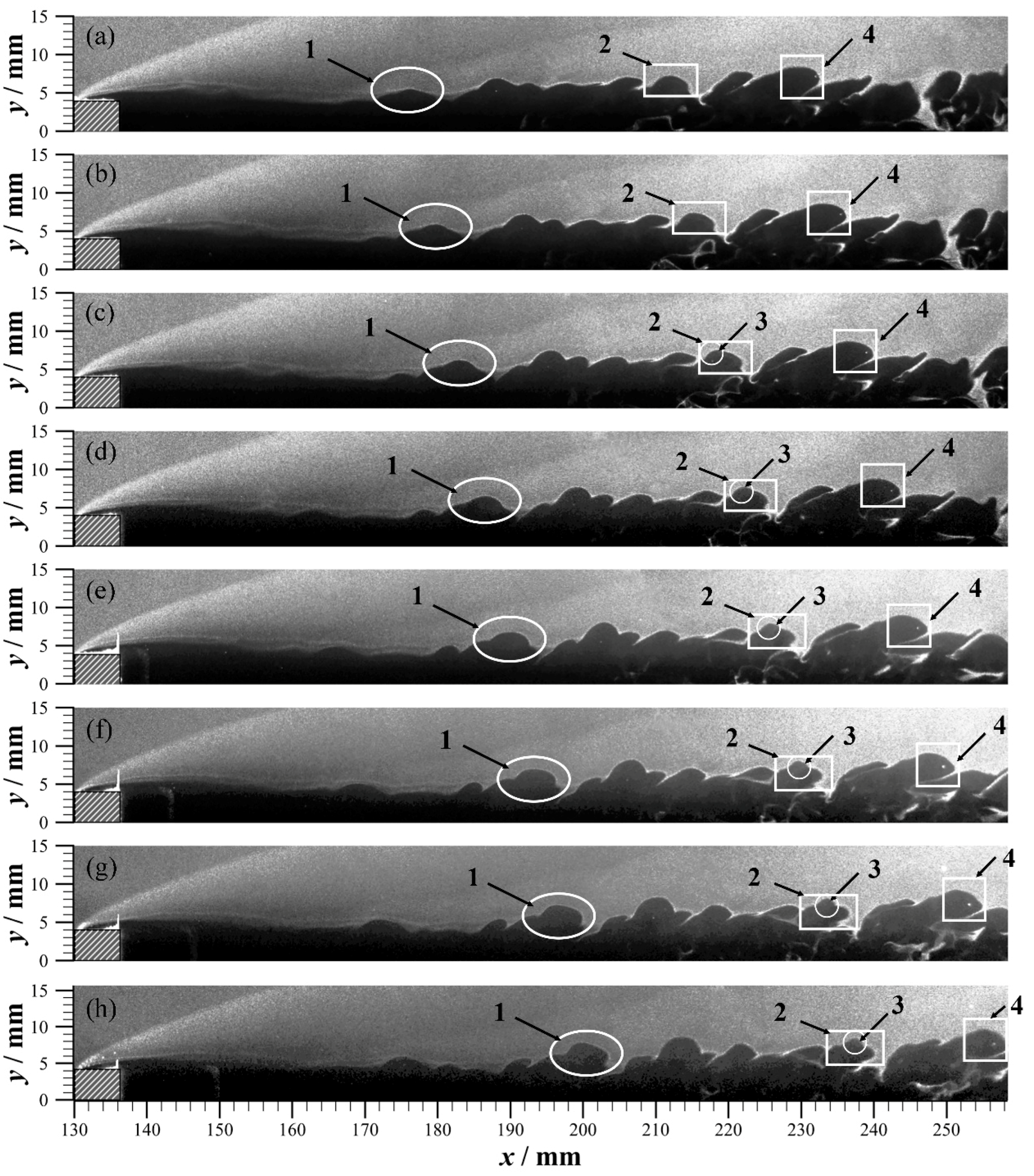
3.4. Time Evolution Characteristic of the Wake Flow Field of a Roughness Element in the xy-Plane

In order to examine the time evolution characteristics of the downstream wake flow field of the roughness element, the time-resolved NPLS technique was exploited to obtain eight time-correlated streamwise image sequences of the wake flow field of the roughness element with k / δ = 2 (see Figure 12). The view field ranged in the following intervals: x = 130 mm–258 mm, y = 0 mm–15 mm, the resolution was 83.3 μm/pixel, and the time interval between adjacent images was 5 μs. The flow direction was from left to right, and the actual unit Reynolds number was 1.37 × 10⁷ m−1.
The evolution process of the wake vortex structure in terms of the flow direction can be observed in Figure 12. The wake vortex structure moved with the flow direction, while a small deformation occurred. Typical vortex structures 1–4 were selected along various flow directions to analyze the dynamic evolution of a single vortex structure in the wake flow. In the elliptical region of Figure 12, vortex 1 was initially a single small protuberance structure. Due to the induction of the horseshoe vortex on both sides, the height of vortex 1 increased continuously in 35 μs. The vortex 1 sheared with the mainstream, exhibited obvious inclination, and formed a clear hairpin vortex structure. The height of the downstream vortex 2 (the rectangular region in Figure 12) was basically unchanged during the time of 35 μs, and its tilt angle was larger than that of vortex 1. At the same time, a new smaller scale vortex structure 3 was induced on the vortex 2, and vortex 3 moved rapidly downstream along the outer boundary of the vortex 2, as presented in the circular region in Figure 12. In the further downstream position, due to the growth of height, the velocity difference between the adjacent vortex structures decreased, the shear effect weakened, the vortex structure remained basically unchanged, and there was no new generated small-scale vortex. This reveals that the vortex structure had developed to a relatively stable state, as vortex 4 in the square region in Figure 12. By analyzing the variations of the overall vortex structure in the wake flow, it is detectable that the farther away from the vortex structure of the roughness element, the stronger the oblique tensile effect is.
In order to further quantify the evolution process of the vortex structure in the wake flow, the average streamwise velocity of vortex 1–4 and the instantaneous streamwise velocity distribution were assessed. Based on the displacements of vortex structures in Figure 12a,h, the average velocities could be extracted, as listed in Table 2. It can be seen from Figure 12a that the height of vortex 1, 2, and 4 magnified gradually. The higher the normal height of the flow structure wall in the boundary layer is, the higher the streamwise velocity is, so the average streamwise velocities of large-scale vortex structures 1, 2, and 4 increased in turn, which is consistent with the results provided in Table 2. The small-scale vortex 3 was induced by vortex 2 while following vortex 2. Although the heights of vortexes 3 and 4 were essentially the same, the average velocity of vortex 3 was higher than that of vortex 4.
Based on the artificial image recognition of the vortex structure, the instantaneous streamwise velocity u of the vortex structure was obtained from the adjacent images. Figure 13 illustrates the instantaneous streamwise velocity distribution corresponding to vortex 1–4 in two adjacent images. The plotted results reveal that the instantaneous velocity of vortex 1 increased with time, which is consistent with the increasing height of vortex 1 in Figure 12. The height of vortex 2 was basically unchanged, and the corresponding instantaneous velocity varied slightly. However, as the structural scale of small-scale vortex 3 increased, its induced effect on vortex 2 made the velocity of vortex 2 relatively lessen, and the velocity of vortex 3 relatively increased. The instantaneous velocity of vortex 4 fluctuated around 730 m∙s−1, equal to 0.93 of the free flow velocity U , which was evaluated to be 786 m/s, as presented in Table 1, which indicates that vortex 4 reached a relatively stable state, which is consistent with the variation of the flow structure observed in Figure 12.
By examining the dynamic evolution process of the vortex structure with various streamwise positions in the wake flow field, it is observable that in the upstream position, it presents the evolution of independent vortex structure, as shown in vortex 1. In the middle position, it developed into the interaction of multiple scale vortex, similar to vortexes 2 and 3. Further downstream, it gradually reached the stable state, and the vortex structure remained basically unchanged, such as vortex 4.

3.5. Comparison of the Wake Flow Field Structure of Roughness Elements with Various Heights

In order to investigate the influence of REH on the wake flow field, the flow structures of roughness element with k / δ = 0.25, 0.5, 0.75, 1.5, 2, and 2.5 were examined. The obtained results are presented in Figure 14. The image shooting range was specified by x = 136 mm–260 mm, y = 0 mm–15 mm, the spatial resolution was 103 μm/pixel, and the flow direction was from left to right. In the experimentation, the actual Reynolds number of each group slightly fluctuated due to the small variation of the incoming flow parameters during the operation of the wind tunnel.
In order to qualitatively compare the influence of the roughness element with various heights on the wake boundary transition, the streamwise position of the first vortex structure in the wake flow was exploited as the basis for comparison and marked with the red vertical line. The distance from the roughness element to the red vertical line was specified as Δl. As presented in Figure 14a, there was no vortex structure in the wake flow field of the roughness element with k / δ = 0.25, which is similar to the smooth plate flow field presented in Figure 7. In the wake flow field of the roughness element with k / δ = 0.5, the first large-scale vortex structure appeared at x = 230 mm, and Δl = 93.7 mm (see Figure 14b). Compared with the roughness element characterized by k / δ = 0.25, the wake boundary layer transition of the roughness element with k / δ = 0.5 occurred earlier. Based on the definition of critical height by Schneider [16], the minimum REH which begins to affect the boundary layer transition is the critical REH. Therefore, the critical REH was less than 0.5 δ under the current flow condition, but it was impossible to determine whether the critical REH was less than 0.25 δ.
As k / δ grew in the range of 0.5–1.5, the position of the first vortex structure in the flow field extended upstream, and the value of Δl lessened from 93.7 mm to 31.7 mm, associated with the red vertical line in Figure 14b–d. Based on the analysis given in Section 3.4, the rapid development of the wake boundary layer was induced by the horseshoe vortex. With the growth of the REH, the vortex structure height in the horseshoe vortex rose, and the inducing effect on the vortex structure in the wake boundary layer was enhanced. As a result, the position of the large-scale vortex structure in the wake boundary layer was closer to the upstream. Compared with Figure 14d–f, it is detectable that the position of the first vortex structure in the wake boundary layer was essentially the same as the growth of the REH with k / δ = 1.5–2.5, and Δl ≈ 30 mm, indicating that the REH had no apparent influence on the position of the large-scale vortex in the current height range.
It should be noticed that the position of the vortex structure in a single image is random, and the distribution law of average streamwise position with the REH cannot be reflected. In order to roughly infer the influence of the REH on the wake boundary layer transition, statistical analysis of flow distance Δl was carried out by 50 images based on the artificial image recognition (see Figure 15a). We used box-and-whiskers plots to perform statistical analysis on 50 samples. In the box-and-whiskers plot, there is a middle line in the box, which denotes the median of the data. The upper and lower bottom of the box represent the upper quartile of the data (Q3) and lower quartile (Q1), which means that the box contains 50% of the data. Q3 and Q1 represent the 75th and 25th data of samples after arranging from small to large, respectively. The discrepancy between Q3 and Q1 is also known as the interquartile range (IQR). Based on the range of 1.5 IQR, the upper and lower edges of the box-and-whiskers plot represent the maximum and minimum values of the set of data. The data of samples outside this range are outliers, as presented in Figure 15a. The plotted results in Figure 15a reveal that Δl lessened from 94 mm to 35.4 mm with the growth of k / δ in the range of k / δ = 0.5–1.5, indicating that the height of the roughness element can apparently promote the wake boundary layer transition. However, as k / δ was higher than 1.5, Δl did not vary remarkably (its value was almost about 40 mm), indicating that the height of the roughness element does not affect the wake boundary layer transition. However, the statistical results obtained from the 50 images may still not be enough to represent the whole population. From the qualitative perspective, it can be considered that 1.5 δ is close to the effective height proposed by Van Driest [9] under the current state, that is, the REH when the transition position extends upstream and is closest to the roughness element.
In order to compare the influence of the REH on the large-scale vortex in the wake boundary layer, the wavelength of the large-scale vortex in a single image was recorded as λ. Further, the ratio of the total wavelength of all large-scale vortex i = 1 n λ i in the image to the number of large-scale vortex n was recorded as the average wavelength λ ¯ (see Figure 14b,c). It is noted from Figure 14 that when the relative REH (i.e., k / δ ) magnified from 0.5 to 1.5, the average wavelength λ ¯ lessened from 13 mm to 5.8 mm, while the relative REH varied in the range of 1.5–2.5, λ ¯ ≈ 6.3 mm, and the average wavelength did not noticeably vary. It is worth mentioning that the scale of the large-scale vortex in a single image is random and the statistical analysis was carried out on the average wavelength λ ¯ by artificially recognizing the 50 images (see Figure 15b). The upper boundary of the error bar represents the maximum of the average wavelength λ ¯ , and the corresponding lower boundary represents the minimum of the average wavelength λ ¯ . As presented in Figure 15b, the average wavelength λ ¯ sharply lessened from 17.63 mm to 7.25 mm with the growth of k / δ in the range of 0.5–1.5, corresponding to the phenomenon that the average wavelength of the vortex structure became smaller and smaller in Figure 14b–d. It is indicated that the REH in this range had an apparent influence on the large-scale vortex in the wake boundary layer. As the relative REH ( k / δ ) reached 1.5, the average wavelength λ ¯ was around 7.75 mm, indicating that for the roughness element with k / δ > 1.5, the REH had no noticeable consequence on the large-scale vortex in the wake flow.
By comparing Figure 15a and Figure 15b, the results reveal that the variation of the flow distance (Δl) and average wavelength ( λ ¯ ) as a function of k / δ as consistent. Compared with the roughness element with k / δ = 0.5, the Δl of the roughness element associated with k / δ = 1.5 reduced by about 62%, and the average wavelength λ ¯ lessened by about 59%. Due to the lessening of the average wavelength λ ¯ of the large-scale vortex structure, the interaction between the vortex was enhanced, which led to the advance of the vortex structure in the flow field and the decrease in the flow distance Δl. For the roughness element with k / δ = 1.5–2.5, the changes of Δl and λ ¯ with the REH were not understandable, indicating that the interaction between the resulted vortexes was stable.
The effect of REH on the boundary layer transition in the wake flow field was scrutinized by implementing the transient image and statistical analysis. The demonstrated results indicate that there was no vortex structure in the image for the roughness element with k / δ = 0.25, and it was impossible to judge its effect on the boundary layer transition, and the vortex structure that appeared in the image was pertinent to the roughness element with k / δ = 0.5. Therefore, the critical REH was less than 0.5 δ, but it was impossible to judge the size between the critical REH and 0.25 δ. For the roughness element with k / δ = 0.5–1.5, the transition position moved forward rapidly with the growth of the REH. By approaching k / δ to 1.5, the position of the first vortex in the wake boundary layer did not noticeably change. The REH had no apparent influence on the transition position, and the effective REH was close to 1.5 δ. Since the boundary layer transition was promoted between the critical REH and the effective REH, it had a trivial effect beyond this range. In the different REHs in this paper, the promoting effect of the boundary layer transition was apparent between 0.25 δ and 1.5 δ, but it was strongly weakened beyond 1.5 δ. As a result, we think that 0.25 δ and 1.5 δ can be employed as reference heights representing the critical REH and the effective REH respectively to provide a basis for the precise prediction and flow control of the boundary layer transition in the current state.

4. Conclusions

In the present paper, the experimental investigation of the wake flow field of isolated roughness element on a Mach 6 plate was performed by employing the flow visualization technique. The transient flow field images of a roughness element with k / δ = 2 in the xy-plane and yz-plane were attained based on the NPLS technique, and the time-correlated transient flow field image sequence of a roughness element with k / δ = 2 in the xy-plane was derived by thetime-resolved NPLS technique. Finally, the transient flow field structures of roughness elements with different heights in the range of k / δ = 0.5–2.5 were appropriately compared.
Combined with the transient flow field images of a roughness element with k / δ = 2 in xy-plane and yz-plane, the gourd-shaped vortex structure initially appeared in the horseshoe vortex, and the appearance of the gourd-shaped vortex structure in the wake flow was later than the horseshoe vortex. The gourd-shaped vortex structure in the wake flow and the horseshoe vortex presented the staggered arrangement. The three-dimensional structure of the flow field was also examined based on the xy-plane and yz-plane images. It was emphasized that the mutual induction mechanism between the horseshoe vortex and the vortex structure in wake flow could lead to the staggered arrangement of the vortex structure.
The dynamic evolution process of the vortex structure in various streamwise positions in the flow field was revealed by time-correlated image sequences. The demonstrated results revealed that the independent vortex structure developed and progressed in the upstream. In the middle stream, the multi-scale vortex interactions developed. In the downstream, the vortex structure gradually reached a stable state and essentially remained unchanged.
The flow structures of the wake flow field of the roughness element with k / δ = 2 were carefully compared. The comparison studies showed that the growth of the REH could promote the wake boundary layer transition when the REH was in the range of 0.25 δ–1.5 δ. For the case of REH lower than 0.25 δ or higher than 1.5 δ, the variation of the REH had no apparent effect on the wake boundary layer transition. Under the current state, the REH of 0.25 δ and 1.5 δ can be rationally employed as reference heights to provide a basis for precise prediction and flow control of the boundary layer transition.
The next work will be focused on the influence of the Reynolds number on the effective height of the roughness element.

Author Contributions

Conceptualization, J.H. and L.H.; methodology, J.H., L.H. and Z.W.; software, J.H., X.X.; validation, J.H., L.H. and X.X.; formal analysis, J.H., L.H.; investigation, J.H.; resources, J.H., X.X.; data curation, J.H., X.X.; writing—original draft preparation, J.H.; writing—review and editing, L.H., X.X. and Z.W.; visualization, J.H.; supervision, L.H.; project administration, L.H.; funding acquisition, L.H. All authors have read and agreed to the published version of the manuscript.

Funding

This research received no external funding.

Data Availability Statement

Not applicable.

Acknowledgments

This work was funded by National Key R&D Program of China (2019YFA0405300), Outstanding Innovative Youth Project of Changsha (KQ2009026), National Natural Science Foundation of China (91752102).

Conflicts of Interest

The funders had no role in the design of the study; in the collection, analyses, or interpretation of data; in the writing of the manuscript; or in the decision to publish the results.

References

  1. Bartkowicz, M.D. Numerical Simulations of Hypersonic Boundary Layer Transition. Ph.D. Thesis, University of Minnesota, Minneapolis, MN, USA, 2012. [Google Scholar]
  2. Kimmel, R. Aspects of hypersonic boundary layer transition control. In Proceedings of the 41st Aerospace Sciences Meeting and Exhibit, Reno, NV, USA, 6–9 January 2003. [Google Scholar]
  3. Lee, C.B.; Chen, S.Y. Recent progress in the study of transition in the hypersonic boundary layer. Natl. Sci. Rev. 2019, 6, 155–170. [Google Scholar] [CrossRef] [PubMed]
  4. Morrisette, E.L.; Stone, D.R.; Whitehead, A.H. Boundary-layer tripping with emphasis on hypersonic flows. In Proceedings of the Viscous Drag Reduction, LTV Research Center, Dallas, TX, USA, 24–25 September 1968; pp. 33–51. [Google Scholar]
  5. Reda, D.C. Comparative transition performance of several nosetip materials as defined by ballistics-range testing. ISA Trans. 1979, 25, 83–98. [Google Scholar]
  6. Berry, S.; Daryabeigi, K.; Wurster, K.; Bittner, R. Boundary-layer transition on X-43A. J. Spacecr. Rocket. 2010, 47, 922–934. [Google Scholar] [CrossRef] [Green Version]
  7. Schneider, S.P. Summary of hypersonic boundary-layer transition experiments on blunt bodies with roughness. J. Spacecr. Rocket. 2008, 45, 1090–1105. [Google Scholar] [CrossRef]
  8. Niu, H.B.; Yi, S.H.; Liu, X.L.; Huo, J.J.; Zheng, W.P. Experimental study of hypersonic traveling crossflow instability over a yawed cone. Acta Astronaut. 2022, 193, 173–181. [Google Scholar] [CrossRef]
  9. Van Driest, E.; McCauley, W.D. The effect of controlled three-dimensional roughness on boundary-layer transition at supersonic speeds. J. Aerosp. Sci. 1960, 27, 261–271. [Google Scholar] [CrossRef]
  10. Whitehead, A.H. Flow-Field and Drag Characteristics of Several Boundary-Layer Tripping Elements in Hypersonic Flow; NASA TN D-5454; National Aeronautics and Space Administration: Washington, DC, USA, 1969.
  11. Bernardini, M.; Pirozzoli, S.; Orlandi, P.; Lele, S.K. Parameterization of boundary-layer transition induced by isolated roughness elements. AIAA J. 2014, 52, 2261–2269. [Google Scholar] [CrossRef]
  12. Borg, M.P.; Schneider, S.P. Effect of freestream noise on roughness-induced transition for the X-51A forebody. J. Spacecr. Rocket. 2008, 45, 1106–1116. [Google Scholar] [CrossRef] [Green Version]
  13. Van Driest, E. Boundary-layer transition at supersonic speeds-three-dimensional roughness effects (spheres). J. Aerosp. Sci. 1962, 29, 909–916. [Google Scholar] [CrossRef]
  14. Braslow, A.L.; Harris, R., Jr.; Hicks, R.M. Use of Grit-Type Boundary-Layer Transition Trips on Wind-Tunnel Models; NASA TN D-3579; National Aeronautics and Space Administration: Washington, DC, USA, 1966.
  15. Sedney, R.; Kitchens, J.C. Measurement and correlation of separation ahead of protuberances in an turbulent boundary layer. In Proceedings of the 14th Aerospace Sciences Meeting, Washington, DC, USA, 26–28 January 1976. [Google Scholar]
  16. Schneider, S.P. Effects of Roughness on Hypersonic Boundary-Layer Transition. J. Spacecr. Rocket. 2008, 45, 193–209. [Google Scholar] [CrossRef]
  17. Chuvakhov, P.V. Controlled experiment on isolated roughness-induced transition in sharp flat plate hypersonic flows. In Proceedings of the AIP Conference Proceedings, Novosibirsk, Russia, 2 November 2018. [Google Scholar]
  18. Wheaton, B.M.; Schneider, S.P. Roughness-Induced Instability in a Hypersonic Laminar Boundary Layer. AIAA J. 2012, 50, 1245–1256. [Google Scholar] [CrossRef]
  19. Wheaton, B.M.; Schneider, S.P. Hypersonic Boundary-Layer Instabilities Due to Near-Critical Roughness. J. Spacecr. Rocket. 2014, 51, 327–342. [Google Scholar] [CrossRef]
  20. Skuratov, A.; Fedorov, A. Experimental investigation of laminar-turbulent transition behind a three-dimensional roughness element in the boundary layer on a sharp cone. Fluid Dyn. 1990, 25, 544–549. [Google Scholar] [CrossRef]
  21. Kuester, M.S.; White, E.B. Structure of turbulent wedges created by isolated surface roughness. Exp. Fluids 2016, 57, 47. [Google Scholar] [CrossRef]
  22. Lash, E.L.; Combs, C.S.; Kreth, P.A.; Schmisseur, J.D. Experimental Investigation of a Cylinder-Induced Transitional Shock Wave-Boundary Layer Interaction. In Proceedings of the 55th AIAA Aerospace Sciences Meeting, Grapevine, TX, USA, 9–13 January 2017. [Google Scholar]
  23. Murphree, Z.; Yuceil, K.; Clemens, N.; Dolling, D. Experimental studies of transitional boundary layer shock wave interactions. In Proceedings of the 45th AIAA Aerospace Sciences Meeting and Exhibit, Reno, NV, USA, 8–11 January 2007. [Google Scholar]
  24. Wang, D.P.; Zhao, Y.X.; Xia, Z.X.; Wang, Q.H.; Huang, L.Y. Experimental investigation of supersonic flow over a hemisphere. Chin. Sci. Bull. 2012, 57, 1765–1771. [Google Scholar] [CrossRef] [Green Version]
  25. Jiang, N.B.; Webster, M.; Lempert, W.R.; Miller, J.D.; Meyer, T.R.; Ivey, C.B.; Danehy, P.M. MHz-rate nitric oxide planar laser-induced fluorescence imaging in a Mach 10 hypersonic wind tunnel. Appl. Opt. 2011, 50, A20–A28. [Google Scholar] [CrossRef] [Green Version]
  26. Zhao, Y.F.; Liu, W.; Xu, D.; Gang, D.D.; Yi, S.H. A combined experimental and numerical investigation of roughness induced supersonic boundary layer transition. Acta Astronaut. 2016, 118, 199–209. [Google Scholar] [CrossRef]
  27. Gang, D.D.; Yi, S.H.; Zhao, Y.X. Experimental and numerical studies of supersonic flow over circular protuberances on a flat plate. Acta Phys. Sin. 2015, 64, 304–311. [Google Scholar] [CrossRef]
  28. He, G.; Zhao, Y.X.; Zhou, J. Visualization of Type IV shock–shock interference induced by a cylindrical protuberance mounted normal to a hollow cylinder. J. Vis. 2020, 23, 9–15. [Google Scholar] [CrossRef]
  29. Sun, T.; Fang, J.Y.; Zhao, D.; Liu, X.; Tong, Q.X. A novel multi-digital camera system based on tilt-shift photography technology. Sensors 2015, 15, 7823–7843. [Google Scholar] [CrossRef] [Green Version]
  30. Zhang, Z.Y. A flexible new technique for camera calibration. IEEE Trans. Pattern Anal. Mach. Intell. 2000, 22, 1330–1334. [Google Scholar] [CrossRef]
  31. Tian, L.F.; Yi, S.H.; Zhao, Y.X.; He, L.; Cheng, Z.Y. Study of density field measurement based on NPLS technique in supersonic flow. Sci. China Ser. G Phys. Mech. Astron. 2009, 52, 1357–1363. [Google Scholar] [CrossRef]
  32. Giepman, R.; Lynch, K.; Schrijer, F.; Van Oudheusden, B. Investigation of a transitional oblique shock wave reflection using PIV. In Proceedings of the 17th International Symposium on Application of Laser Techniques to Fluid Mechanics, Lisbon, Portugal, 7–10 July 2014; pp. 1–17. [Google Scholar]
  33. Li, X.; Bai, B.F. Motion of submicron particles in supersonic laminar boundary layers. AIAA J. 2015, 53, 1037–1047. [Google Scholar] [CrossRef]
  34. Huntley, M.; Smits, A. Transition studies on an elliptic cone in Mach 8 flow using filtered Rayleigh scattering. Eur. J. Mech. B-Fluids 2000, 19, 695–706. [Google Scholar] [CrossRef]
  35. Subbareddy, P.; Bartkowicz, M.; Candler, G. Direct numerical simulation of high-speed transition due to an isolated roughness element. J. Fluid Mech. 2014, 748, 848–878. [Google Scholar] [CrossRef]
  36. Wheaton, B.; Schneider, S.; Bartkowicz, M.; Subbareddy, P.; Candler, G. Roughness-induced instabilities at Mach 6: A combined numerical and experimental study. In Proceedings of the 41st AIAA Fluid Dynamics Conference and Exhibit, Honolulu, HI, USA, 27–30 June 2011. [Google Scholar]
  37. Zhou, Y.L.; Zhao, Y.F.; Xu, D.; Chai, Z.X.; Liu, W. Numerical investigation of hypersonic flat-plate boundary layer transition mechanism induced by different roughness shapes. Acta Astronaut. 2016, 127, 209–218. [Google Scholar] [CrossRef]
  38. Theodorsen, T. Mechanisms of turbulence. In Proceedings of the Second Midwestern Conference on Fluid Mechanics, Columbus, OH, USA, 17–19 March 1952. [Google Scholar]
  39. Theodorsen, T. The Structure of Turbulence. In 50 Jahre Grenzschichtforschung; Vieweg+Teubner: Wiesbaden, Germany, 1955; pp. 55–62. ISBN 978-3-663-19879-6. [Google Scholar]
Figure 1. Hypersonic low noise wind tunnel.
Aerospace 09 00574 g001
Figure 2. Schematic representation of the plate installation.
Aerospace 09 00574 g002
Figure 3. Schematic representation of the roughness element.
Aerospace 09 00574 g003
Figure 4. Schematic representation of the NPLS system.
Aerospace 09 00574 g004
Figure 5. Image comparison with/without TS mechanism: (a) image without TS mechanism, (b) image with TS mechanism.
Aerospace 09 00574 g005
Figure 6. Pixel error distribution of the chessboard corner between camera 2–8 after calibration and camera 1.
Aerospace 09 00574 g006
Figure 7. Transient flow field of the smooth plate in xy-plane (Re = 1.29 × 10⁷ m−1).
Aerospace 09 00574 g007
Figure 8. Transient images of the wake flow field of the roughness element with k / δ = 2 (Re = 1.35 × 10⁷ m−1): (a) flow field image at z = 0 mm in xy-plane, (b) flow field image at y = 3 mm in xz-plane.
Aerospace 09 00574 g008
Figure 9. Staggered hairpin vortex structure.
Aerospace 09 00574 g009
Figure 10. Schematic representation of the hairpin vortex structure in the roughness element wake flow: (a) y = 3 mm, (b) z = 0 mm, (c) x = x0.
Aerospace 09 00574 g010
Figure 11. Schematic representation of the wake flow field at various streamwise positions in xy-plane: (a) x = 150 mm, (b) x = 170 mm, (c) x = 180 mm, (d) x = 190 mm.
Aerospace 09 00574 g011
Figure 12. Wake flow field images of the roughness element with k / δ = 2 (Re = 1.37 × 10⁷ m−1): (a) t = t0, (b) t = t0 + 5 μs, (c) t = t0 + 10 μs, (d) t = t0 + 15 μs, (e) t = t0 + 20 μs, (f) t = t0 + 25 μs, (g) t = t0 + 30 μs, (h) t = t0 + 35 μs.
Aerospace 09 00574 g012
Figure 13. Streamwise instantaneous velocity distribution of vortexes 1–4.
Aerospace 09 00574 g013
Figure 14. NPLS images of the boundary layer flow of the roughness element with various heights: (a) Re = 1.32 × 10⁷ m−1, (b) Re = 1.29 × 10⁷ m−1, (c) Re = 1.41 × 10⁷ m−1, (d) Re = 1.41 × 10⁷ m−1, (e) Re = 1.35 × 10⁷ m−1, (f) Re = 1.32 × 10⁷ m−1.
Aerospace 09 00574 g014
Figure 15. Distribution of Δl and λ ¯ in terms of k / δ : (a) distribution of Δl with k / δ , (b) distribution of λ ¯ with k / δ .
Aerospace 09 00574 g015
Table 1. Mach 6 hypersonic low noise wind tunnel operation parameters.
M a P 0
(MPa)
T 0
(K)
P
(Pa)
T
(K)
R e × 107
(m−1)
U
(m∙s−1)
60.85350538.3642.681.37786
Table 2. Streamwise average velocity of vortexes 1–4.
Vortex 1Vortex 2Vortex 3Vortex 4
U (m∙s−1)690710750730
U / U 0.880.900.950.93
Publisher’s Note: MDPI stays neutral with regard to jurisdictional claims in published maps and institutional affiliations.

