Article

An Improved Synthetic Eddy Method for Generating Inlet Turbulent Boundary Layers

Science and Technology on Scramjet Laboratory, National University of Defense Technology, Changsha 410073, China
*
Author to whom correspondence should be addressed.
Aerospace 2022, 9(1), 37; https://doi.org/10.3390/aerospace9010037
Submission received: 15 October 2021 / Revised: 22 December 2021 / Accepted: 11 January 2022 / Published: 13 January 2022
(This article belongs to the Special Issue Large Eddy Simulation in Aerospace Engineering)

Abstract

:
An improved synthetic eddy method (SEM) is proposed in this paper for generating the boundary layer at the inlet of a computational domain via direct numerical simulation. The improved SEM modified the definition of the radius and the velocities of the eddies according to the distance of the eddies from the wall in the synthetic region. The regeneration location of the eddies is also redefined. The simulation results show that the improved SEM generates turbulent fluctuations that closely match the DNS results of the experiments. The skin friction coefficient of the improved SEM recovers much faster and has lower dimensionless velocity at the outer of the boundary layer than that of the traditional SEM.

1. Introduction

The rapid growth of computation ability has had a great impact on the field of computational fluid dynamics (CFD). The great increase in computational power has brought the possibility of turbulence simulations (LES or DNS) of many complex flow problems. A fully developed turbulent boundary layer is required before the region of interest in the simulation domain or the authenticity of the whole simulation will be affected. A good turbulent inflow needs to be able to faithfully reconstruct all known turbulence information of a specific problem without introducing pseudowaves, independent of the computational grid, geometric configuration and numerical format, and does not affect large-scale parallel computing. Therefore, establishing turbulent boundary conditions is a very challenging task.
The generation methods of turbulent inflow conditions mainly include library-based methods, recycling-rescaling-based methods and synthetic turbulence methods [1,2,3,4]. Library-based methods adopt the turbulence library from experiments or DNS results. The phase information of the fluctuations can be well restored by library-based methods due to the reality of the turbulence library from experiments or DNS results [5]. However, these methods rely on periodically reading the library during the iterations. Periodic fluctuations may be generated in the streamwise direction if it is not treated well, and it is usually not easy to obtain the libraries corresponding to the calculation conditions. Therefore, library-based methods are rarely used now.
Recycling-rescaling-based methods generate turbulent inflow conditions by readjusting the velocity field downstream and reintroducing the velocity field at the inflow. Different similarity laws are used to rescale the mean velocity and fluctuations in the inner and outer regions of the boundary layer [6]. This method has a good application in the calculation of straight flow fields [7,8,9], but it is difficult to calculate the flow field with complex configurations. In addition, this method involves the correlation between a plane inside the flow field and the inlet plane, which will carry out additional communication in parallel calculations.
The simplest idea of the synthetic turbulence methods is to superimpose the desired average velocity distribution and random white noise on the inlet. However, due to the lack of any spatial or temporal coherence, the fluctuations generated by this simple method usually disappear within a short distance downstream [10]. Therefore, spatial and temporal coherence is added in practical synthetic turbulence generators to restrain fluctuations. The most common applications are the digital filter method [11] and synthetic eddy method [10]. The digital filter method establishes a digital filter of the Gaussian two-point correlation function. The filtered random signal has the required spatial length scale and can be further transformed to meet the specified Reynolds stress tensor. After continuous improvement, this method has been applied to many academic problems. Its obvious disadvantage is that the filtering operation is mainly suitable for finite difference separation and discretization using uniformly spaced Cartesian structured grids, which will be difficult in the application of complex configurations such as circular inlets.
In the synthetic vortex method, the superposition of coherent structures is simulated by introducing artificial eddies (the word “eddy” refers specifically to artificial eddies in the paper) into the inlet plane. Each eddy is a vorticity source with a three-dimensional structure represented by a specific shape function describing its spatial and temporal characteristics [12]. The velocity fluctuations at a given grid point on the inlet plane are calculated by superimposing the effects of all eddies. The synthetic eddy method has the advantages of the synthetic turbulence method; that is, it does not depend on the database, and vortex points do not depend on a specific grid, so it is easy to use in complex configurations and has no additional cost for parallel computing. Therefore, the synthetic eddy method is currently the mainstream generation method of turbulent inflow conditions.
Jarrin et al. [12,13] proposed the original SEM based on the principle of the vortex method. The core idea of the SEM is to generate turbulence through a series of eddies that satisfy the nondivergence condition. The spatial and temporal correlations of the turbulent structure are restored by the superposition of random pulsations and the flow directions of different eddies. SEM has been widely utilized and continuously improved since it was proposed. Pamiès et al. [14] used information in the available literature about the coherent structure in the turbulent boundary layer to design a shape function to simulate the vortex strip in the near-wall region and a hairpin vortex in the logarithmic layer and wake region. Poletto et al. [15] developed a nondivergent SEM by modifying the shape function for the action range of eddies. Tabor et al. [16] compared the recycling/rescaling method and SEM, analyzed their advantages and disadvantages, and reported that SEM is more flexible. Mankdadi [17] implemented the SEM and numerical filtering method based on the LES technique and discovered that the SEM can better reproduce the experimentally obtained turbulent stress. Lee et al. [18] used the turbulent kinetic energy at the corresponding position of each eddy to replace the Reynolds stress; accordingly, the turbulent kinetic energy and velocity time-averaged profile can be obtained by the Reynolds-averaged Navier–Stokes (RANS) equations, thereby reducing the difficulty in obtaining the Reynolds stress.
Several practical problems are found in our application of SEM:
  • The traditional SEM seems to overestimate the eddy radii in the near wall region. The radii reach the maximum 0.41 δ ( δ is the boundary layer thickness) at the approximate position of 0.2 δ . The grids near the wall will be affected by too many eddies, which cause much larger vortex structures to be generated than small vortex structures. In the compressible LES study of Mankbadi et al. [17], it is found that SEM could succeed in replicating the Reynolds stress tensor when the radii of the eddies are taken as 0.1 δ after a preliminary boundary layer study where the radii were varied, while the moving speed of the eddies is 0.5 U . This also indicated overestimates of the eddy radii in the near-wall region. Detailed comparisons of the radii can be seen in Section 3.
  • The velocity of the actual vortex structures should be close to the average velocity of the turbulent boundary layer. The velocity of vortex structures in the near wall region is much lower than that in the outer layer of the boundary layer. Therefore, it is unreasonable to set all the eddy moving velocities as the mainstream velocity U . This may be the reason Mankbadi et al. [17] chose 0.5 U eddy moving velocities.
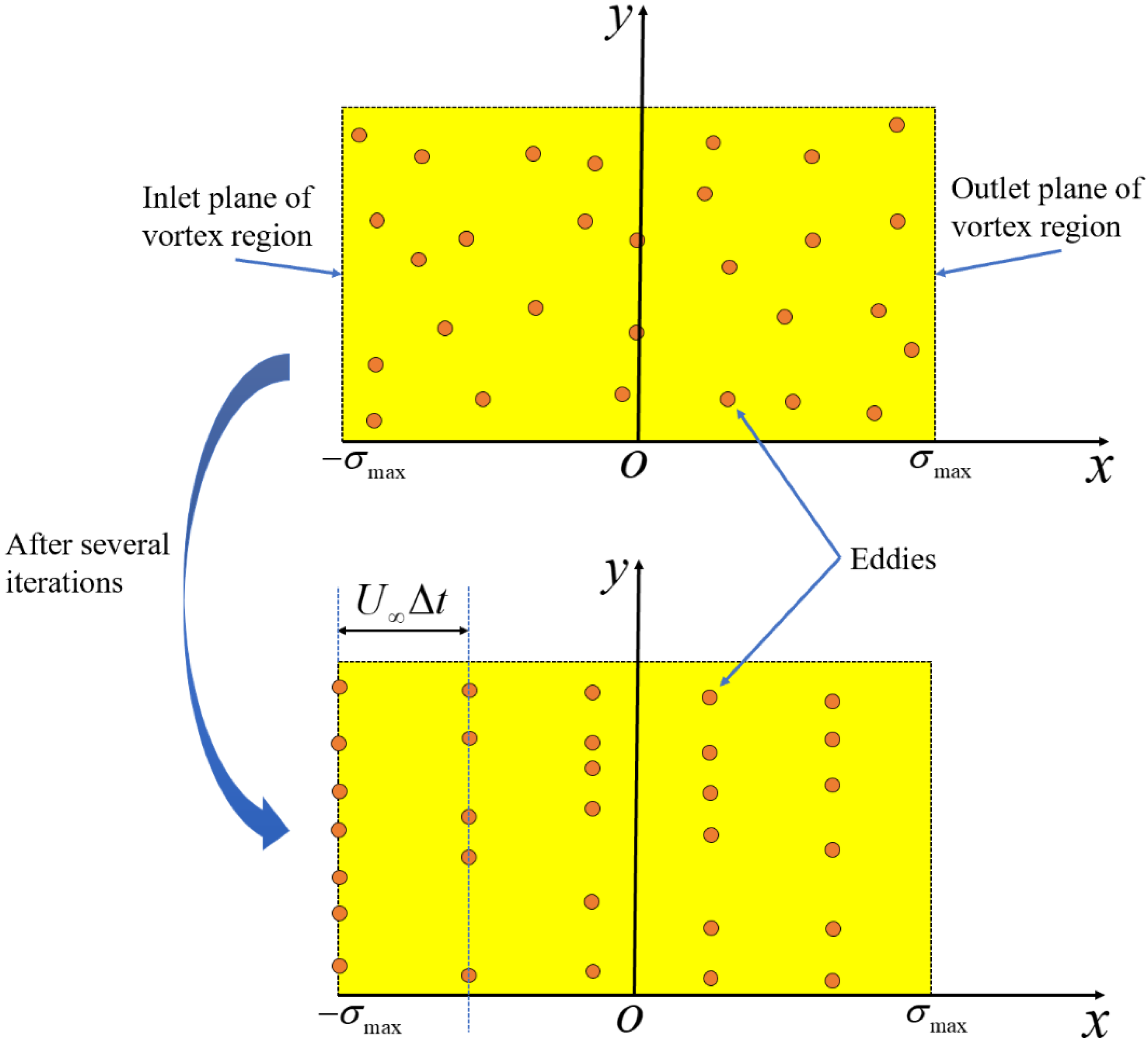
  • The vortex points are evenly distributed in the eddy region at the first step, and the vortex points leaving the outlet plane of the eddy region are regenerated on the inlet plane of the vortex region, which means x k n = σ max . This will cause a problem. After several or more steps, the streamwise distribution of the vortex will be sorted to several points at a time step away, thus losing the randomness of the flow direction, which is shown in Figure 1.
Considering these shortcomings, this paper studies the parameters of a supersonic turbulent boundary layer with Ma = 2.7 to propose a set of easy-to-use SEM applications. Part 2 briefly explains the basic principle of the SEM, Part 3 presents the specific details of the improved method, and finally, in Part 4, the method is applied to generate the turbulent boundary layer at the entrance of a flat plate to demonstrate the effectiveness of the proposed method.

2. Numerical Methods

2.1. NS Code

The simulations are run within an in-house GPU-based 3D unsteady compressible NS equation solver; more details about the code can be found in the literature [19].
A low-dissipation fourth-order hybrid of the central/WENO scheme is used for inviscid fluxes. An energy-preserving central difference scheme is used for the central difference scheme. In terms of the fourth-order energy-conservation scheme, the semidiscretizations of the numerical approximations are:
f i + 1 / 2 E C = 1 48 ( ρ i + 2 + ρ i ) ( u i + 2 + u i ) ( φ i + 2 + φ i ) + 7 ( ρ i + 1 + ρ i ) ( u i + 1 + u i ) ( φ i + 1 + φ i ) + 7 ( ρ i + ρ i ) ( u i + u i ) ( φ i + φ i ) ( ρ i 1 + ρ i ) ( u i 1 + u i ) ( φ i 1 + φ i )
where φ stands for a generic transported scalar property, being unity for the continuity equation or u k for the momentum equations or H = γ γ 1 p ρ + u 2 2 for the total energy equation.
Central-upwind fourth-order WENOCU4 scheme for the WENO scheme. It is defined as:
f ^ i + 1 / 2 W E N O = k = 0 r 1 ω k f ^ k , i + 1 / 2 , k = 0 , 1 , 2
where:
ω k = α k k = 0 2 α k , α k = d k C + τ 3 β k + ε , k = 0 , 1 , 2
d 0 = 1 6 , d 1 = 2 3 , d 2 = 1 6
where ε is a small positive value to prevent the denominator from becoming zero and β k is the smoothness indicator, which can be given by:
β 0 = f i 1 + f i 2 β 1 = f i + f i + 1 2 β 2 = f i + 1 + f i + 2 2 β 3 = 1 36 2 f i 1 3 f i + 6 f i + 1 f i 2 2 + 13 12 f i 1 2 f i + f i + 1 2 + 781 720 f i 1 + 3 f i 3 f i + 1 + f i + 2 2
where f ^ k , i + 1 / 2 represents the substencil fluxes obtained from the node value f i as:
f ^ 0 , i + 1 / 2 = 1 2 f i 1 + 3 2 f i f ^ 1 , i + 1 / 2 = 1 2 f i + 1 2 f i + 1 f ^ 2 , i + 1 / 2 = 3 2 f i 1 1 2 f i + 2 f ^ 3 , i + 1 / 2 = 1 12 f i 1 + 7 12 f i + 7 12 f i + 1 1 12 f i + 2
τ 3 is the reference smoothness indicator as:
τ 3 = β 3 β 0 + β 1 2
The hybrid algorithm is that the shock-capturing WENOCU4 scheme is only activated near critical cells, while the fourth-order energy conservation scheme is employed for the other flow field with smooth scales. Then, the hybridization is devised as:
f ^ i + 1 / 2 = 1 ψ f ^ i + 1 / 2 E C + ψ f ^ i + 1 / 2 W E N O
where the weighting function ψ is defined as:
ψ = 1 ,   if   θ > ξ 0 ,   otherwise
where ξ controls the sensitivity to identify the critical regions, which depends on the stability of the program. Generally, we have ξ = 0.98 in our application to simulate the supersonic boundary layer. The shock sensor θ can be calculated by the nonlinear weight of the substencils. The formula is defined in Equation (10).
θ = l = 0 3 ω l / d l 1 2 1 / min d m 1 2 + 3 , l , m = 0 , 1 , 2
The diffusive term adopts a fourth-order central difference scheme. The time integration scheme uses the third-order explicit Runge–Kutta method.

2.2. Theory of the SEM

Jarrin et al. [12,13] systematically described the implementation of the SEM. The basic theory of the traditional SEM is briefly described here.
First, a synthetic eddy region (ER), shown as Figure 2, a box region symmetrical about the entrance plane, is established near the inflow boundary of the computational domain, as shown in Figure 2. Enough virtual eddies are scattered in this region. The bottom wall of this synthetic region is a nonslip boundary, and the height of the top boundary is greater than the thickness of the turbulent boundary layer. In addition, the thickness of the synthetic region is the double maximum of the radium of the eddies.
The eddies within the ER do not possess a physical vortex structure and are used to generate a random process to simulate the randomness of velocity fluctuations. Furthermore, these eddies have a fixed radius, which is usually comparable to the average grid scale or slightly smaller than the maximum grid scale within the boundary layer. The eddies affect the magnitude of the pulsations on the grid points located within their radii.
The time-averaged flow velocity at each grid point is first determined according to its distance from the wall, and its final velocity is the sum of this time-averaged velocity and the velocity fluctuations. Specifically, the effects of the eddies that can disturb the grid point are superimposed, and this superposition yields a value that quantifies the total disturbance effect, which is eventually fed back to the velocity fluctuations with the help of the known Reynolds stress corresponding to the velocity fluctuations at the grid point.
In general, the eddies are evenly distributed in the synthetic eddy region so that each grid point can be disturbed by a certain number of eddies as long as the number of eddies is guaranteed to be sufficiently large. Figure 3 presents a schematic representation of the movement of a certain eddy, which moves forward with the incoming flow at a certain speed that is often set as a constant in the numerical simulation.
The movement of the eddies is described as follows:
(1)
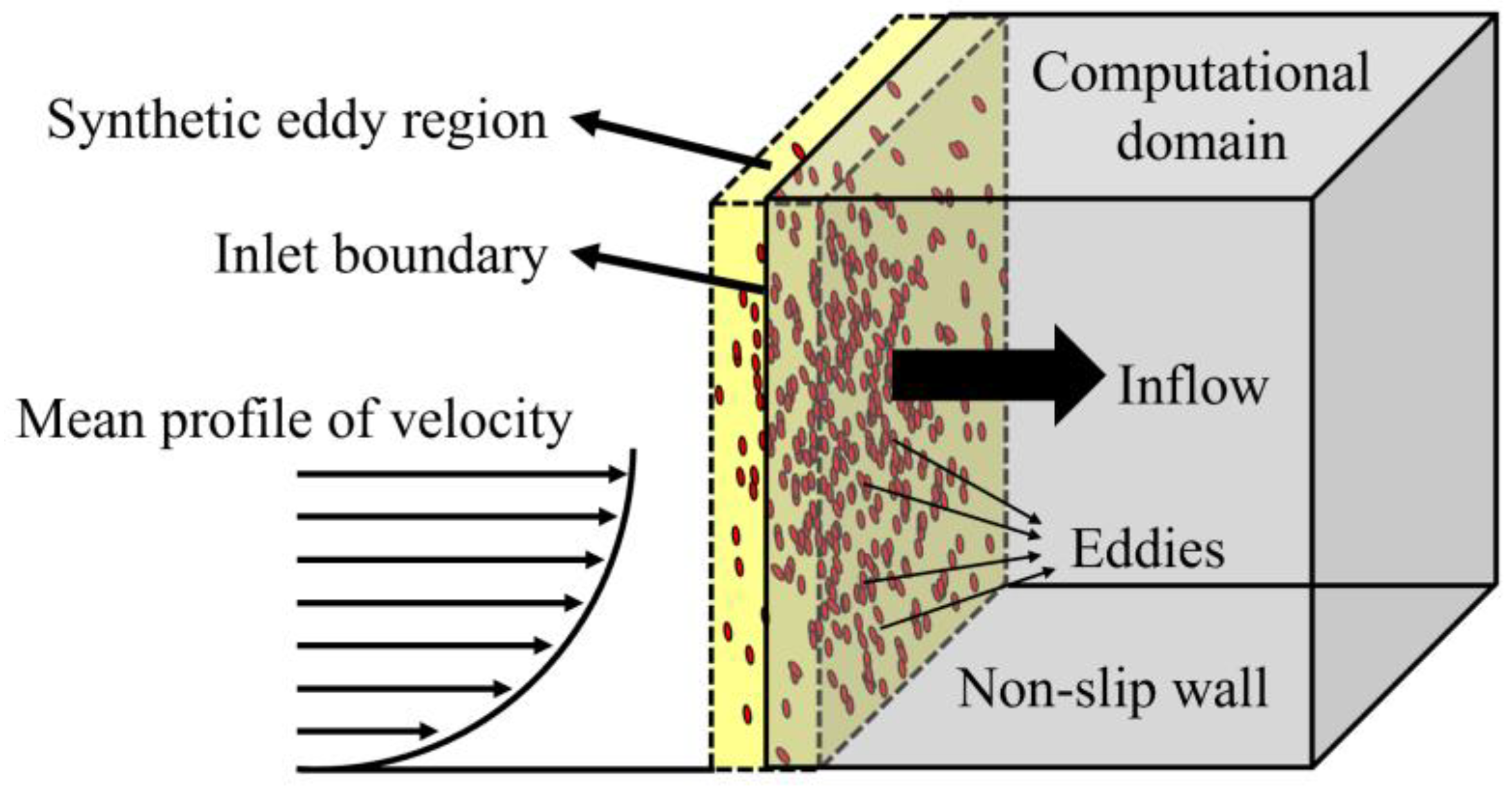
The eddies are evenly initialized in the synthetic vortex region with a certain radius and carry random information that can influence the generation of turbulent fluctuations at the first iteration. All information about the eddy k can be expressed as x k , y k , z k , ε k , σ k , U k , where x k , y k , z k is the initialized location in the synthetic vortex region, ε = r a n d o m ( ± 1 ) x , r a n d o m ( ± 1 ) y , r a n d o m ( ± 1 ) z determines the directions of the velocity fluctuations, and σ k and U k are the radius and the moving velocity of the eddy, respectively. All the eddy information remains unchanged until the eddy regenerates, except x k .
The profile of the radii of the eddies proposed by Jarrin et al. [12] is:
σ 1 = max min L t , 0.41 δ , Δ max
where the integral turbulence length scale is L t = k 3 2 ε , k is the turbulence kinetic energy, ε is the dissipation rate, and Δ max is the max grid of the inlet.
The eddies constantly move downstream with the numerical iteration process with the velocity U k = U . Therefore, at each iteration, the new position of eddy k is given by x k t + Δ t = x k t + U Δ t .
(2)
The eddies in motion disturb the grid points within their radii, affecting the generation of velocity fluctuations. The velocity of a grid point on the inlet boundary can be expressed as:
u i = U ¯ i + u i
where i represents the three spatial directions, U ¯ i is the time-averaged velocity, and u i is the pulsation velocity.
The total number of small vortices is set to N = max V / σ 3 , where V is the volume of the eddy region. Then, the pulsation velocity can be calculated by the following equation:
u = 1 N k = 1 N a i j ε k f ( x , y , z , x k , y k , z k , σ k )
where k represents the sequence of the eddies, a i j signifies the Cholesky decomposition values of the turbulent Reynolds stress tensor at the grid points, and the Reynolds stress tensor mentioned herein refers to the matrix of the second-order pulsation velocity:
R i j = u u u v u w u v v v v w u w v w w w
f x , y , z , x k , y k , z k , σ k is a decay function of eddy x k , y k , z k at grid point x , y , z . This function has the following characteristics: if the grid point is within the radius of the eddy, f > 0 ; otherwise, f = 0 . f is defined as follows:
f x , y , z , x k , y k , z k , σ k = V σ k 1 / 3 ψ x x k σ k ψ y y k σ k ψ z z k σ k
where V e is the volume of the synthetic eddy region and ψ is defined as:
ψ θ = 3 2 1 θ ,   θ < 1 0 , θ 1
where θ = x x k σ k , y y k σ k , z z k σ k , respectively.
(3)
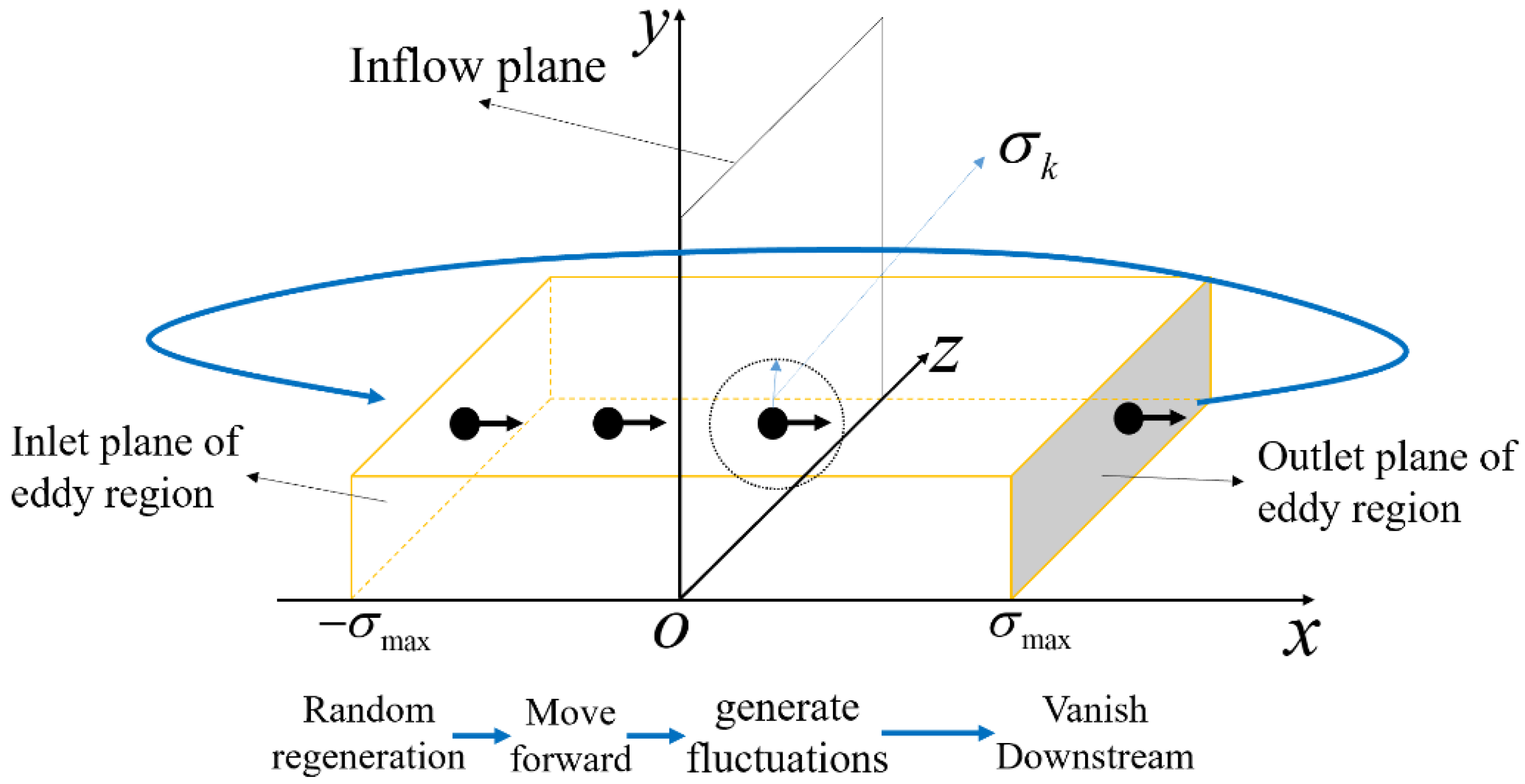
Once an eddy escapes from the outlet plane of the synthetic eddy region, it is regenerated randomly in the inflow plane synthetic vortex region to keep the total number of eddies constant, which can be given as:
x k t y k t z k t Δ t if   x k t + Δ t > σ max x k t + Δ t = σ max y k t + Δ t = random ( y k ) z k t + Δ t = random ( z k )
As long as the effects of eddies are similar enough to the natural random process, the fluctuations generated by the eddies are capable of reconstructing the turbulence characteristics of the boundary layer of the flow.

3. Improved SEM

Due to the shortcomings, we modified the original SEM.
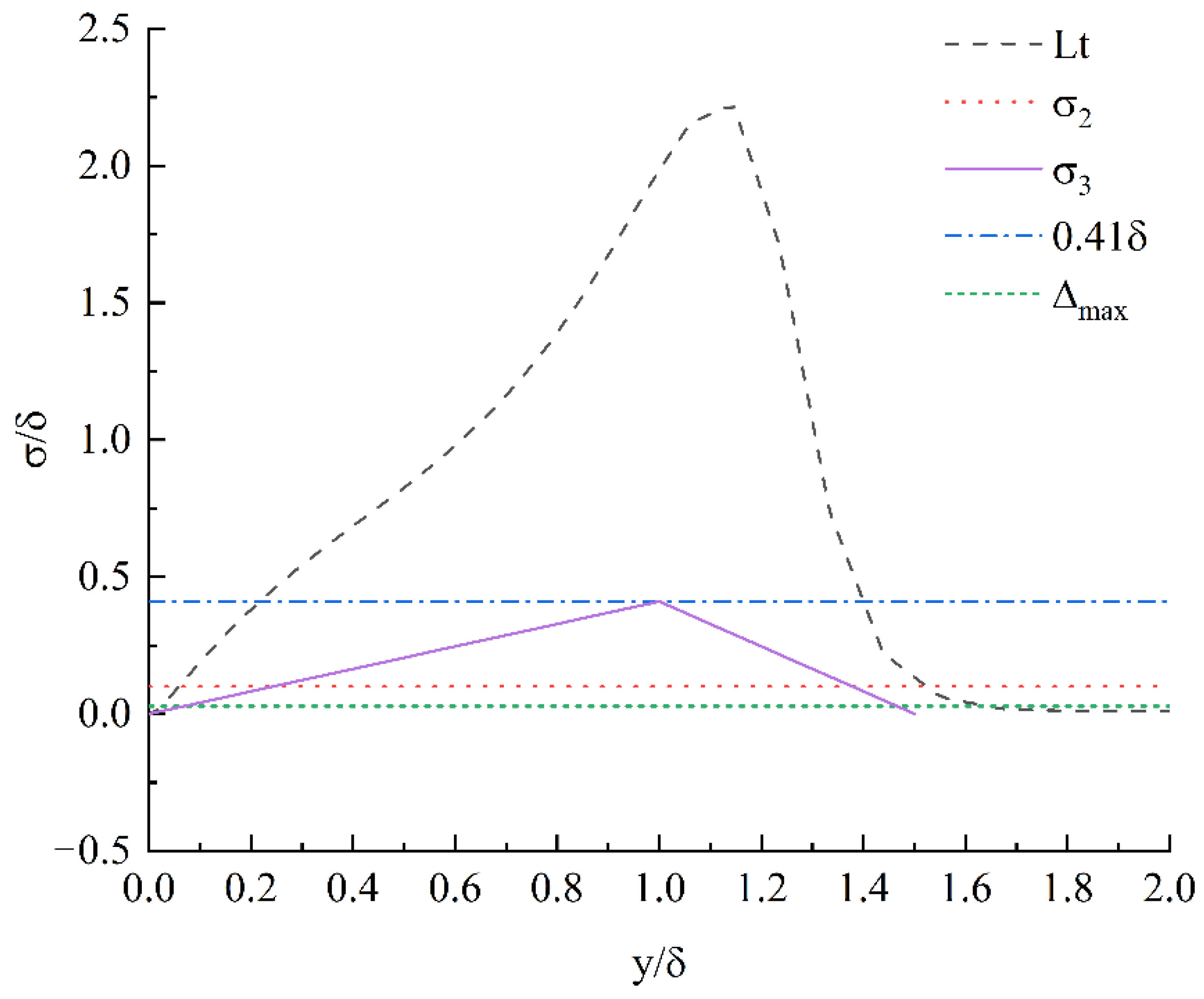
  • The radius profile of eddies is shown as σ 3 in Figure 4. It is defined as:
    σ 3 = max 0.41 y w , Δ max , y w < δ max 0.82 y w + 0.41 δ , Δ max , y w δ
    where y w is the distance of the eddies to the wall. The linear distribution along the wall normal direction is adopted. We also tried the velocity distribution of a velocity profile shape, which was slightly different from the linear distribution. Therefore, we use the linear distribution for ease of use. The profile σ 2 = 0.1 δ is adopted by Mankbadi et al. [17]. Compared with the profile of the radii of the eddies proposed by Jarrin et al. [12], the profile proposed in this paper reduces the eddy radii near the wall, while it is closer to that proposed by Mankbadi et al. [17].
With the change in radius, the total number of eddies can be calculated as follows: First, an average radius is defined:
σ e = y = 0 δ σ y d y / δ 0.2 δ
Then, the total number of eddies is approximately determined as:
N = V e σ e 3
2.
The moving velocity of the eddies adopts the average velocity of the turbulent boundary layer. However, to avoid the parallel efficiency loss caused by the interpolation of the velocity of the eddies regenerated in each iteration, an approximate expression U x = ( y w / δ ) 1 / 7 U [20] of the velocity profile is adopted. Therefore, the position of each eddy is updated after a time step Δ t
x k t + Δ t = x k t + U k y k Δ t
y k and z k remain constant before the eddy vanishes.
3.
The new positions of the eddies are set as follows when the streamwise positions of the eddies are greater than σ max
x k t y k t z k t Δ t if   x k t + Δ t > σ max x k t + Δ t = x k t 2 σ max y k t + Δ t = random ( y k ) z k t + Δ t = random ( z k )
For the temperature and density, the improved SEM correlates them with velocity fluctuations by a strong Reynolds analogy:
T T ¯ = γ 1 M a ¯ 2 u U ¯
The pulsation density is then obtained with the ideal gas equation of state ρ / ρ ¯ = T / T ¯ , where T ¯ , M a ¯ sand ρ ¯ are the local time-averaged temperature, Mach number and density, respectively.

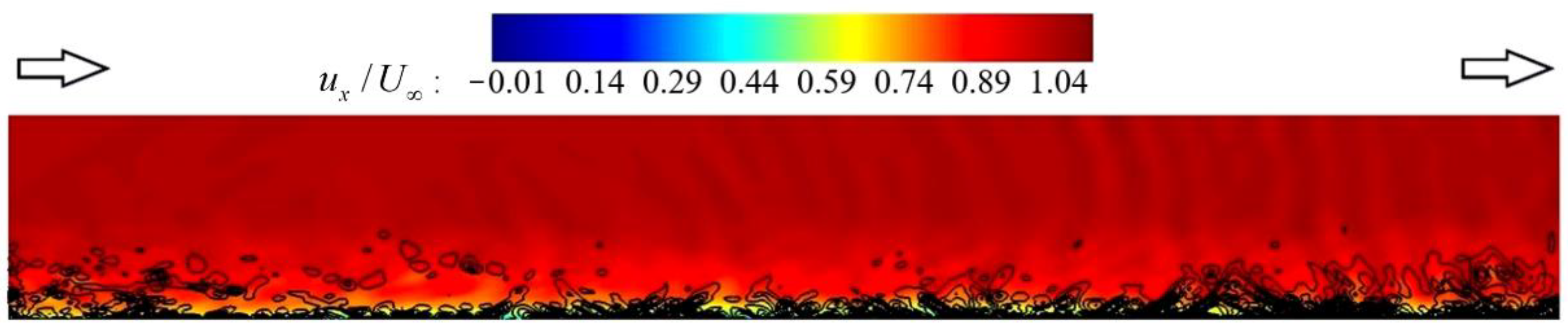
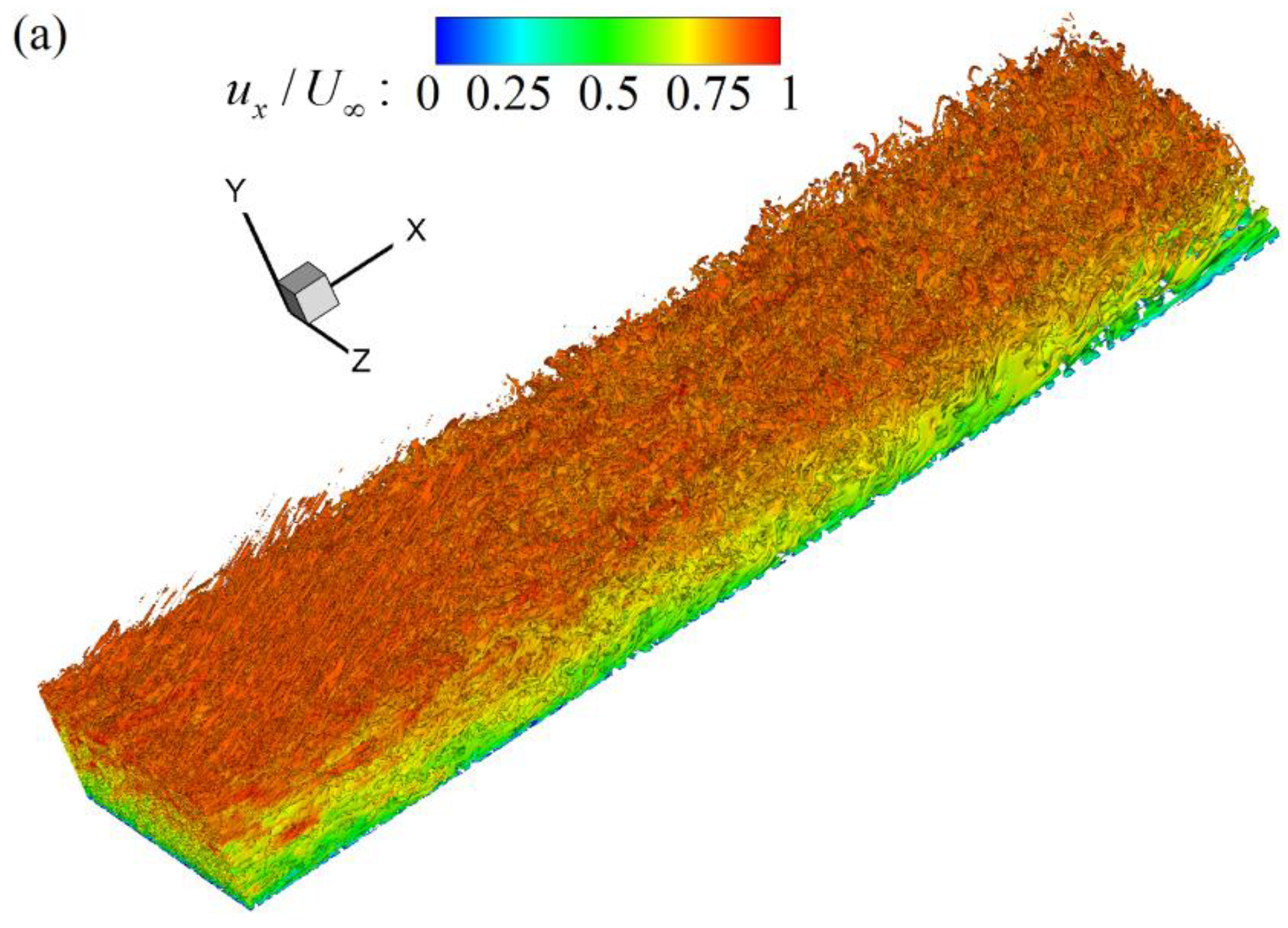
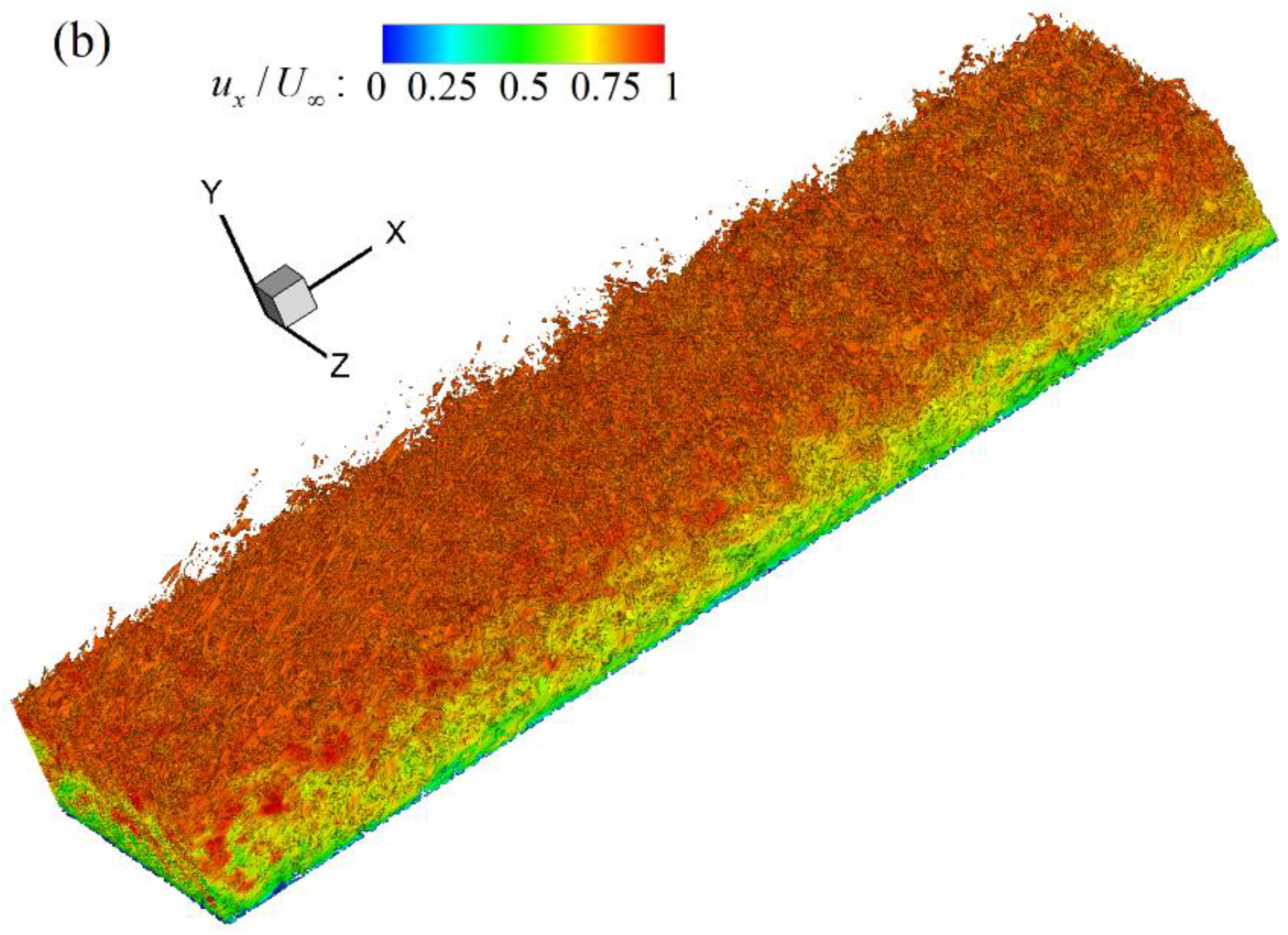
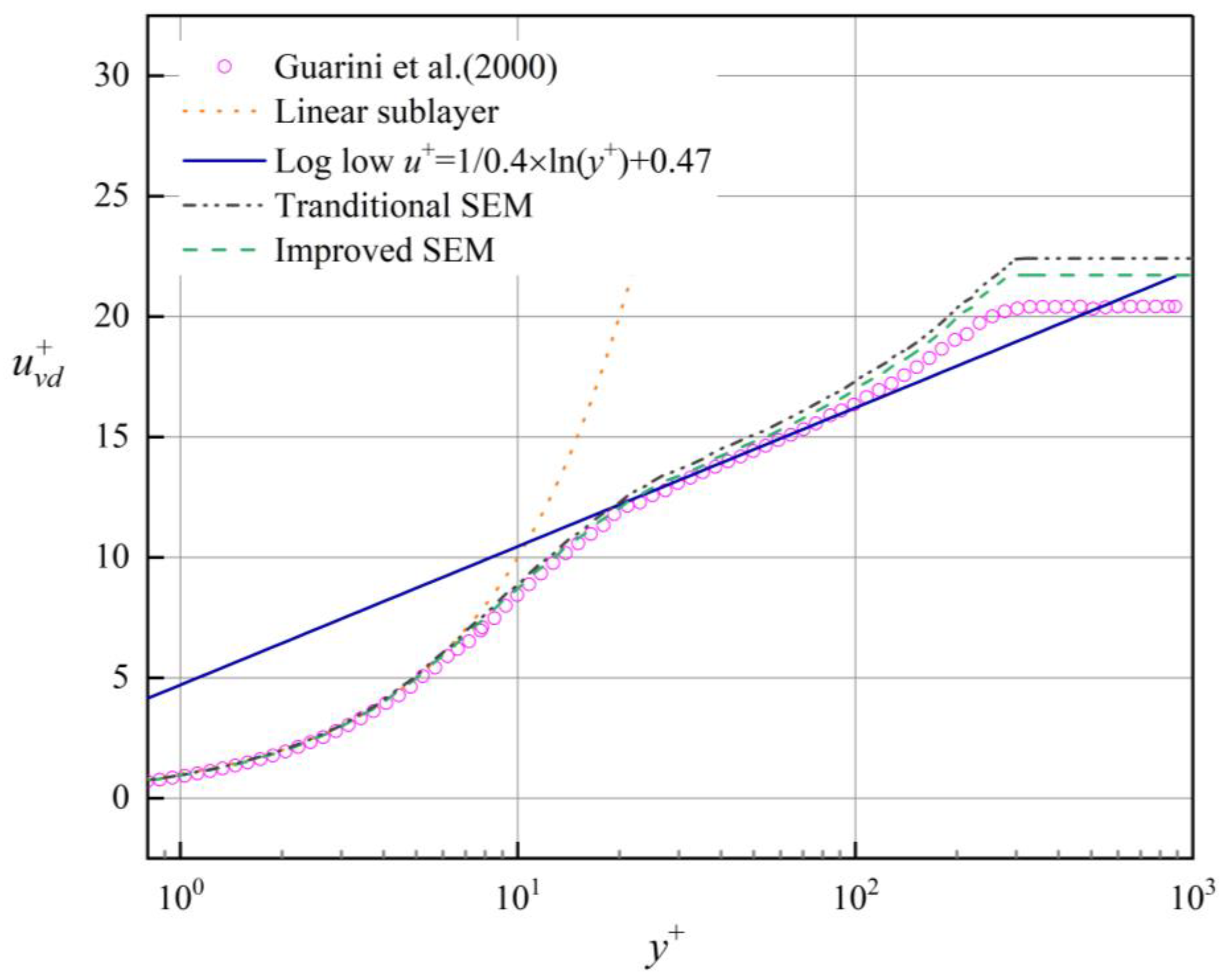
4. Application of the Improved SEM to a Supersonic Plate Flow

This paper obtains the results of the DNS [1] of the turbulent boundary layer of a plate with M a = 2.52 , from which the Reynolds stress tensor components are extracted, as shown in Figure 5. Since the Reynolds shear stresses u v , u w and v w are small compared to the main diagonal elements of the tensor, to conserve memory and reduce the computational overhead, it is assumed that u w and v w have the same distribution as u v .
The computational domain is shown in Figure 6. A fine mesh of 473 × 360 × 270 grids is used for the current simulation as shown in Table 1. To minimize artificial reflections from the boundaries, large buffer regions (2.7 times the boundary layer thickness, as shown in Figure 6) are introduced on both the side boundaries and the upper boundary. The streamwise and spanwise grids are evenly distributed. In the wall normal direction, the mesh has 21 evenly distributed grid points near the wall as the inner mesh with a resolution of y + = 1 , 191 grid points stretch from the inner mesh to 0.6 δ , 121 grid points are evenly distributed from 0.6 δ to 1.5 δ , and the rest stretch to the up boundary. The outlet of the computational domain is set as the supersonic outlet, and the thickness of the boundary layer is set to δ = 1.8 mm.
Two simulations are carried out in this paper based on the mesh. The program can run stably when the time step is 4 × 0−10 s, while the corresponding Courant number is approximately 0.5.
The average statistical characters are counted after 300,000 time steps (two overall flow times), and another 150,000 time steps are counted for the statistical characters (one overall flow time). Every step is counted. Both cases are treated with the same methods.
To examine the generation of pulsations at the inlet boundary for the improved SEM, the contours of the flow pulsation velocity at the inlet boundary monitored with the time step are plotted in Figure 7. To clearly distinguish the pulsation velocity direction, red represents a positive pulsation, and blue represents a negative pulsation. The area marked by the black dashed circle in each panel reflects the evolution of a positive pulsation velocity occurring in this series of consecutive moments. The direction and amplitude of the inlet velocity fluctuations are physically realistic based on the continuous forward motion of the eddy. On the other hand, the overall distribution of positive and negative velocity fluctuations in the boundary layer is statistically homogeneous owing to the random dispersion of the eddies, although the characteristic scale of these pulsations varies significantly at different heights.
Figure 8 shows the contours of the transient vortex distribution colored by the local density. The vorticity is concentrated mainly near the wall. The distribution of these vortex contours further reveals the difference between the bottom layer and the outermost layer of the turbulent boundary layer: in the region close to the wall, where the nonslip viscosity of the wall plays a major role, there are many small, closed vortex contours, while the upper region consists mostly of a long strip-like structure split by the strong shear effect of the main flow and the boundary layer. Moreover, the density distribution exhibits a phenomenon where the pulsation density is strongest at the entrance and then gradually weakens downstream. This may be because the pulsation density distribution given by the SEM is not physically realistic near the entrance but is constantly corrected downstream by the flow itself before finally returning to the proper pulsating state.
Figure 9 visualizes the transient dimensionless flow velocity contours and the second invariant of the velocity gradient tensor along the spanwise center section. The second invariant of the velocity gradient tensor is defined as:
Q = 1 2 u i x j u j x i
which theoretically characterizes the relative equilibrium between the vortex strength and the local shear stress rate. Q provides an intuitive indication of the vortex structure in the flow field. The development of the vortices along the stream is not uniform; for instance, the vortices in the outermost boundary layer go through a process of disappearing and then gradually regenerating. In particular, the velocity distributions of the flow in the boundary layer and the main flow area can be observed from Figure 9. Due to the pulsation of the velocity in the boundary layer, the main flow fluctuates along the upper edge of the boundary layer, and this fluctuation, which originates in the shear region near the inlet between the main flow area and boundary layer, propagates downstream in the main flow.
Figure 10 shows the isosurfaces of the 3D structure of Q colored by the instantaneous streamwise velocity. In both cases, the turbulence structures introduced at the inflow boundary are adjusted to some degree, causing the turbulence to initially decay. This decay is followed by an increase in turbulence as the turbulent boundary layer tends toward equilibrium. The isosurfaces demonstrate that the adjustment distance generated by the traditional SEM is longer than that generated by the improved SEM.
The mean velocity distributions at x = 12 δ are shown in Figure 11. The profiles are transformed with
u + = u u τ
and scaled with ρ / ρ w :
u v d + = 0 u + ρ ρ w d u +
The density-weighted transformation method was developed by van Driest [21] for compressible fluids. The wall-normal coordinate is transformed according to:
y + = y u τ υ w
Figure 11 plots the profiles obtained with the traditional SEM and improved SEM and from the DNS by Morgan et al. [1]. The profile acquired with the traditional SEM is almost the same as that with the improved SEM but deviates from the linear sublayer profile and is slightly higher than the log layer profile. A larger velocity is obtained with the traditional SEM along the wall at the edge of the boundary layer due to the underestimation of u τ with the traditional SEM. The current simulation results are very consistent with those obtained by the DNS conducted by Morgan et al. [1].
The skin friction coefficient is defined as:
C f = μ w d u 1 d y 1 / ( 0.5 ρ U 2 )
In the simulation the skin friction coefficient was found to be C f 0.00273 with the improved SEM and the corresponding Reynolds number based on the momentum thickness Re θ = 1456. The simulation compares favorably with the experimental results compiled by Coles (1954) and the skin friction correlation given in Bardina, Huang and Coakley (1997) based on the Van Driest II skin friction transformation in Figure 12. The streamwise skin friction coefficients are shown Figure 13. After experiencing a very similar trough, the C f of the improved SEM rose more rapidly than the traditional SEM. Finally, the restored C f of the improved SEM is slightly larger, which may be the reason for the lower velocity profile of the outer boundary region.
Further quantitative comparisons can be achieved by calculating the root mean square values of the pulsation velocity at the downstream exit boundary.
The root mean square values of the time-averaged pulsation velocity at x = 12 δ calculated by the traditional SEM (total number of small eddies N = 4000) and the improved SEM are compared with the values extracted from the DNS results in Figure 14. For the same number of small eddies, the traditional SEM underestimates the longitudinal pulsation velocity within the boundary layer, especially in the interior of the boundary layer ( y / δ < 0.2 ). The improved SEM, on the other hand, restores the DNS results relatively well.

5. Conclusions

In this paper, direct numerical simulations of a supersonic turbulent boundary layer are carried out for a freestream Ma of 2.52. An improved SEM method for generating turbulent boundary layers is proposed. Three corrections have been made on the basis of the traditional SEM:
(1)
The velocities of the eddies are redefined according to the distance of the eddies from the wall in the synthetic eddy region, as the traditional SEM overestimates the eddy radii in the near wall region.
(2)
The moving velocity of the eddies adopts the average velocity of the turbulent boundary layer. An approximate expression, U x = ( y w / δ ) 1 / 7 U [20], of the velocity profile is adopted to avoid velocity interpolation.
(3)
Regenerated streamwise coordinates of the eddies in the synthetic eddy region are also modified to avoid random reduction.
The improved SEM is more effective than the traditional SEM in the simulation of the supersonic boundary layer flow along the wall of a flat plate. The skin friction coefficient of the improved SEM recovers much faster and has lower dimensionless velocity at the outer of the boundary layer than that of the traditional SEM. The improved SEM needs a shorter distance to recover the fully developed turbulence. The final profiles of the mean velocity and the root mean square velocity fluctuations match those provided by Guarini et al. [1] well.

Author Contributions

Conceptualization, D.X. and Y.Y.; software, D.X.; formal analysis, Y.W.; writing—review and editing, D.X. All authors have read and agreed to the published version of the manuscript.

Funding

This research was funded by the National Natural Science Foundation of China, grant number 12102471 and 12002376.

Conflicts of Interest

The authors declare no conflict of interest.

References

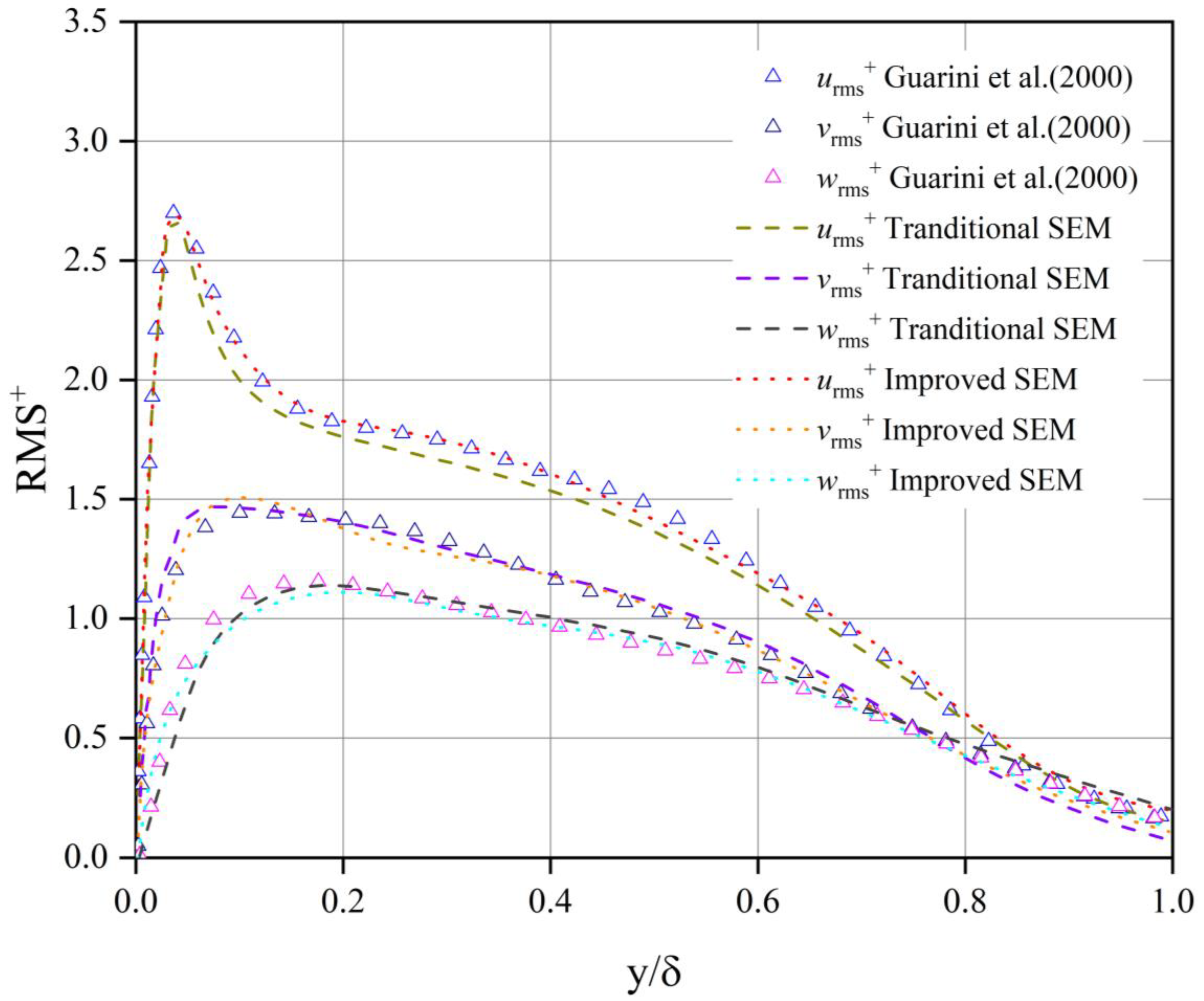
  1. Guarini, S.E.; Moser, R.D.; Shariff, K.; Wray, A. Direct numerical simulation of a supersonic turbulent boundary layer at Mach 2.5. J. Fluid Mech. 2000, 414, 1–33. [Google Scholar] [CrossRef] [Green Version]
  2. Dhamankar, N.S.; Blaisdell, G.A.; Lyrintzis, A.S. Overview of Turbulent Inflow Boundary Conditions for Large-Eddy Simulations. AIAA J. 2018, 56, 1317–1334. [Google Scholar] [CrossRef]
  3. Schlüter, J.U.; Pitsch, H.; Moin, P. Large-Eddy Simulation Inflow Conditions for Coupling with Reynolds-Averaged Flow Solvers. AIAA J. 2004, 42, 478–484. [Google Scholar] [CrossRef]
  4. Schlüter, J.U.; Wu, X.; Kim, S.; Shankaran, S.; Alonso, J.J.; Pitsch, H. A Framework for Coupling Reynolds-Averaged with Large-Eddy Simulations for Gas Turbine Applications. J. Fluids Eng. 2005, 127, 806–815. [Google Scholar] [CrossRef]
  5. Keating, A.; Piomelli, U.; Balaras, E.; Kaltenbach, H.-J. A priori and a posteriori tests of inflow conditions for large-eddy simulation. Phys. Fluids 2004, 16, 4696–4712. [Google Scholar] [CrossRef]
  6. Lund, T.S.; Wu, X.; Squires, K.D. Generation of Turbulent Inflow Data for Spatially-Developing Boundary Layer Simulations. J. Comput. Phys. 1998, 140, 233–258. [Google Scholar] [CrossRef] [Green Version]
  7. Mochida, A.; Lun, I.Y.F. Prediction of wind environment and thermal comfort at pedestrian level in urban area. J. Wind Eng. Ind. Aerodyn. 2008, 96, 1498–1527. [Google Scholar] [CrossRef]
  8. Uzun, A.; Hussaini, M.Y. Simulation of Noise Generation in the Near-Nozzle Region of a Chevron Nozzle Jet. AIAA J. 2009, 47, 1793–1810. [Google Scholar] [CrossRef]
  9. Wang, M.; Moin, P. Computation of Trailing-Edge Flow and Noise Using Large-Eddy Simulation. AIAA J. 2000, 38, 2201–2209. [Google Scholar] [CrossRef]
  10. Mathey, F.; Cokljat, D.; Bertoglio, J.P.; Sergent, E. Assessment of the vortex method for Large Eddy Simulation inlet conditions. Prog. Comput. Fluid Dyn. Int. J. 2006, 6, 58. [Google Scholar] [CrossRef]
  11. Xie, Z.-T.; Castro, I.P. Efficient Generation of Inflow Conditions for Large Eddy Simulation of Street-Scale Flows. Flow Turbul. Combust. 2008, 81, 449–470. [Google Scholar] [CrossRef] [Green Version]
  12. Jarrin, N.; Benhamadouche, S.; Laurence, D.; Prosser, R. A synthetic-eddy-method for generating inflow conditions for large-eddy simulations. Int. J. Heat Fluid Flow 2006, 27, 585–593. [Google Scholar] [CrossRef] [Green Version]
  13. Jarrin, N.; Prosser, R.; Uribe, J.C.; Benhamadouche, S.; Laurence, D. Reconstruction of turbulent fluctuations for hybrid RANS/LES simulations using a Synthetic-Eddy Method. Int. J. Heat Fluid Flow 2009, 30, 435–442. [Google Scholar] [CrossRef] [Green Version]
  14. Pamiès, M.; Weiss, P.-É.; Garnier, E.; Deck, S.; Sagaut, P. Generation of synthetic turbulent inflow data for large eddy simulation of spatially evolving wall-bounded flows. Phys. Fluids 2009, 21, 045103. [Google Scholar] [CrossRef]
  15. Poletto, R.; Craft, T.; Revell, A. A New Divergence Free Synthetic Eddy Method for the Reproduction of Inlet Flow Conditions for LES. Flow Turbul. Combust. 2013, 91, 519–539. [Google Scholar] [CrossRef]
  16. Tabor, G.R.; Baba-Ahmadi, M.H. Inlet conditions for large eddy simulation: A review. Comput. Fluids 2010, 39, 553–567. [Google Scholar] [CrossRef]
  17. Mankbadi, M.R.; DeBonis, J.R.; Georgiadis, N.J. Large-Eddy Simulation of a Compressible Mixing Layer and the Significance of Inflow Turbulence. In Proceedings of the 55th AIAA Aerospace Sciences Meeting, Grapevine, TX, USA, 9–13 January 2017; American Institute of Aeronautics and Astronautics: Reston, VA, USA, 2017. [Google Scholar]
  18. Lee, S.; Gross, A. Large-Eddy Simulation of Supersonic Turbulent Boundary Layer. In Proceedings of the AIAA AVIATION 2020 FORUM, Virtual Event, 15–19 June 2020; American Institute of Aeronautics and Astronautics: Reston, VA, USA, 2020. [Google Scholar]
  19. Lai, J.; Yu, H.; Tian, Z.; Li, H. Hybrid MPI and CUDA Parallelization for CFD Applications on Multi-GPU HPC Clusters. Sci. Program. 2020, 2020, 8862123. [Google Scholar] [CrossRef]
  20. Gjøsund, S.H. Simplified Approximate Expressions for the Boundary Layer Flow in Cylindrical Sections in Plankton Nets and Trawls. Open J. Mar. Sci. 2012, 2, 66–69. [Google Scholar] [CrossRef] [Green Version]
  21. Van Driest, E.R. Turbulent Boundary Layer in Compressible Fluids. J. Aeronaut. Sci. 1951, 18, 145–160. [Google Scholar] [CrossRef]
Figure 1. Eddy regeneration in traditional SEM.
Aerospace 09 00037 g001
Figure 2. Schematic diagram of the synthetic vortex region.
Aerospace 09 00037 g002
Figure 3. Movement of an eddy k in the synthetic eddy region.
Aerospace 09 00037 g003
Figure 4. Profiles of integral turbulence length scale and eddy radii.
Aerospace 09 00037 g004
Figure 5. Root mean square distributions of the velocity fluctuations within the boundary layer extracted from DNS results.
Aerospace 09 00037 g005
Figure 6. Schematic of the computational domain of a supersonic flat plate flow.
Aerospace 09 00037 g006
Figure 7. Streamwise pulsation velocity diagrams of the inlet turbulent boundary layer at different times.
Aerospace 09 00037 g007
Figure 8. Transient vorticity contours colored by density along the center section in the spanwise direction.
Aerospace 09 00037 g008
Figure 9. Instantaneous streamwise velocity contours and the second invariant Q contours (black line) of the velocity gradient tensor along the center section in the spanwise direction.
Aerospace 09 00037 g009
Figure 10. Isosurfaces of the second invariant Q colored by the streamwise velocity for the (a) traditional SEM and (b) improved SEM.
Aerospace 09 00037 g010aAerospace 09 00037 g010b
Figure 11. Mean velocity distributions at x = 12 δ .
Aerospace 09 00037 g011
Figure 12. Comparison of the computational C f with the experimental data: ×, simulation data point of simulation with improved SEM; ∗, simulation data point of DNS (Guarini et al., 2000); ○, experimental data points ( 2.2 M a 2.8 ) (Coles et al., 1954); solid line for Van Driest II (Bardina et al., 1997).
Aerospace 09 00037 g012
Figure 13. Comparison of the streamwise C f between the traditional SEM and the Improved SEM.
Aerospace 09 00037 g013
Figure 14. Root mean square velocity distribution at x = 12 δ for different methods.
Aerospace 09 00037 g014
Table 1. Computational grids for the mesh of the channel domain.
N x N y N z Total
(Million)
Δ x + Δ y + Δ z +
47336027045.988.2–13.21–124.1
Publisher’s Note: MDPI stays neutral with regard to jurisdictional claims in published maps and institutional affiliations.

