Unsteady Simulation of Transonic Buffet of a Supercritical Airfoil with Shock Control Bump

Abstract

The unsteady flow characteristics of a supercritical OAT15A airfoil with a shock control bump were numerically studied by a wall-modeled large eddy simulation. The numerical method was first validated by the buffet and nonbuffet cases of the baseline OAT15A airfoil. Both the pressure coefficient and velocity fluctuation coincided well with the experimental data. Then, four different shock control bumps were numerically tested. A bump of height h/c = 0.008 and location x_B/c = 0.55 demonstrated a good buffet control effect. The lift-to-drag ratio of the buffet case was increased by 5.9%, and the root mean square of the lift coefficient fluctuation was decreased by 67.6%. Detailed time-averaged flow quantities and instantaneous flow fields were analyzed to demonstrate the flow phenomenon of the shock control bumps. The results demonstrate that an appropriate “λ” shockwave pattern caused by the bump is important for the flow control effect.

1. Introduction

Modern civil aircraft usually adopt a supercritical wing and operate at transonic speed [1]. Shockwaves appear at both the cruise condition and the buffet condition for a supercritical wing or airfoil [2]. The buffet, which is a self-sustained shock oscillation induced by periodic interactions between a shockwave and a separated boundary layer [3], is a key constraint of the flight envelope of a civil aircraft [4].

The transonic buffet phenomenon has been studied for decades. It was first observed by Hilton and Fowler [5] in a wind tunnel investigation. When a buffet occurs, the shockwave location and the lift coefficient, as well as the turbulent boundary layer thickness after the shockwave, change periodically [5]. Iovnovich and Raveh [6] classified transonic buffets into two types: one is where a shock oscillation appears on both the upper side and lower side of the wing, while the other is where an oscillation only exists on the upper side. The latter is more common for a supercritical wing of a civil aircraft [7]. Pearcey et al. [8] studied the relation between the flow separation near the trailing edge and the onset of a buffet, which is widely used in the determination of the buffet onset boundary [3]. When the shockwave strength is weak, which is the case for a supercritical airfoil, the Kutta wave is believed to play an important role in the shockwave oscillation [9,10]. A self-sustained feedback model of a shockwave buffet was proposed by Lee et al. [10]. The model illustrated that when the pressure fluctuation of the shockwave propagates downstream of the trailing edge, the sudden change in the disturbance forms a Kutta wave propagating upstream, and the shockwave is made to oscillate by the energy contained in the Kutta wave [10]. The Kutta wave, which propagates by the speed of sound [10], is also considered a sound wave generated at the trailing edge [11]. Chen et al. [12] further extended the feedback model to more types of shockwave oscillations. Crouch et al. [13] found that both the stationary mode and oscillatory mode of instability occur on an unswept buffet wing, and that the intermediate-wavelength mode has a flow feature of the airfoil buffeting mode.

Experimental [14,15] and numerical investigations [16,17,18] have been widely used in buffet studies in recent years. The transonic buffet characteristics of an OAT15A supercritical airfoil were experimentally measured [14] and widely adopted as a validation case for numerical study. The unsteady Reynolds-averaged Navier–Stokes (RANS) method [16] and detached eddy simulation [17] can resolve the large-scale pattern of a transonic buffet and determine the main frequency of the shockwave oscillation, while a large eddy simulation (LES) [18] can provide abundant details of the interaction between the shockwave and turbulence structures inside the boundary layer.

The buffet onset boundary determines the flight envelope of a civil aircraft [19]. Suppressing the shockwave oscillation and improving the buffet onset lift coefficient are vital for modern civil aircraft design. Vortex generators [20] and shock control bumps (SCBs) [21] are two common passive flow control devices used for transonic buffets. The vortex generator has been intensively studied and widely adopted on Boeing’s civil aircraft to control the transonic buffet [22]. However, SCBs are still receiving considerable research attention and are not yet practical on civil aircraft. SCBs can be classified into two-dimensional (2D) bumps and three-dimensional (3D) bumps [23]. The 2D bump is identical along the spanwise direction, while the 3D bump can have different shapes in the spanwise direction.

The basic control mechanism of a 2D SCB is a combination of the compression wave and expansion wave near the shockwave [24]. A supercritical airfoil usually has a weak normal shock on the upper surface. If a bump is placed at the shockwave location, a compression wave can be formed when the flow moves upward from the bump and weakens the normal shock. Expansion waves downside of the bump are also beneficial for pressure recovery after the shockwave. With the compression and expansion waves, a “λ” shockwave structure is formed instead of a normal shock on the airfoil [25], meaning the wave drag can be reduced. As the benefit comes from the interaction between the shockwave and the bump, the drag reduction effect is relevant to the bump location and height. Sabater et al. [26] applied a robust optimization on the location and shape of a 2D SCB and achieved a drag reduction of more than 20% on an RAE2822 airfoil. Jia et al. [27] found that a 2D SCB can reduce the drag coefficient at a large lift coefficient; however, it increases the drag coefficient at a small lift coefficient. Adaptive SCBs [28,29], which change shapes according to the shockwave location, provide drag reduction effectiveness under a wide range of flow conditions. Lutz et al. [30] optimized adaptive SCBs and found the drag curve shows significant improvement compared to the initial airfoil.

The control mechanism of a 3D SCB includes not only the “λ” shockwave structure formed by the bump but also the vortical flow induced by the bump [31], which is similar to a small vortex generator [32]. The streamwise vortex induced by the edge of the 3D SCB is beneficial for the mixing of high-energy outer flow and low-energy boundary layer flow, consequently suppressing the flow separation. A 3D bump with a wedge shape [33,34] or hill shape [31,35,36] can effectively induce a vortical flow after the bump and change the shockwave behavior.

SCBs have shown great potential for buffet control. However, there are also some issues mentioned in the literature. One of the concerns is that the control efficiency is sensitive to the shock location [37]. This might decrease the performance at the off-design condition. An adaptive SCB can extend the effective range of shock control; however, an adaptive SCB might increase the structure complexity and maintenance cost [38].

From the numerical method perspective, the steady [39,40] or unsteady [32,41] RANS method has been widely used in the study of buffets or in the shape design of SCBs for supercritical airfoils. However, the control effect of SCBs is rarely studied by high-fidelity turbulence simulation methods such as the RANS–LES hybrid method or the LES method. As stated before, a buffet is a natural unsteady turbulent flow that includes periodic shockwaves and a thickened turbulent boundary layer under a high Reynolds number. A large eddy simulation can resolve the small-scale turbulent structures of the boundary and the generated acoustic waves of the tailing edge [18], which is a superior method to study the unsteady interaction mechanism between the shockwave and the SCB.

In this paper, the transonic buffet of an OAT15A supercritical airfoil with an SCB was numerically studied by a wall-modeled large eddy simulation (WMLES). The numerical method was validated by the experimental data of the OAT15A airfoil. Several 2D SCBs were adopted to test the control effect of the unsteady flow. The flow fields of both the nonbuffet case and buffet case were analyzed. To the authors’ knowledge, this is the first study to use a large eddy simulation on the SCB of a supercritical airfoil. The time-averaged flow quantities, periodic flow patterns and pressure fluctuations were compared for the airfoil without or with an SCB.

2. Numerical Method and Validation

2.1. Numerical Method

In this paper, a wall-modeled large eddy simulation was adopted to compute the flow field of an OAT15A supercritical airfoil. The solver was developed based on a finite-volume CFD code [42,43]. The inviscid flux was computed based on a blending of an upwind scheme and a central difference scheme [44,45]. The time advancing method is a three-step Runge–Kutta method. Vreman’s eddy viscosity model [46] was used to model the subgrid-scale turbulence motion. Based on the estimation of Choi and Moin [47], the grid requirement of a wall-resolving large eddy simulation is proportional to ${\mathrm{Re}}_L^{13/7}$, and L is the character length of the flow field; in contrast, the grid requirement of a wall-modeled simulation is proportional to ${\mathrm{Re}}_L$. In this study, the computational cost of a wall-resolving LES was too high because the Reynolds number is 3 × 10⁶. Consequently, an equilibrium stress-balanced equation was solved to model the energy-containing eddies in the inner turbulent boundary layer [44,45]. The wall-modeled equation was solved on an additional one-dimensional grid with 50 grid points to obtain the velocity profile of the inner layer of the boundary layer. The shear stress provided by the wall-modeled equation was applied as the boundary condition of the Navier–Stokes equation. The velocity of the upper boundary of the wall-modeled equation was interpolated from the third layer of the LES grid. The numerical method is not the focus of this paper. Consequently, detailed numerical schemes and formulas are not presented here. Readers can refer to our previous work on high-Reynolds separated flows [44,45].

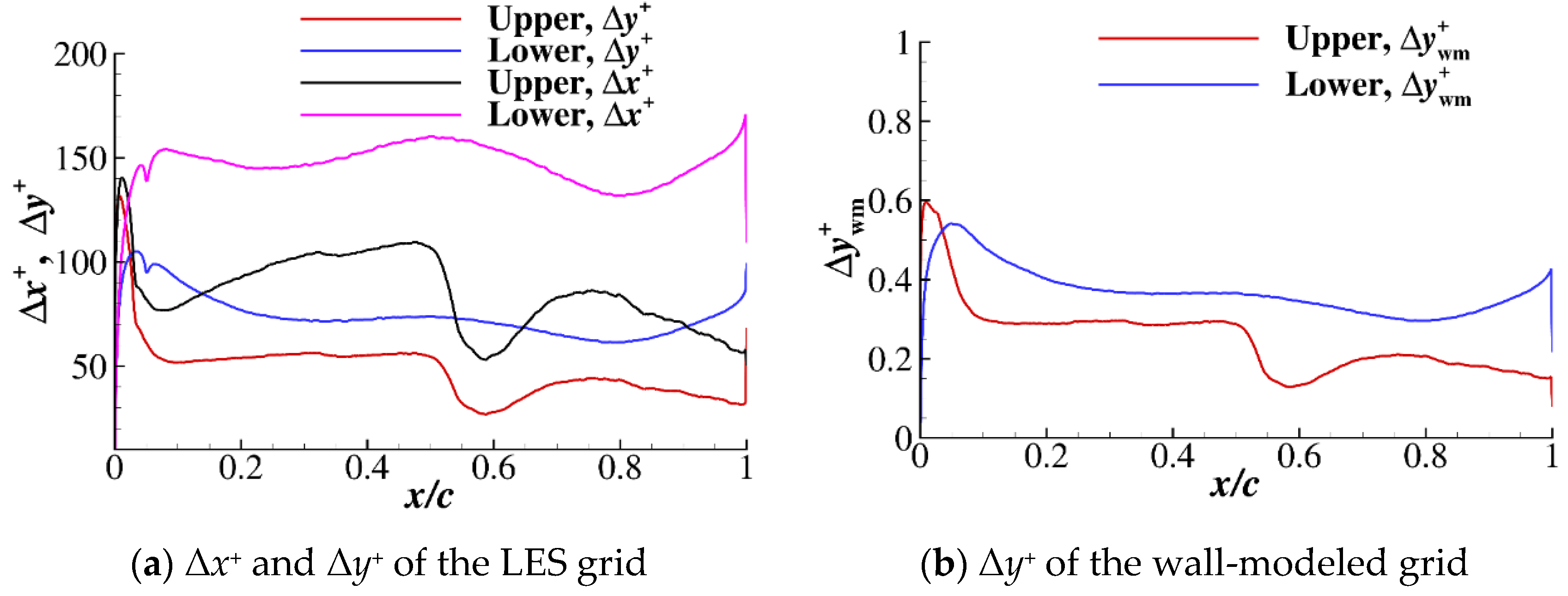
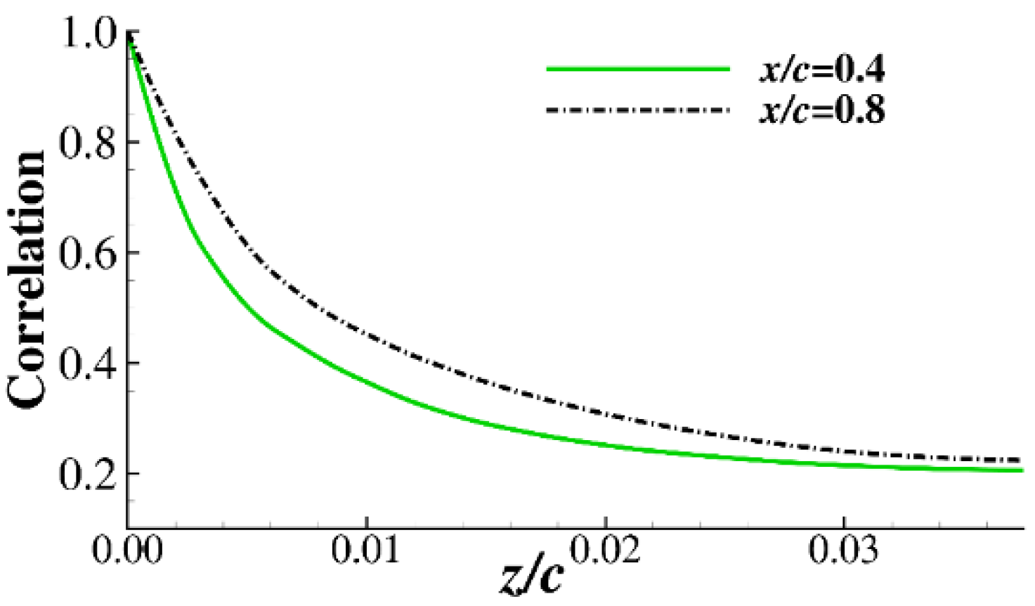
2.2. Computational Grid

The computational grid used in this paper was a C-type grid, which was generated by an in-house grid generation code that solves Poisson’s equation. The computational domain was [−18c, 20c] in the x direction and [−20c to 20c] in the y direction (c is the chord length). Although the bump shape was two-dimensional, we carried out a three-dimensional simulation because of the three-dimensional nature of the turbulence. The spanwise length was 0.075c, which is larger than the WMLES in the study by Fukushima et al. [18]. The grid had 1945 points in the circumferential direction and 261 points in the normal direction. It had 51 points evenly located in the spanwise direction. The trailing edge thickness was 0.005c, and a grid block with 21 × 51 × 249 points was located on the trailing edge region. The total grid number was 26.2 million. Figure 1a shows the grid of the x–y plane of the baseline OAT15A airfoil. The figure is plotted by every two points of the grid. Figure 1b shows the wall grid near the leading edge of the airfoil. The first layer height of the grid was 2.0 × 10⁻⁴c. The increasing ratio in the normal direction was less than 1.1. The first grid layer can be located in the logarithmic layer of the turbulent boundary layer because the wall-modeled equation can provide the shear stress boundary condition of the wall. When the SCB was installed on the airfoil surface, the wall surface was deformed to simulate the effect of the bump while keeping the grid topology and grid number the same.

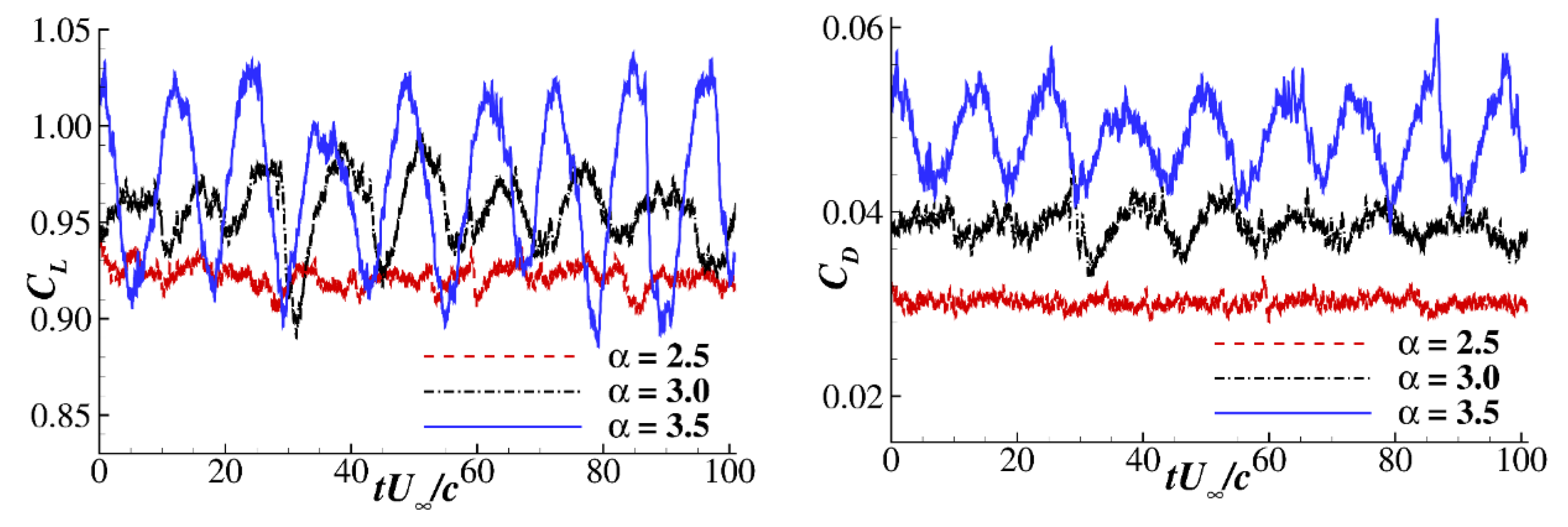
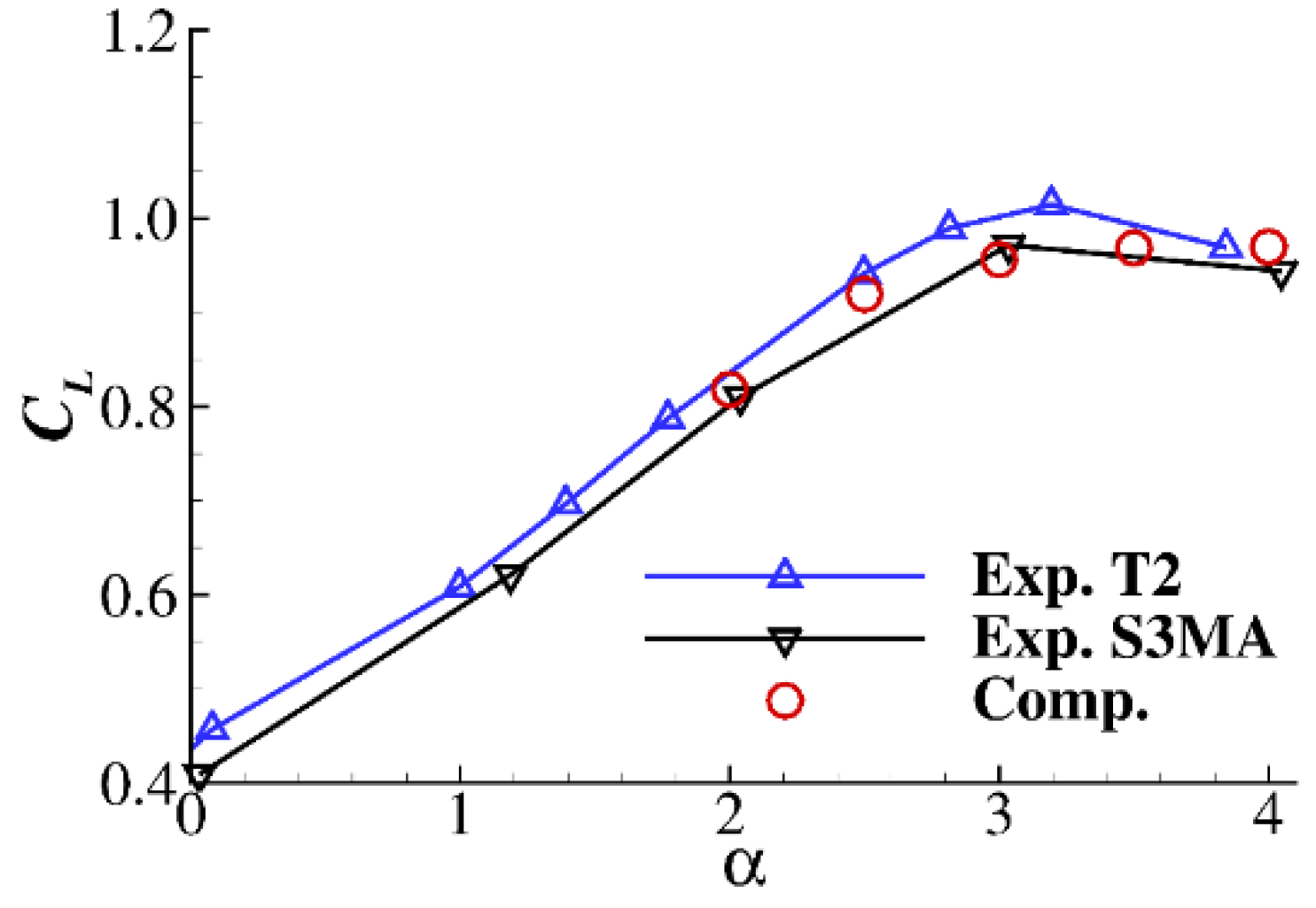
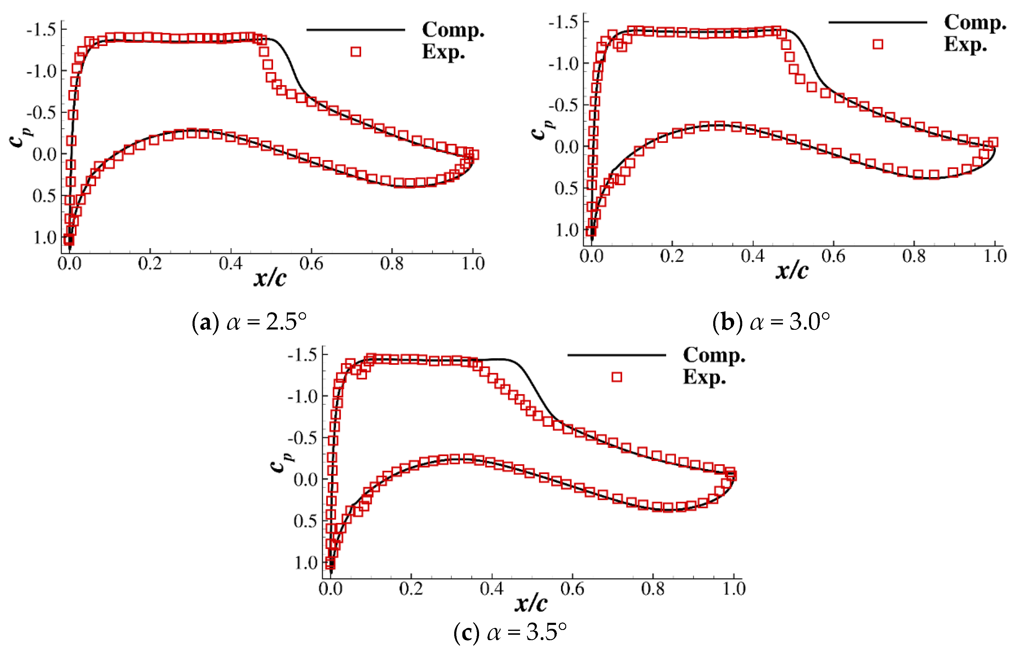
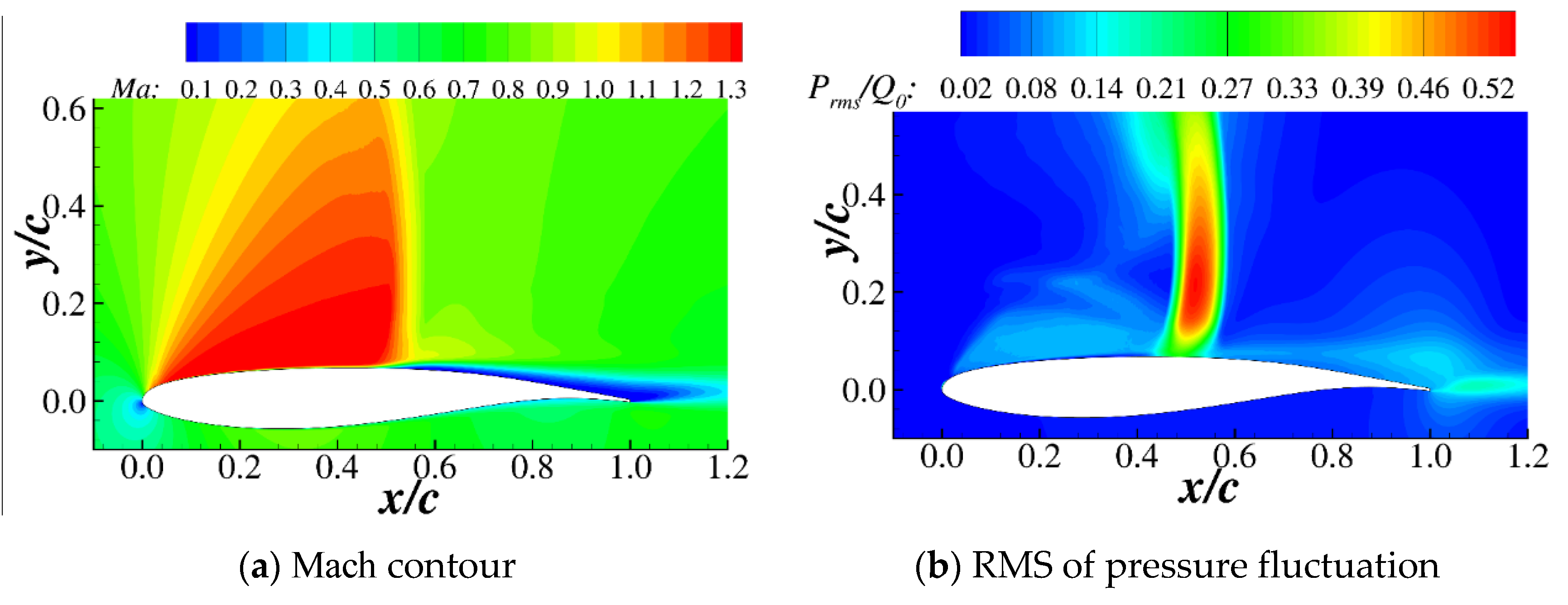
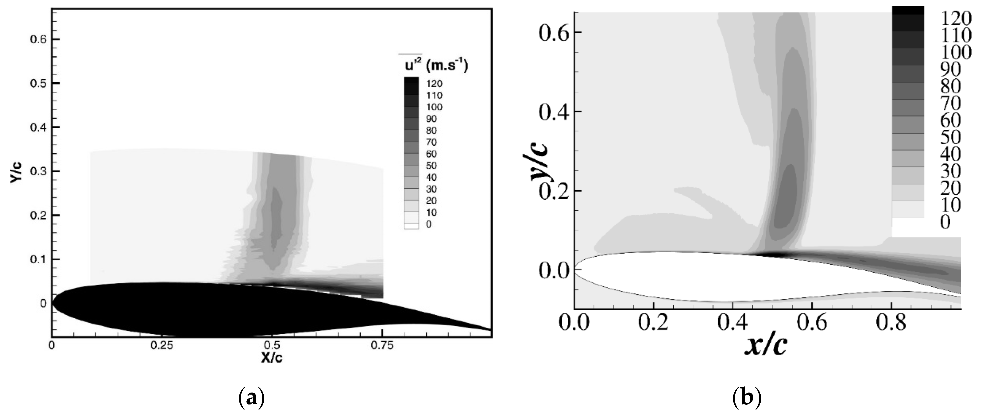
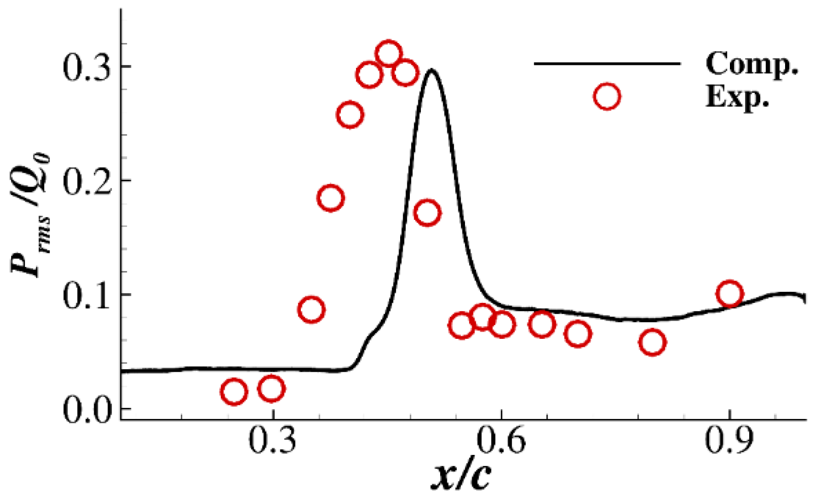
2.3. Validation of the Baseline OAT15A Airfoil

The baseline OAT15A airfoil was adopted as the validation case. The flow condition was Ma = 0.73 and Re = 3.0 × 10⁶. [14] The nondimensional time step was ΔtU_∞/c = 1.37 × 10⁻⁴. Approximately 180 time units (tU_∞/c) were computed for each case, and the last 100 time units were applied for flow field statistics. It cost approximately 2.0 × 10⁵ core hours for each flow case on an Intel cluster with a 2.0 GHz CPU.

The Δx⁺ and Δy⁺ of the first grid layer were collected to demonstrate the grid resolution of the present computation. Figure 2a shows the Δx⁺ and Δy⁺ of the LES grid collected by an angle of attack α = 2.5°. Δy⁺ was approximately 50 on the upper surface and 80 on the lower surface, while Δx⁺ was approximately twice the Δy⁺. The first grid point in the wall normal direction was located at the logarithmic layer of a turbulent boundary layer, which satisfies the requirement for a WMLES. The Δy⁺ of the first grid layer of the wall-modeled equation (Δy⁺_wm) was always less than 1.0, as shown in Figure 2b. This is sufficient to describe the viscous sublayer of the turbulent boundary layer. The spanwise correlation [43] of the pressure fluctuation was computed to test the spanwise domain. As shown in Figure 3, the correlations of both x/c = 0.4 and 0.8 damp fast in the spanwise direction, which demonstrates that the present spanwise domain size (0.075 c) is adequate.

Figure 4 shows the lift and drag coefficient histories at three different angles of attack. When a buffet does not occur (α = 2.5°), the lift and drag coefficients have oscillations with small amplitudes. Then, the amplitude of oscillation is increased at α = 3.0°. When α = 3.5°, a clear periodic oscillation pattern appears on both the lift and drag coefficients, which demonstrates that a buffet occurs.

The lift coefficient was time-averaged for comparison with the experimental data, as shown in Figure 5. The experimental data were extracted from [48]. There were two series of experimental data in the reference. One was from the S3MA wind tunnel, and the other was from the T2 wind tunnel. The Reynolds number in that experiment was 6.0 × 10⁶, which is higher than the present computation. Although the flow condition was slightly different from the present computation, the time-averaged lift coefficients of the present computation were located between the two series of experimental data.

The mean pressure coefficient was compared with the experimental data of [14]. As shown in Figure 6, the pressure coefficients at three different angles of attack coincide well with the experimental data, except that the shockwave location is slightly downstream of the experimental data.

Figure 7a shows the mean Mach contour at α = 3.5°. It is clear that a low-speed region appears near the trailing edge of the airfoil. The mean shockwave is also smeared because of the periodic oscillation of the shock location. Figure 7b demonstrates the root mean square (RMS) of the pressure fluctuations. It is normalized by the dynamic pressure of the freestream condition. The maximum pressure fluctuation appears near the shockwave location. Figure 8 compares the RMS of the streamwise velocity fluctuation with the experimental data of the S3Ch wind tunnel [49]. The values in Figure 8 are dimensional, and the contours have the same legend. The contours of the computation and experiment are quite consistent in both shape and value, which validates that the present computational method is reliable.

Figure 9 further compares the wall pressure fluctuation at α = 3.5°. The experimental data were extracted from [14]. The computed location of the peak fluctuation is slightly downstream, which is consistent with the pressure coefficient distribution (Figure 6c). However, the peak value of the present computation is close to the experiment, which means that the primary shock buffet phenomenon is well captured by the computation. The motivation of the present paper was to study the effect of the shock control bump. The variation caused by the bump, rather than the accurate shockwave location, is our focus in the following sections. Consequently, the numerical method is validated to be practicable.

3. Numerical Study of Shock Control Bump

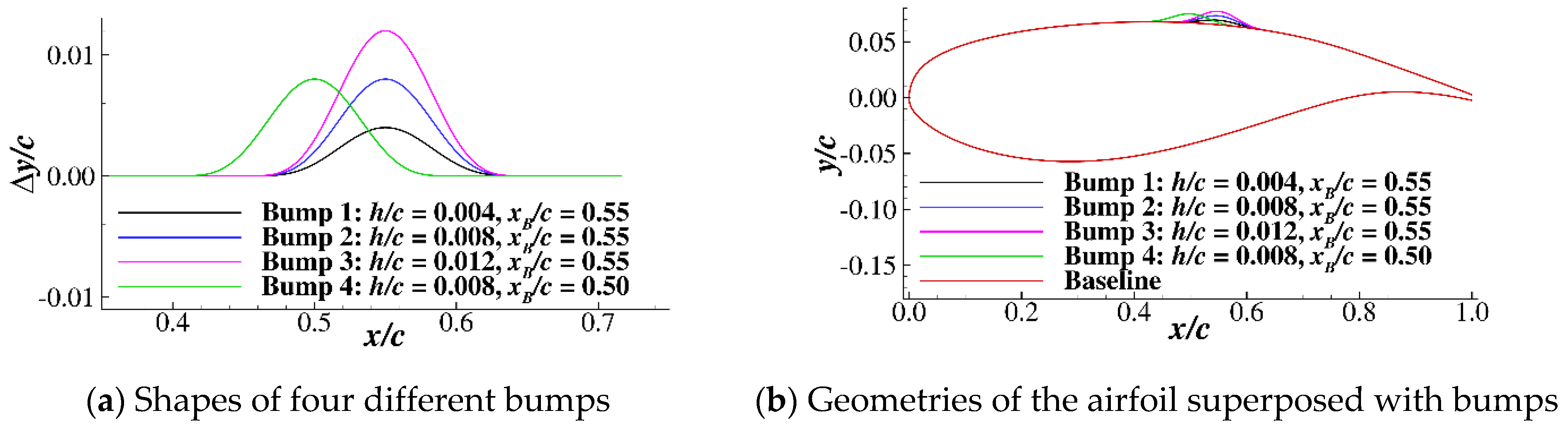
3.1. Shape of the Shock Control Bump

In this section, a two-dimensional SCB is numerically tested and compared with the baseline configuration. Several bumps with different heights and locations are analyzed. The geometries of the bumps are controlled by the Hicks–Henne function [27], as shown in Equation (1). The bump function f(x_B) is superposed on the baseline airfoil. h/c is the relative height of the bump, x_B/c is the central location and l_B is the bump length. Figure 10 shows the geometries of bumps with different parameters. Four bumps are computed in this paper, as shown in Figure 10a. The lengths of the bumps are 0.2c. The first three bumps are all located at x_B/c = 0.55, which is the shockwave location of the baseline OAT15A airfoil. The relative heights h/c of the first three bumps are 0.004, 0.008 and 0.012. The fourth bump is located slightly upstream x_B/c = 0.50 and has the same height as Bump 2. Figure 10b shows the geometries of the airfoil superposed with the bumps.

$$f(x_B)=\frac{h}{c}\cdot {\sin }^4\left[\frac{\pi (x/c-x_B/c)}{l_B}+\frac{\pi }{2}\right],x_B/c-l_B/2\le x/c\le x_B/c+l_B/2$$

(1)

The computational settings are the same as the baseline OAT15A airfoil in Section 2. The computational grids of the bump configurations are deformed from the baseline grid, which keeps the computation appropriate to compare with the baseline OAT15A airfoil.

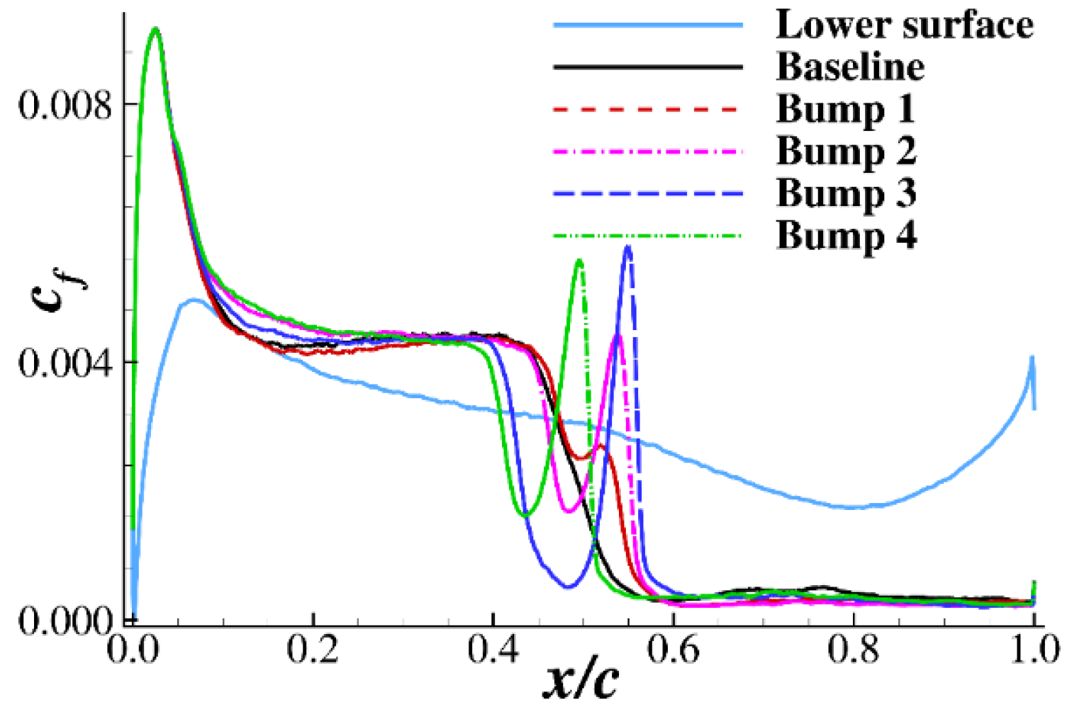
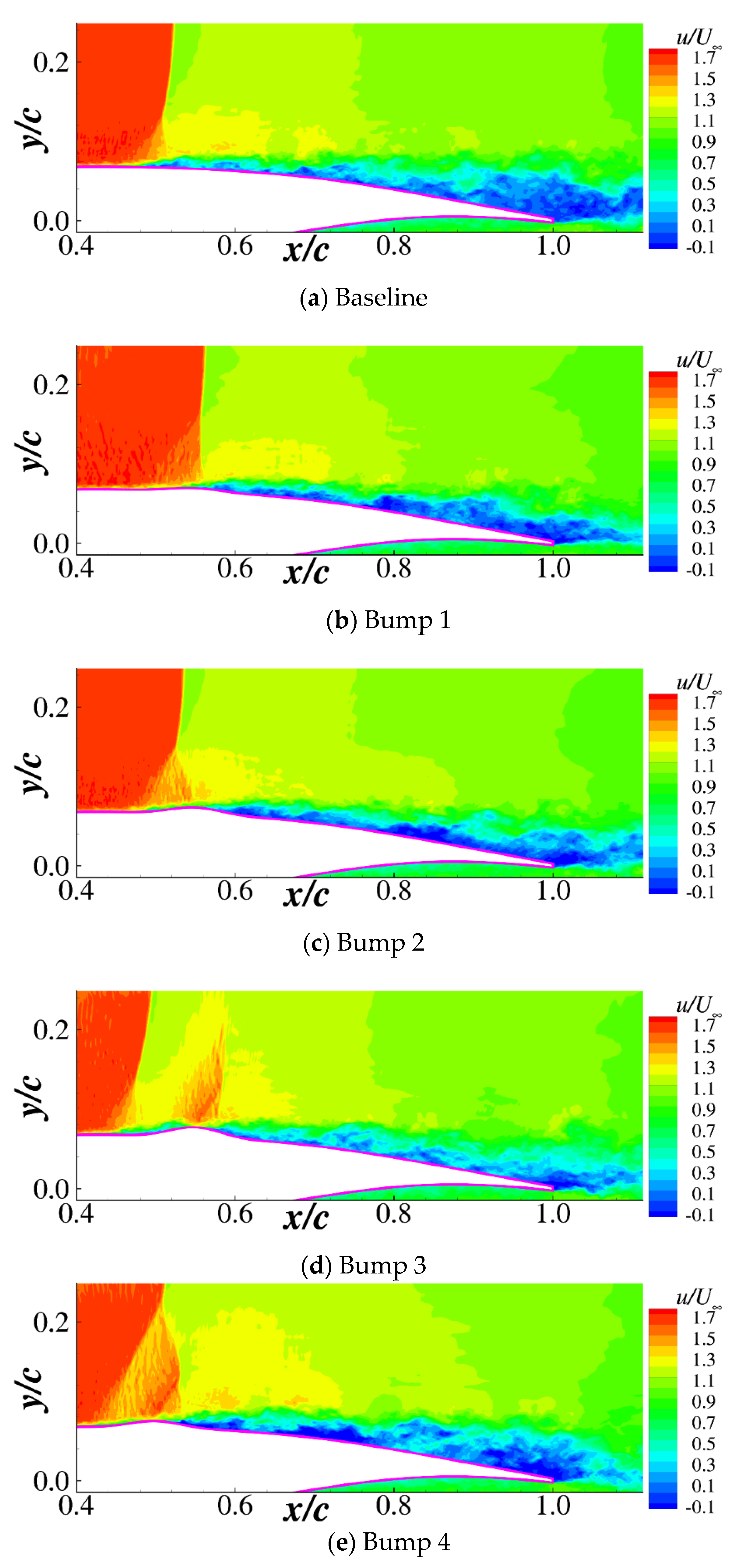
3.2. Time-Averaged Characteristics of the Airfoil with Bumps

The aerodynamic performance of the airfoil with bumps was computed and compared with the baseline airfoil. The nondimensional time step is ΔtU_∞/c = 1.37 × 10⁻⁴. The flow field of the baseline airfoil is used as the initial condition of the bump cases. More than 130 time units (tU_∞/c) are computed for each case. The last 80 time units are used for time averaging to obtain the aerodynamic coefficients. Six cases were computed, which are α = 3.5° for all four bumps and α = 2.5° for Bump 2 and Bump 4.

Figure 11 shows the histories of the lift and drag coefficients in the computation. It is obvious that the periodic oscillation of the lift and drag coefficients at α = 3.5° is suppressed by Bumps 2, 3 and 4, while Bump 1 has very little effect on the lift oscillation. It can be seen that the bumps may have a negative influence on the lift coefficient. The lift coefficient is more or less decreased at α = 3.5°, while it is significantly decreased at the nonbuffet condition α = 2.5°. Moreover, the drag coefficient is also influenced by the bumps. The drag coefficient at α = 2.5° is notably increased, as shown in Figure 11d.

The time-averaged values of the aerodynamic coefficients are listed in

Table 1. Time-averaged aerodynamic coefficients of the airfoil with bumps.

Configuration	Angle of Attack	Lift Coefficient	RMS of Lift Coefficient	Drag Coefficient	RMS of Drag Coefficient	Lift-to-Drag Ratio	Pitching Moment
Baseline airfoil	2.5°	0.919	0.006884	0.03009	0.000724	30.54	−0.1335
	3.5°	0.968	0.037572	0.04823	0.003737	20.07	−0.1262
Bump 1 (h/c = 0.004, xB/c = 0.55)	3.5°	0.965 (−0.3%)	0.027828 (−25.9%)	0.04634 (−3.9%)	0.003107 (−16.8%)	20.82 (+3.7%)	−0.1252 (+0.8%)
Bump 2 (h/c = 0.008, xB/c = 0.55)	2.5°	0.866 (−5.8%)	0.004527 (−34.2%)	0.03174 (+5.5%)	0.000662 (−8.6%)	27.28 (−10.6%)	−0.1260 (+5.6%)
	3.5°	0.953 (−1.5%)	0.012188 (−67.6%)	0.04484 (−7.0%)	0.001569 (−58.0%)	21.25 (+5.9%)	−0.1229 (+2.6%)
Bump 3 (h/c = 0.012, xB/c = 0.55)	3.5°	0.917 (−5.3%)	0.008297 (−77.9%)	0.04642 (−3.8%)	0.001343 (−64.1%)	19.75 (−1.6%)	−0.1184 (+6.2%)
Bump 4 (h/c = 0.008, xB/c = 0.50)	2.5°	0.870 (−5.3%)	0.003852 (−44.0%)	0.03395 (+12.8%)	0.000549 (−24.2%)	25.63 (−16.1%)	−0.1271 (+4.8%)
	3.5°	0.925 (−4.4%)	0.016171 (−56.9%)	0.04559 (−5.5%)	0.002168 (−42.0%)	20.29 (+1.1%)	−0.1193 (+5.5%)

. The relative variations (in percentage) in the coefficients compared with the baseline configuration are also listed in the parentheses of the table. A tendency of the bumps is that the lift coefficient is consistently decreased by the four bumps at both α = 2.5° and α = 3.5°. The lift coefficient at α = 2.5° is decreased by approximately 5%, and it is decreased by approximately 1% to 5% at α = 3.5°. With increasing bump height (Bumps 1, 2 and 3), the lift drop becomes increasingly significant. If the location of the bump is moved upstream (Bumps 2 and 4), the lift decrement caused by the bump becomes larger. The influence of the bump on the drag coefficient is distinctly different under the nonbuffet and buffet conditions. The drag coefficient is increased at α = 2.5°, and it is reduced at α = 3.5°. Consequently, the lift-to-drag ratio is increased at the buffet case α = 3.5°, except for the highest bump (Bump 3), while the lift-to-drag ratio is decreased at the nonbuffet case α = 2.5°. Consequently, the bump is beneficial for the buffet case and might be harmful for the nonbuffet case, which coincides with our previous study based on Reynolds-averaged Navier–Stokes computation [27]. The pitching moment is also listed in the table. The reference points of the moment are x/c = 0.25 and y = 0. The negative value means a nose-down moment. It can be seen that the absolute values of the moment are all decreased by the SCBs; however, the variations are not significant.

A more interesting phenomenon shown in Table 1 is that regardless of whether the lift and drag are increased or decreased, the RMSs of the coefficients are all suppressed by the bumps. With increasing bump height, the suppression effect of the lift oscillation is more significant. In the present computation, Bump 2 has the highest increment of L/D α = 3.5° and a good suppression effect on the shockwave oscillation. The L/D of the buffet case is increased by 5.9%, and the RMS of the lift coefficient fluctuation is decreased by 67.6%; consequently, it is considered a good SCB design, with an appropriate height and location.

Figure 12 shows the time-averaged Mach contour of the four bumps. Bump 1 has the lowest height, meaning the shock pattern is similar to the baseline configuration in Figure 7a. A clear “λ”-type shock is formed near the shockwave foot of Bump 2 and Bump 4. However, the “λ” shock of Bump 4 is stronger than that of Bump 2, which results in more lift loss and less drag reduction. Bump 3 has the highest bump height. As shown in Figure 12c, the bump pushes the first shock upstream and forms a second shock on the bump; consequently, the aerodynamic performance of this bump is worse than the others.

Figure 13 presents the pressure coefficients of the airfoil with bumps. For the drag reduction cases (α = 3.5°), the strong shockwave of the baseline configuration is divided into two weak shockwaves. In contrast, for the drag increment cases (α = 2.5°), the shockwave is also divided, but the strength of the second shockwave is even stronger than that of the baseline airfoil.

Figure 14 shows the time-averaged wall friction coefficient of the airfoil. It is worth noting that the wall friction is computed by the wall-modeled equation. The lower surface is hardly influenced by the upper surface bumps, meaning only the lower surface c_f of the baseline airfoil is plotted in the figure. The wall friction coefficient of the upper surface is strongly affected by the bumps. The friction first declines when approaching the bump and then increases on the bump, which coincides with the tendency of the flow acceleration on the bump (Figure 12).

Figure 15 presents the velocity profile and Reynolds stresses inside the shockwave/boundary layer-induced flow separation region. Two locations at x/c = 0.6 and 0.8 are presented. The velocity near the bump (x/c = 0.6) is decreased by the bumps, as shown in Figure 15a, while the velocity profile becomes plump at x/c = 0.8 for Bumps 1 and 2. The RMS of the streamwise velocity fluctuation is equivalent to the square root of the Reynolds normal stress <u’u’>. The Reynolds shear stress is relevant to the wall friction. The Reynolds normal stresses are all suppressed by all bumps, while the shear stress is increased by Bumps 3 and 4 at x/c = 0.6. Bump 2 has the best Reynolds stress suppression effect on both normal stress and shear stress at both locations.

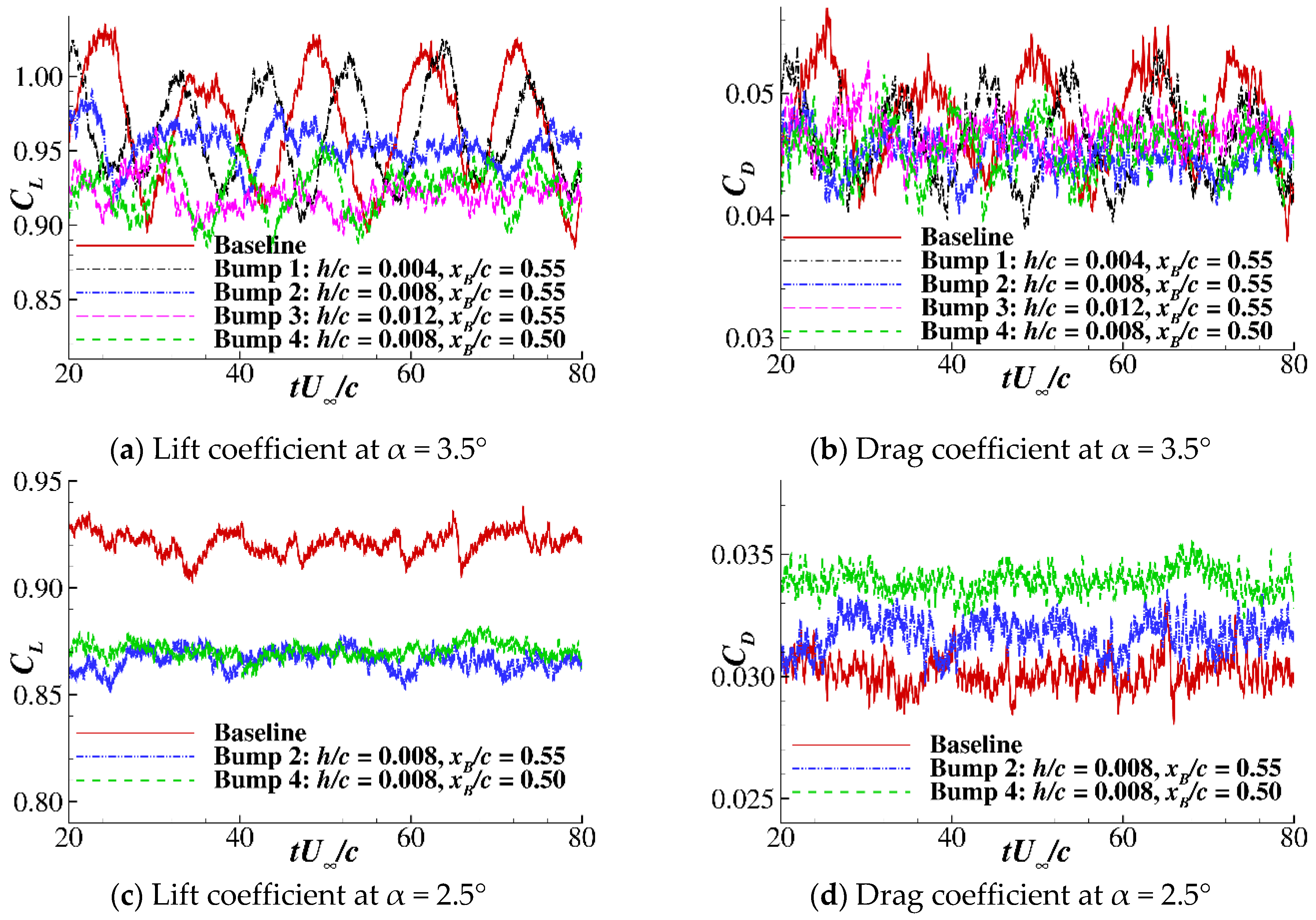
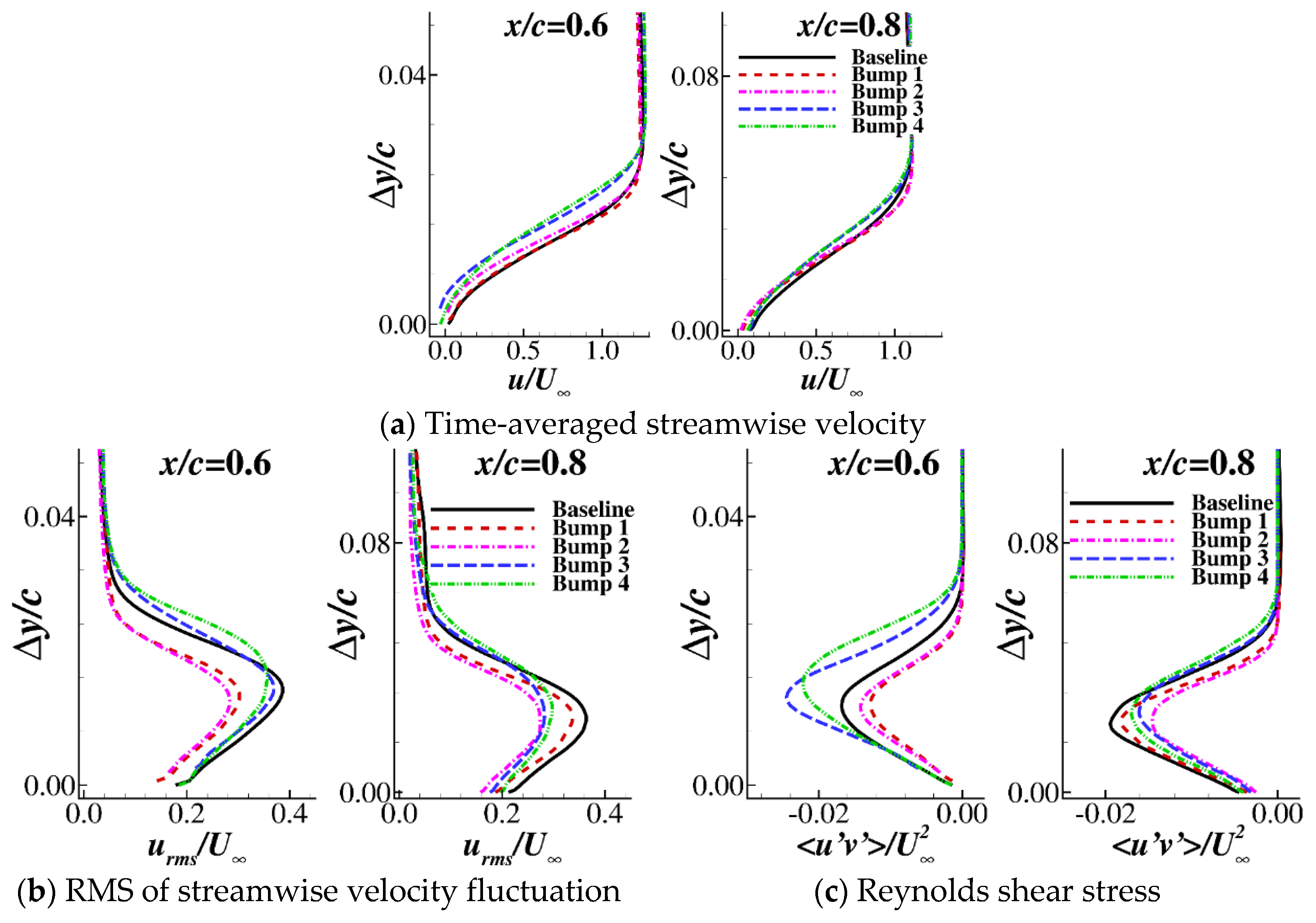
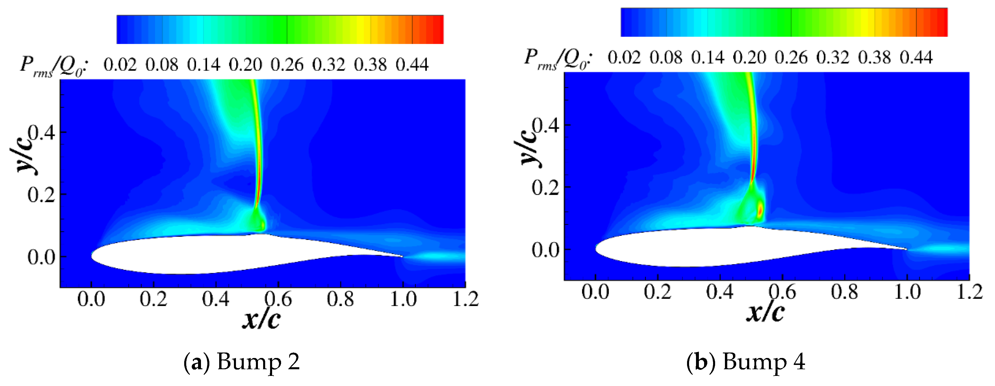
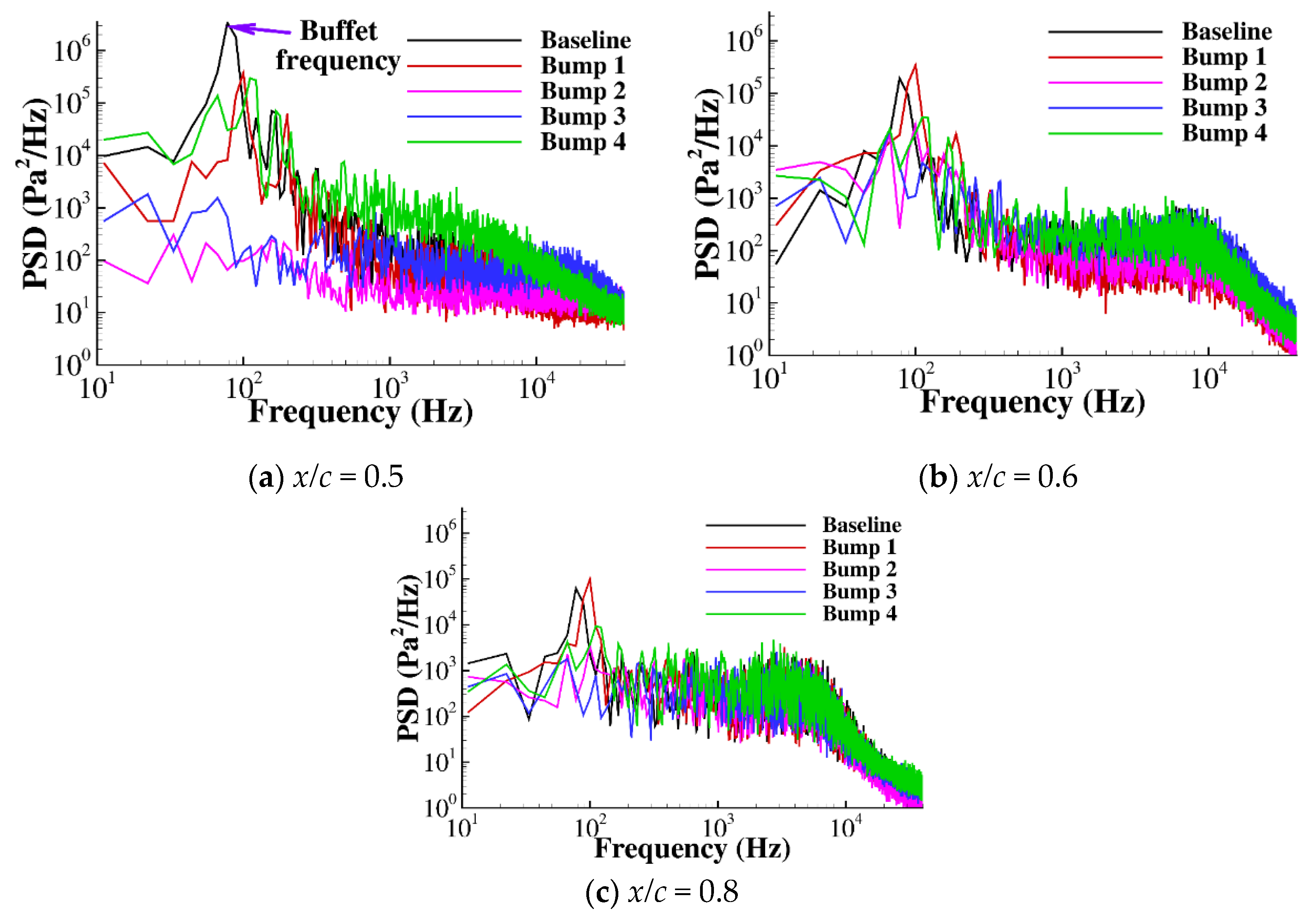
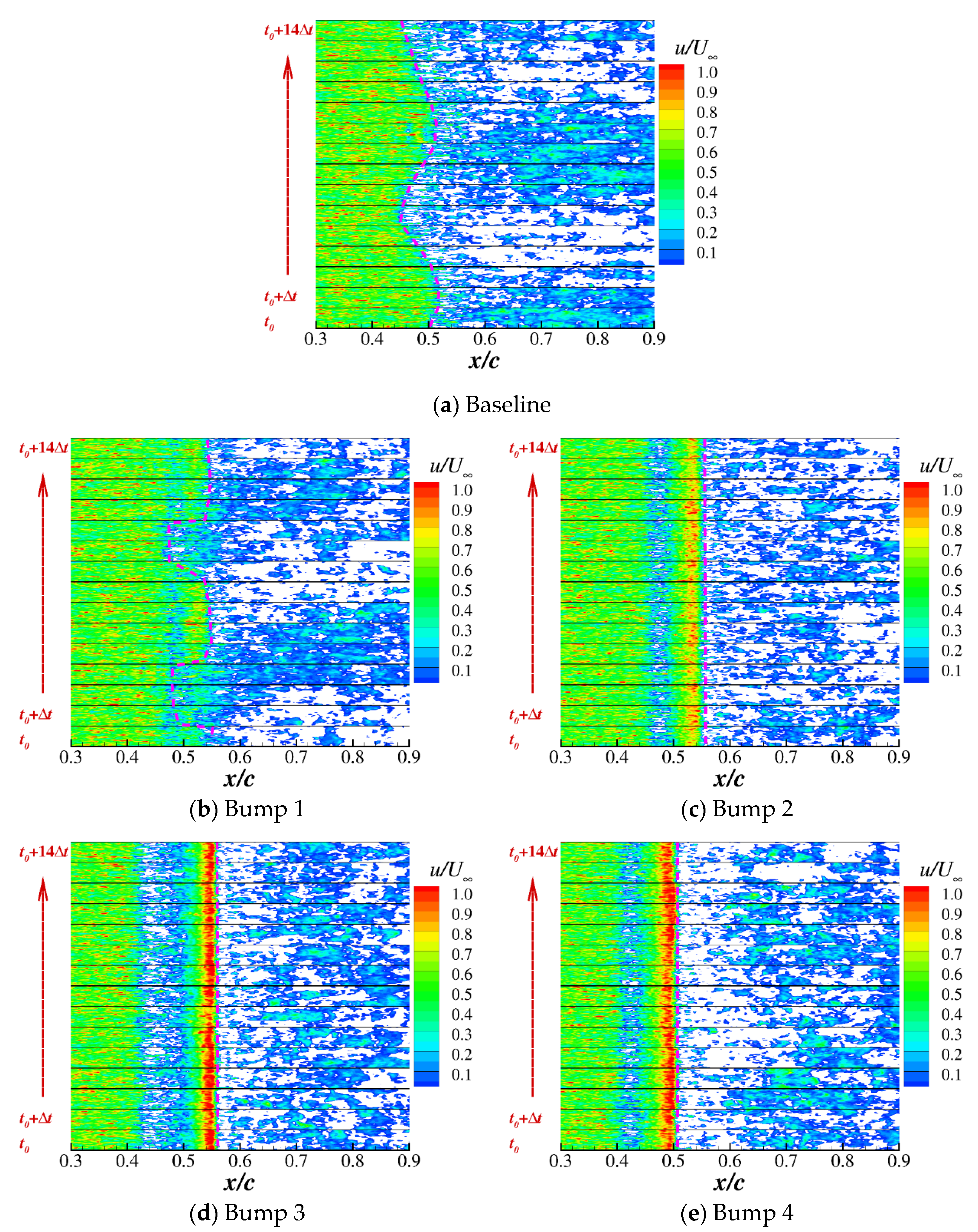
3.3. Fluctuation Characteristics of the Airfoil with Bumps

The fluctuations of the baseline airfoil and airfoil with SCBs are compared in this section. The RMS of the pressure fluctuation on the upper surface is shown in Figure 16. It is clear that the pressure fluctuation of the baseline airfoil is significantly suppressed by the bumps. Bump 2 has the smallest RMS value of the pressure fluctuation among the five cases, which is coincident with the fluctuation of the lift and drag coefficients. Not only the fluctuation near the shockwave but also the fluctuation near the trailing edge is suppressed by Bump 2. Bump 3 and Bump 4 also have favorable suppression effects on the pressure fluctuation.

Figure 17 shows the RMS contours of the pressure fluctuations for Bump 2 and Bump 4. It is clear that the high-fluctuation region near the shockwave is decreased when compared with the baseline configuration (Figure 7b). The “λ” shock region has a high pressure fluctuation, while the shockwave above the “λ” shock is quite stable. It is interesting that the shockwave far away from the airfoil fluctuates greatly. This demonstrates that the expansion wave forms near the leading edge region, weakening the strength of the shockwave and inducing unsteadiness, which is a basic principle of the design of a supercritical airfoil [50].

Three streamwise locations on the airfoil are sampled to compare the power spectral density (PSD) of the pressure fluctuation, as shown in Figure 18. The locations x/c = 0.5 and 0.6 are near the shockwave, and x/c = 0.8 is located in the low-speed region near the trailing edge. The dimensional quantities in Figure 18 are scaled based on the length of the experiment [14]. It is clear that a peak frequency appears on the baseline airfoil, which is the buffet frequency of the baseline airfoil. With the SCBs, the PSD of the pressure fluctuation is significantly reduced at x/c = 0.5. The buffet frequency of the baseline configuration is clear even at the downstream x/c = 0.8. Bump 1 has the lowest height, meaning the buffet is slightly suppressed by Bump 1, and the buffet frequency is slightly increased. Bump 2 is the most effective SCB because there is almost no frequency peak for the Bump 2 configuration.

Figure 19 shows the streamwise velocity contours of the first grid layers of the baseline airfoil and airfoil with bumps. As the present computation adopted a wall-modeled simulation, the grid spacing of the first grid layer is located at Δy+ of approximately 50, as shown in Figure 2a; consequently, the first grid layer of the LES has a considerably large flow speed. The white regions in the contours of Figure 19 are blanked when u < 0.0. Fifteen instantaneous snapshots with Δt = 1.37c/U_∞ are plotted along the vertical direction in each figure. It is clear that the high-speed region of the baseline airfoil (Figure 19a) oscillates periodically. When Bump 1 is installed on the upper surface (Figure 19b), the oscillation is weakened, but periodical oscillation still exists. The high-speed regions of Bumps 2, 3 and 4 are almost constant over time. However, strong flow acceleration regions appear at the bump locations of Bumps 3 and 4. Moreover, an instantaneous reverse flow (u < 0.0) can be seen before Bumps 3 and 4 at 0.4 < x/c < 0.5, which means that an inappropriate set of SCBs may induce an unexpectedly low-speed region before the bump. Although Bump 2 has a good control effect for the shock oscillation, an instantaneous reverse flow (u < 0.0) region also exists after the bump, which coincides with the mean flow contour shown in Figure 12b.

Figure 20 shows the instantaneous streamwise velocity contours of the airfoils. The unsteady flow separation near the trailing edge is strong for the baseline airfoil. With bump installation, trailing edge separation is suppressed. A “λ”-type shockwave can be seen near Bump 2. A secondary shockwave is formed for Bumps 3 and 4.

Figure 21 shows the instantaneous density fluctuations ($\mathsf{\Delta }\rho =\rho -{\rho }_{AVG}$) of the baseline airfoil and Bump 2 configuration. The sound wave propagates from the trailing edge, which is called the Kutta wave and is clear on the lower side of the airfoil. It is not so clear on the upper side because the flow phenomenon is complex, and many different waves (shockwave, expansion wave, sound wave, etc.) are mixed together. It can be seen from the lower side that the amplitude of the Kutta wave is weakened by the bump, and the characteristic wavelength is also changed; consequently, the buffet strength of the airfoil is weakened, which confirms the buffet mechanism explained by Lee et al. [10].

4. Conclusions

This paper adopted a wall-modeled large eddy simulation method to analyze the buffet control effect of a shockwave control bump. This work can be summarized as follows:

(1) The numerical method was validated by the baseline OAT15A airfoil. With the present wall-modeled equation, the grid requirement of the LES near the wall was greatly reduced. The pressure coefficient and RMS of the velocity fluctuation matched well with the experiment, which validates the reliability of the present computation.

(2) Four different two-dimensional bumps were numerically tested and analyzed. The time-averaged aerodynamic coefficients showed that the SCB was beneficial for the lift-to-drag ratio of the buffet condition but decreased the lift-to-drag ratio of the nonbuffet case. The fluctuations of the lift and drag coefficients can be greatly suppressed by the bumps. An appropriate “λ” shockwave pattern is important for the control effect of the SCB.

(3) The instantaneous flow characteristics of the airfoil with bumps were compared. The power spectral density of the pressure fluctuation demonstrated that the buffet frequency is almost eliminated by an appropriate bump. The instantaneous flow fields and Kutta wave explain the flow control mechanism of the SCB.

References

1. Niu, W.; Zhang, Y.; Chen, H.; Zhang, M. Numerical study of a supercritical airfoil/wing with variable-camber technology. Chin. J. Aeronaut. 2020, 33, 1850–1866. [Google Scholar] [CrossRef]
2. Li, R.; Deng, K.; Zhang, Y.; Chen, H. Pressure distribution guided supercritical wing optimization. Chin. J. Aeronaut. 2018, 31, 1842–1854. [Google Scholar] [CrossRef]
3. Lee, B.H.K. Self-sustained shock oscillations on airfoils at transonic speeds. Prog. Aerosp. Sci. 2001, 37, 147–196. [Google Scholar] [CrossRef]
4. Kenway, G.K.W.; Martins, J.R.R.A. Buffet-onset constraint formulation for aerodynamic shape optimization. AIAA J. 2017, 55, 1930–1947. [Google Scholar] [CrossRef]
5. Hilton, W.F.; Fowler, R.G. Photographs of Shock Wave Movement, NPL R &M No. 2692; National Physical Laboratories: Teddington, UK, 1947. [Google Scholar]
6. Iovnovich, M.; Raveh, D.E. Reynolds-averaged Navier-stokes Study of the Shock-buffet Instability Mechanism. AIAA J. 2012, 50, 880–890. [Google Scholar] [CrossRef]
7. Zhang, W.; Gao, C.; Ye, Z. Research Advances on Wing/Airfoil Transonic Buffet. Acta Aeronaut. Astronaut. Sin. 2015, 36, 1056–1075. (In Chinese) [Google Scholar]
8. Pearcey, H.H.; Osborne, J.; Haines, A.B. The Interaction Between Local Effects at the Shock and Rear Separation—A Source of Significant Scale Effects in Wind-Tunnel Tests on Aerofoils and Wings, AGARD CP-35; Transonic Aerodynamics: Paris, France, 1968; pp. 1–23. [Google Scholar]
9. Tijdeman, H.; Seebass, R. Transonic flow past oscillating airfoils. Annu. Rev. Fluid Mech. 1980, 12, 181–222. [Google Scholar] [CrossRef]
10. Lee, B.H.K.; Murty, H.; Jiang, H. Role of Kutta waves on oscillatory shock motion on an airfoil. AIAA J. 1994, 32, 789–796. [Google Scholar] [CrossRef]
11. Hartmann, A.; Feldhusen, A.; Schröder, W. On the interaction of shock waves and sound waves in transonic buffet flow. Phys. Fluids 2013, 25, 026101. [Google Scholar] [CrossRef]
12. Chen, L.; Xu, C.; Lu, X. Numerical investigation of the compressible flow past an aerofoil. J. Fluid Mech. 2009, 643, 97–126. [Google Scholar] [CrossRef] [Green Version]
13. Crouch, J.D.; Garbaruk, A.; Strelets, M. Global instability in the onset of transonic-wing buffet. J. Fluid Mech. 2019, 881, 3–22. [Google Scholar] [CrossRef]
14. Jacquin, L.; Molton, P.; Deck, S.; Maury, B.; Soulevant, D. Experimental study of shock oscillation over a transonic supercritical profile. AIAA J. 2009, 47, 1985–1994. [Google Scholar] [CrossRef]
15. Hartmann, A.; Steimle, P.C.; Klaas, M.; Schröder, W. Time-Resolved Particle Image Velocimetry of Unsteady Shock Wave-Boundary Layer Interaction. AIAA J. 2011, 49, 195–204. [Google Scholar] [CrossRef]
16. Zhao, Y.; Dai, Z.; Tian, Y.; Xiong, Y. Flow characteristics around airfoils near transonic buffet onset conditions. Chin. J. Aeronaut. 2020, 33, 1405–1420. [Google Scholar] [CrossRef]
17. Grossi, F.; Braza, M.; Hoarau, Y. Prediction of transonic buffet by delayed detached-eddy simulation. AIAA J. 2014, 52, 2300–2312. [Google Scholar] [CrossRef] [Green Version]
18. Fukushima, Y.; Kawai, S. Wall-Modeled Large-Eddy Simulation of Transonic Airfoil Buffet at High Reynolds Number. AIAA J. 2018, 56, 2372–2388. [Google Scholar] [CrossRef]
19. Caruana, D.; Mignosi, A.; Corrège, M.; Le Pourhiet, A.; Rodde, A. Buffet and buffeting control in transonic flow. Aerosp. Sci. Technol. 2005, 9, 605–616. [Google Scholar] [CrossRef]
20. Huang, J.; Xiao, Z.; Liu, J.; Fu, S. Simulation of shock wave buffet and its suppression on an OAT15A supercritical airfoil by IDDES, SCIENCE CHINA Physics. Mech. Astron. 2012, 55, 260–271. [Google Scholar] [CrossRef]
21. Deng, F.; Qin, N.; Liu, X.; Yu, X.; Zhao, N. Shock control bump optimization for a low sweep supercritical wing. Sci. China Technol. Sci. 2013, 56, 2385–2390. [Google Scholar] [CrossRef]
22. Huang, J.; Xiao, Z.; Fu, S.; Zhang, M. Study of control effects of vortex generators on a supercritical wing. Sci. China Technol. Sci. 2010, 53, 2038–2048. [Google Scholar] [CrossRef]
23. Deng, F.; Qin, N. Quantitative comparison of 2D and 3D shock control bumps for drag reduction on transonic wings. Proc. Inst. Mech. Eng. Part G J. Aerosp. Eng. 2018, 233, 2344–2359. [Google Scholar] [CrossRef]
24. Mazaheri, K.; Nejati, A.; Kiani, K.C. Application of the adjoint multi-point and the robust optimization of shock control bump for transonic aerofoils and wings. Eng. Optim. 2016, 48, 1887–1909. [Google Scholar] [CrossRef]
25. Tian, Y.; Gao, S.; Liu, P.; Wang, J. Transonic buffet control research with two types of shock control bump based on RAE2822 airfoil. Chin. J. Aeronaut. 2017, 30, 1681–1696. [Google Scholar] [CrossRef]
26. Sabater, C.; Bekemeyer, P.; Görtz, S. Efficient Bilevel Surrogate Approach for Optimization Under Uncertainty of Shock Control Bumps. AIAA J. 2020, 58, 5228–5242. [Google Scholar] [CrossRef]
27. Jia, N.; Zhang, Y.; Chen, H. The drag reduction study of the supercritical airfoil with shock control bump considering the robustness. Sci. Sin. Phys. Mech. Astron. 2014, 44, 249–257. (In Chinese) [Google Scholar]
28. Jinks, E.; Bruce, P.; Santer, M. Optimisation of adaptive shock control bumps with structural constraints. Aerosp. Sci. Technol. 2018, 77, 332–343. [Google Scholar] [CrossRef]
29. Gramola, M.; Bruce, P.J.K.; Santer, M. Experimental FSI study of adaptive shock control bumps. J. Fluids Struct. 2018, 81, 361–377. [Google Scholar] [CrossRef]
30. Lutz, T.; Sommerer, A.; Wagner, S. Parallel numerical optimisation of adaptive transonic airfoils. IUTAM Symp. Transsonicum IV 2003, 73, 265–270. [Google Scholar]
31. Colliss, S.P.; Babinsky, H.; Nübler, K.; Lutz, T. Vortical Structures on Three-Dimensional Shock Control Bumps. AIAA J. 2016, 54, 2338–2350. [Google Scholar] [CrossRef] [Green Version]
32. Mayer, R.; Lutz, T.; Krämer, E. Numerical Study on the Ability of Shock Control Bumps for Buffet Control. AIAA J. 2018, 56, 1978–1987. [Google Scholar] [CrossRef]
33. Ogawa, H.; Babinsky, H.; Pätzold, M.; Lutz, T. Shock-Wave/Boundary-Layer Interaction Control Using Three-Dimensional Bumps for Transonic Wings. AIAA J. 2008, 46, 1442–1452. [Google Scholar] [CrossRef]
34. Bruce, P.J.K.; Babinsky, H. Experimental Study into the Flow Physics of Three-Dimensional Shock Control Bumps. J. Aircr. 2012, 49, 1222–1233. [Google Scholar] [CrossRef] [Green Version]
35. Zhu, M.; Li, Y.; Qin, N.; Huang, Y.; Deng, F.; Wang, Y.; Zhao, N. Shock control of a low-sweep transonic laminar flow wing. AIAA J. 2019, 57, 2408–2420. [Google Scholar] [CrossRef]
36. Konig, B.; Pätzold, M.; Lutz, T.; Krämer, E.; Rosemann, H.; Richter, K.; Uhlemann, H. Numerical and experimental validation of three-dimensional shock control bumps. J. Aircr. 2009, 46, 675–682. [Google Scholar] [CrossRef]
37. Bruce, P.J.K.; Colliss, S.P. Review of research into shock control bumps. Shock Waves 2015, 25, 451–471. [Google Scholar] [CrossRef] [Green Version]
38. Deng, F.; Qin, N. Vortex-generating shock control bumps for robust drag reduction at transonic speeds. AIAA J. 2021. [Google Scholar] [CrossRef]
39. Eastwood, J.P.; Jarrett, J.P. Toward designing with three-dimensional bumps for lift/drag improvement and buffet alleviation. AIAA J. 2012, 50, 2882–2898. [Google Scholar] [CrossRef]
40. Colliss, S.P.; Babinsky, H.; Nübler, K.; Lutz, T. Joint experimental and numerical approach to three-dimensional shock control bump research. AIAA J. 2014, 52, 436–446. [Google Scholar] [CrossRef]
41. Geoghegan, J.A.; Giannelis, N.F.; Vio, G.A. Parametric study of active shock control bumps for transonic shock buffet alleviation. AIAA Pap. 2020, 2020, 1989. [Google Scholar]
42. Chen, H.; Li, Z.; Zhang, Y. U or V shape: Dissipation effects on cylinder flow implicit large-eddy simulation. AIAA J. 2017, 55, 459–473. [Google Scholar] [CrossRef]
43. Zhang, Y.; Yan, C.; Chen, H.; Yin, Y. Study of riblet drag reduction for an infinite span wing with different sweep angles. Chin. J. Aeronaut. 2020, 33, 3125–3137. [Google Scholar] [CrossRef]
44. Xiao, M.; Zhang, Y.; Zhou, F. Numerical study of iced airfoils with horn features using large-eddy simulation. J. Aircr. 2019, 56, 94–107. [Google Scholar] [CrossRef]
45. Xiao, M.; Zhang, Y.; Zhou, F. Numerical investigation of the unsteady flow past an iced multi-element airfoil. AIAA J. 2020, 58, 3848–3862. [Google Scholar] [CrossRef]
46. Vreman, A.W. An eddy-viscosity subgrid-scale model for turbulent shear flow: Algebraic theory and applications. Phys. Fluids 2004, 16, 3670–3681. [Google Scholar] [CrossRef]
47. Choi, H.; Moin, P. Grid-point requirements for large eddy simulation: Chapman’s estimates revisited. Phys. Fluids 2012, 24, 011702. [Google Scholar] [CrossRef]
48. Advisory Group for Aerospace Research & Development. A Selection of Experimental Test Cases for the Validation of CFD Codes; AGARD Advisory Report No. 303; Advisory Group for Aerospace Research & Development: Dortmund, Germany, 1994; Volume 2. [Google Scholar]
49. Deck, S. Numerical simulation of transonic buffet over a supercritical airfoil. AIAA J. 2005, 43, 1556–1566. [Google Scholar] [CrossRef]
50. Obert, E. Aerodynamic Design of Transport Aircraft, Chapter 15, The Pressure Distribution on Airfoil Sections; IOS Press: Amsterdam, The Netherlands, 2009. [Google Scholar]
Figure 1. Computational grid of the baseline OAT15A airfoil.
Aerospace 08 00203 g001
Figure 2. Δx+ and Δy+ of the first grid layer and the wall-modeled grid (Ma = 0.73, Re = 3.0 × 10⁶, α = 2.5°).
Aerospace 08 00203 g002
Figure 3. Spanwise correlation of the pressure fluctuations.
Aerospace 08 00203 g003
Figure 4. Lift and drag coefficient histories of the OAT15A airfoil.
Aerospace 08 00203 g004
Figure 5. Comparison of the computed lift coefficient with experimental data [48].
Aerospace 08 00203 g005
Figure 6. Comparison of pressure coefficients at different angles of attack (Ma = 0.73, Re = 3.0 × 10⁶).
Aerospace 08 00203 g006
Figure 7. Mean flow field and pressure fluctuations (Ma = 0.73, Re = 3.0 × 10⁶, α = 3.5°).
Aerospace 08 00203 g007
Figure 8. Comparison of streamwise velocity fluctuation (Ma = 0.73, Re = 3.0 × 10⁶, α = 3.5°). (a) Experimental data (taken from [49]), (b) present computation.
Aerospace 08 00203 g008
Figure 9. Comparison of wall pressure fluctuation (Ma = 0.73, Re = 3.0 × 10⁶, α = 3.5°).
Aerospace 08 00203 g009
Figure 10. The geometries of the shock control bumps.
Aerospace 08 00203 g010
Figure 11. Lift and drag coefficients of the baseline airfoil and airfoil with bumps.
Aerospace 08 00203 g011
Figure 12. Time-averaged Mach contour of the four bumps (Ma = 0.73, Re = 3.0 × 10⁶, α = 3.5°).
Aerospace 08 00203 g012
Figure 13. Time-averaged pressure coefficients for the airfoil with bumps (Ma = 0.73, Re = 3.0 × 10⁶).
Aerospace 08 00203 g013
Figure 14. Wall friction coefficient of the baseline airfoil and airfoil with bumps (Ma = 0.73, Re = 3.0 × 10⁶, α = 3.5°).
Aerospace 08 00203 g014
Figure 15. Velocity profile and Reynolds stresses of the airfoil with bumps (Ma = 0.73, Re = 3.0 × 10⁶, α = 3.5°).
Aerospace 08 00203 g015
Figure 16. RMS of the pressure fluctuation on the upper surface (Ma = 0.73, Re = 3.0 × 10⁶, α = 3.5°).
Aerospace 08 00203 g016
Figure 17. RMS contours of the pressure fluctuations for Bump 2 and Bump 4 (Ma = 0.73, Re = 3.0 × 10⁶, α = 3.5°).
Aerospace 08 00203 g017
Figure 18. Power spectral density of the pressure fluctuations at three locations (Ma = 0.73, Re = 3.0 × 10⁶, α = 3.5°).
Aerospace 08 00203 g018
Figure 19. Instantaneous streamwise velocity of the first LES grid layer near the wall (Ma = 0.73, Re = 3.0 × 10⁶, α = 3.5°).
Aerospace 08 00203 g019
Figure 20. Instantaneous streamwise velocity contours of the airfoil (Ma = 0.73, Re = 3.0 × 10⁶, α = 3.5°).
Aerospace 08 00203 g020
Figure 21. Instantaneous Kutta wave propagating from the trailing edge (Ma = 0.73, Re = 3.0 × 10⁶, α = 3.5°).
Aerospace 08 00203 g021