Article

On Probabilistic Risk of Aircraft Collision along Air Corridors

by
Luís M. B. C. Campos
1,† and
Joaquim M. G. Marques
2,*,†
1
CCTAE, IDMEC, Departamento de Engenharia Mecânica, Instituto Superior Técnico, Universidade de Lisboa, Av. Rovisco Pais, 1049-001 Lisbon, Portugal
2
CCTAE, IDMEC, Departamento de Engenharia Mecatrónica, Escola de Ciências e Tecnologia, Universidade de Évora, Colégio Luís António Verney, Rua Romão Ramalho, 59, 7000-671 Évora, Portugal
*
Author to whom correspondence should be addressed.
These authors contributed equally to this work.
Aerospace 2021, 8(2), 31; https://doi.org/10.3390/aerospace8020031
Submission received: 21 December 2020 / Revised: 20 January 2021 / Accepted: 21 January 2021 / Published: 27 January 2021
(This article belongs to the Special Issue Advances in Aerospace Sciences and Technology)

Abstract

:
The separation of aircraft in cruising flight in air corridors is based on the assurance of an extremely low probability of collision due to position inaccuracy caused by navigation errors, atmospheric disturbances, or other factors. The appropriate standard is the International Civil Aviation Organization (ICAO) Target Level of Safety (TLS) of frequency of collision less than 5 × 10⁻⁹ per flight hour. An upper bound for the collision probability per unit distance is the probability of coincidence, in the case of aircraft flying at the same speed along parallel tracks in the same direction. This leads to the case of two aircraft flying at a constant separation, for which at least three probabilities of coincidence can be calculated: (i) the maximum probability of coincidence at the most likely point; (ii) the cumulative probability of coincidence integrated along the flight path; and (iii) the cumulative probability of coincidence integrated over all space. These three probabilities of coincidence are applied to the old standard and new reduced vertical separations of 2000 ft and 1000 ft respectively, for comparison with the ICAO TLS, and also to assess their suitability as safety metrics. The possibility is raised of complementing the ICAO TLS 5 × 10⁻⁹ per hour, which is suitable for the cumulative probability of collision, by two additional safety metrics: (i) one per hour flown squared, which is suitable for comparison with the maximum joint probability density of collision; and (ii) another times hour flown, for comparison with the three-dimensional cumulative probability of coincidence. These three metrics (i) to (iii) have distinct dimensions, give different information, and could be alternatives or supplements.

1. Introduction

The growth in air transport requires increasing air traffic capacity without degrading safety [1,2,3]. Air traffic capacity is determined by aircraft separation. The latter is influenced by two types of criteria: (i) the wake vortex effects, e.g., for aircraft on approach to land [4,5,6,7,8,9]; (ii) the position errors, e.g., longitudinal, lateral or vertical, that could lead to collisions. The present paper addresses only the latter (ii) aspect; a simple safety criterion is the ICAO [10] Target Level of Safety (TLS) specifying a frequency of collision less than 5 × 10⁻⁹ per hour. A specified level of safety should be achievable by setting separation rules [11] and specifying a corresponding navigation accuracy [12,13]; a final safety net is provided by conflict resolution methods [14], or equipment such as T-CAS. The models of collision probabilities [15,16,17,18,19,20,21,22,23] usually do not explicitly include atmospheric disturbances [24,25,26] and their effects on airplane performance [27,28,29,30,31,32,33] and flight stability [34,35,36,37,38,39,40,41]; the implication is that the navigation errors, atmospheric disturbances, flight maneuvers, or their combination is such that the position error satisfies a given probability distribution [42,43,44,45,46,47,48,49,50].
The probability distribution uses as a parameter the root-mean-square (r.m.s.) position error due to any single cause or combination: (i) weather effects, (ii) navigation errors, (iii) imprecise control inputs, (iv) sensor drift, or even (v) insertion of incorrect input data in the flight management system. It might be argued that the errors (i) to (iv) are random, whereas (v) wrong data input belongs to another class of “operator error”. However, whatever the original cause of the error, what matters is the position drift accumulated over time. In this respect, a (v) wrong input and (ii) a navigation error are “equivalent” if they lead to the same r.m.s. position drift before being detected and corrected. In this sense, the use of the r.m.s. position error is quite general and can cover all possible causes and combinations.
The present paper considers the case of aircraft flying along air corridors that is with the same speed and direction, so that the distance between them is constant. In this case, the average crossing rate is zero, because it is proportional to the difference in velocity errors [15]. The present paper use the alternative method [21] of collision probabilities (Section 2) in three alternative but not equivalent forms, specifying three safety metrics: (i) the maximum of the joint probability density of coincidence (Section 2.1) that has the dimensions of inverse square of distance; (ii) the three-dimensional cumulative probability of coincidence (Section 2.2) that has the dimensions of distance; and (iii) the one-dimensional marginal probability of coincidence (Section 2.3) that has the dimensions of inverse of distance. By using the aircraft velocity, all these three safety metrics can be converted to the dimension of inverse time for comparison with the ICAO TLS standard. Another option is to relate one of the safety metrics (ii) to the ICAO TLS standard, using the other two metrics as alternatives or complements.
The three metrics are compared (Section 3) for standard and reduced vertical separation minima (Section 3.1). The sensitivity of the results to the choice of probability distribution (Section 3.2) is demonstrated through the use of correction factors (Section 3.3). One use of all three alternative or complementary safety metrics is to address [50] the fundamental question of airways capacity: for a given safety level, what is the trade-off between capacity/separation and position/navigation accuracy? For example, given an improvement in position accuracy, what reduction in separation and increase in capacity is possible with the same safety level? Or conversely, if the aim is to increase capacity and decrease separation, by how much should navigation accuracy be improved to maintain safety? The preceding questions can also be addressed while requiring a higher level of safety, in a triple trade-off: safety vs. capacity/separation vs. position/navigation accuracy. The answer to these questions is of interest to: (i) the Air Traffic Management (ATM) service providers that should provide adequate capacity while ensuring safety; and (ii) to the developers of navigation and flight control systems to assess the benefits of increased performance of their equipment. Both contribute to the planning of an ATM system that can cope with air traffic growth of 3–7% per year, doubling the number of flights every 10–23 years, which may be regained after the current crisis caused by the COVID-19 pandemic.

2. Three Alternative Safety Metrics for Collision Risk

Two aircraft are considered “dissimilar” if [20] the r.m.s. flight path deviations ( σ 1 , σ 2 ) are different σ 1 σ 2 ; they coincide σ 1 = σ 2 in the particular case of “similar” aircraft [21] that simplifies the analysis. The general case is considered next. It is assumed that the two aircraft fly at the same speed along parallel flight paths, hence at a constant distance. This distance is split into along and across track and altitude, and it is assumed that they are statistically independent. Thus, in each of the three directions, there is a one-dimensional separation L. This paper considers probabilities of collision for only one separation, say altitude. However, aircraft can collide at any point in three-dimensional space, depending on their flight path deviations. It is assumed that the deviations around mean velocity are equally probable in all directions and thus depend only on radial distance. It is important to note the distinction between (i) the r.m.s. flight path deviations, which are statistical measure of random events, and could for example be isotropic; and (ii) the separation distances set by ATM rules independent of local flying conditions, which are usually quite different along track, across track, and in altitude. For this reason, the ratio of (i) to (ii), that is the r.m.s. position error as a fraction of the separation distance, turns out to be the main parameter affecting safety to be quantified in the sequel. A Gaussian probability distribution is taken as the starting point to calculate (i) the point maximum of the joint probability density of coincidence (Section 2.1); (ii) the three-dimensional cumulative probability of coincidence in all space (Section 2.2); (iii) the one-dimensional marginal probability of coincidence along the line joining the two aircraft that is orthogonal to the flight paths (Section 2.3).

2.1. Maximum of the Joint Probability Density of Coincidence

Consider two aircraft flying along parallel tracks at the same speed and at a constant separation Lz in altitude, and distance Ly across track and Lx along track. Assuming that the flight path deviations in the three orthogonal Cartesian directions are statistically independent, the joint probability density in three dimensions is the product of three one-dimensional probability densities. Thus, the general separation between two aircraft flying at the same velocity along parallel tracks is reduced to three cases of constant separation L = (Lx, Ly, Lz). Thus, only one separation L is considered next. It is assumed that the probability density function of aircraft 1 deviating from its average position is a Gaussian, and that is independent of the direction relative to its average velocity. Thus, the one-dimensional probability density function of flight path deviations is given by:
P 1 ( r 1 ) = 2 / π σ 1 exp [ 1 2 ( | r 1 | σ 1 ) 2 ] ,
where σ 1 is the r.m.s. position error; and using spherical coordinates (r, θ, ϕ), with (Figure 1) origin on aircraft 1, and Ox -axis along the flight path, and polar axis Oz vertical upward, the position vector r 1 of the deviation of the first aircraft has Cartesian components:
r 1 = ( r sin θ cos ϕ , r sin θ sin ϕ , r cos θ ) .
Since the one-dimensional Gaussian probability density [42,43,44,45,46,47,48,49,50] depends only on the modulus of the position vector (1b) that is positive 0 | r 1 | < + , a factor of 2 is inserted in (1a), so that the total probability over all space remains normalized to unity. The second aircraft may have a distinct r.m.s. position error σ 2 , corresponding to a probability of deviation to a position r 2 :
P 2 ( r 2 ) = 2 / π σ 2 exp [ 1 2 ( | r 2 | σ 2 ) 2 ] ,
where a coincidence occurs if:
r 2 = ( r sin θ cos ϕ , r sin θ sin ϕ , L r cos θ ) ,
using a spherical coordinate system centered on the first aircraft with polar axis along the flight path. Here, the size of the aircraft is omitted, by including it [8] either in the separation L or in the r.m.s. position errors σ 1 and σ 2 . The r.m.s. position errors can be specified by ICAO navigation performance minima, in which case they would be equal for aircraft in the same class; this is included in the more general case of aircraft with dissimilar navigation performance considered here. Assuming that the position errors of the two aircraft are statistically independent, the joint probability density of coincidence is the product of (1a) and (2a):
P 12 ( r , θ ) = P 1 ( r 1 ) . P 2 ( r 2 ) ,
where (Figure 2):
P 1 ( r 1 ) = 2 / π σ 1 exp [ 1 2 ( r σ 1 ) 2 ] ,
P 2 ( r 2 ) = 2 / π σ 2 exp { r 2 + L 2 2 r   L   cos θ 2 ( σ 2 ) 2 } .
The radius r appears in both expressions, the polar angle θ appears only in (4b), and the azimuthal angle ϕ does not appear at all, because the probability of coincidence is axially symmetric in the present case of parallel flight tracks.
From (3; 4a,b), it follows that the joint probability of density coincidence depends on the position (r, θ):
P 12 ( r , θ ) = 2 π σ 1 σ 2 exp [ 1 2 ( L σ 2 ) 2 ] exp { r 2 2 [ ( σ 1 ) 2 + ( σ 2 ) 2 ] + r L ( σ 2 ) 2 cos θ } .
Its extremum is specified by the first derivatives:
P 12 ( r , θ ) θ = P 12 ( r , θ ) · r L ( σ 2 ) 2 sin θ ,
P 12 ( r , θ ) r = P 12 ( r , θ ) · { r [ ( σ 1 ) 2 + ( σ 2 ) 2 ] + L ( σ 2 ) 2 cos θ } .
The extremum of the probability of coincidence occurs when both derivatives vanish:
r = r m ,         θ = θ m : P 12 r ( r , θ ) = 0 = P 12 ( r , θ ) θ ,
which is the case on the line orthogonal to the flight path (8a):
θ = 0 ,                 r m L = 1 1 + ( σ 2 / σ 1 ) 2 ,
at the position (8b), viz.: (i) for aircraft with equal r.m.s. position errors σ 1 = σ 2 , the maximum probability of coincidence is at a position r 2 = L / 2 halfway between them; (ii) for aircraft with unequal r.m.s. position errors σ 2 σ 1 , the maximum probability of coincidence occurs at a position closer to the aircraft, which has more “accurate” navigation, because it is the less accurately navigating aircraft that deviates most, viz. r m > L / 2 if σ 1 > σ 2 and r m < L / 2 if σ 1 < σ 2 . The solution (8a,b) of (6a,b; 7a,b) is unique, so there is only one extremum at finite distance.
In order to prove that the extremum (8a,b) in the probability of coincidence (5) is actually a maximum (and not a minimum, or an inflexion), it is necessary to consider second-order derivatives, i.e., one order beyond (6a,b), viz.:
2 P 12 ( r , θ ) θ 2 = P 12 ( r , θ ) · r L ( σ 2 ) 2 [ cos θ r L ( σ 2 ) 2 sin 2 θ ] ,
2 P 12 ( r , θ ) r θ = P 12 ( r , θ ) · L ( σ 2 ) 2 sin θ { 1 + r L ( σ 2 ) 2 cos θ r 2 [ ( σ 1 ) 2 + ( σ 2 ) 2 ]   } ,
2 P 12 ( r , θ ) r 2 = P 12 ( r , θ ) · {   [ ( σ 1 ) 2 + ( σ 2 ) 2 ] { L ( σ 2 ) 2 cos θ r [ ( σ 1 ) 2 + ( σ 2 ) 2 ]   } 2   } .
At the position of the extremum (8a,b), the second-order derivatives (9a,b,c) take the values:
θ = θ m , r = r m : { 2 θ 2 , 2 θ   r , 2 r 2 } P 12 = P m { r m L / ( σ 2 ) 2 , 0 , ( σ 1 ) 2 + ( σ 2 ) 2 } ,
where P m is the value at the extremum:
P m P 12 ( r m , θ m ) = 2 π σ 1 σ 2 exp { L 2 / 2 ( σ 1 ) 2 + ( σ 2 ) 2 } ;
since:
d 2 P 12 = ( 2 P 12 / θ 2 ) ( d θ ) 2 + 2 ( 2 P 12 / r   θ ) d r d θ + ( 2 P 12 / r 2 ) ( d r ) 2 = P m { r m L ( σ 2 ) 2 ( d θ ) 2 + [ ( σ 1 ) 2 + ( σ 2 ) 2 ] ( d r ) 2 } < 0 ,
is negative for arbitrary d θ and d r , the extremum is actually a maximum. The maximum is unique because there is only one extremum (8a,b) that is a solution of (7a,b) with (6a,b). The point maximum of the joint probability density of coincidence (11) is given per unit of distance flown by each aircraft taken to the square. Since the ICAO TLS specifies a probability of collision per flight hour flown, a change of units between distance and time using the velocity is needed (Section 3.1). A different change of units will be needed if instead of a point maximum of the joint probability density of coincidence (11) a cumulative probability density is used; for example, a coincidence is possible anywhere, and thus integrating over all space specifies a three-dimensional cumulative probability of coincidence.

2.2. Three-Dimensional Cumulative Probability of Coincidence over All Space

The three-dimensional cumulative probability of coincidence is defined (13) as the integral over all space (Figure 1) of the joint probability density of coincidence (5):
P = 0 2 π d ϕ   0 π d θ   0 d r   P 12 ( r , θ ) r 2 sin θ ;
substituting (5) in (13) leads to:
P = [ 4 / ( σ 1 σ 2 ) ]   exp { [ ( L / σ 2 ) 2 ] / 2 } ×   0 r 2 I 0 ( r )   exp { ( r 2 / 2 ) [ ( σ 1 ) 2 + ( σ 2 ) 2 ]   }   d r ;  
where the dϕ-integration in (13) is trivial, and the dθ-integration appears in:
I o ( r ) 0 π   exp   [ r L ( σ 2 ) 2 cos θ ]   sin θ   d θ .
This integral is elementary:
I 0 ( r ) = [ ( σ 2 ) 2 / r L ]   exp [ r L ( σ 2 ) 2 cos θ ] 0 π ,
so that only the dr-integration remains in (14).
Substituting (16) in (14), the three-dimensional cumulative probability of coincidence is given by:
P = = 4 σ 2 σ 1 L 1   exp   [ 1 2 ( L σ 2 ) 2 ]   ( I + I ) ,
where I ± are the dr-integrations:
I ± = 0 r   exp   [ ( r 2 / 2 )   ( σ 1 2 + σ 2 2 ) ± r L   σ 2 2 ]   d r   .
The change of variable r r :
I ± = 0 r   exp   [ ( r 2 / 2 )   ( σ 1 2 + σ 2 2 ) r L   σ 2 2 ]   d r   .
shows that:
I + I = + r   exp   [ ( r 2 / 2 )   ( σ 1 2 + σ 2 2 ) + r L   σ 2 2 ]   d r   ,
so that it is sufficient to evaluate this integral. The latter is reducible to the well-known [51] Gaussian integral:
+   exp ( ζ 2 )   d ζ = π ,
as will be shown next.
The change of variable:
ζ ( r / 2 ) ( σ 1 2 + σ 2 2 ) 1 / 2 ξ ,             ξ ( L / 2 )   σ 2 2   ( σ 1 2 + σ 2 2 ) 1 / 2
where the ξ is a constant, implies:
d r = 2 ( σ 1 2 + σ 2 2 ) 1 / 2 d ζ ,           ( r 2 / 2 )   ( σ 1 2 + σ 2 2 ) + r L σ 2 2 = ζ 2 + ξ 2 ;
substitution of (22a,b) in (19) yields:
I + I = 2 ( σ 1 2 + σ 2 2 ) 1   exp   ( ξ 2 ) + ( ζ + ξ )   exp   ( ζ 2 ) d ζ   ,
where (i) the first term is zero, because the integrand ζ   exp   ( ζ 2 ) is an odd function of ζ integrated over the real line; (ii) the second term is specified by the Gaussian integral (20), viz.:
I + I = 2 π ( σ 1 2 + σ 2 2 ) 1   ξ   exp ( ξ 2 ) = 2 π L ( σ 2 ) 2 ( σ 1 2 + σ 2 2 ) 3 / 2   exp   [ ( L 2 / 2 ) σ 2 4 / ( σ 1 2 + σ 2 2 ) ]   ,
where (21b) was used. Substitution of (23b) in (17) specifies the three-dimensional cumulative probability of coincidence:
P = = 4 2 π ( σ 1 σ 2 ) 2 [ ( σ 1 ) 2 + ( σ 2 ) 2 ] 3 / 2   exp { ( L 2 / 2 ) / [ ( σ 1 ) 2 + ( σ 2 ) 2 ]   } .
Note that this is a probability of coincidence times distance flown, because it results from the integration in three dimensions of a probability of coincidence per square of distance flown. Thus, it does not have the dimension of the ICAO TLS standard of probability of coincidence per hour flown. A probability of coincidence per unit distance flown will result if the probability of coincidence per square of distance flown is integrated in one dimension, e.g., across the flight path.

2.3. One-Dimensional Marginal Probability of Coincidence

The joint probability density of coincidence across the flight path is obtained by setting θ = 0 in (5), as shown by the choice of spherical coordinates in Figure 1 and Figure 2:
P 12 ( r , 0 ) = 2 π σ 1 σ 2 exp [ ( L / σ 2 ) 2 / 2 ]   exp   [ ( r 2 / 2 ) ( σ 1 2 + σ 2 2 ) + r L σ 2 2 ] .
The one-dimensional marginal probability of coincidence across the flight path is obtained by a single dr integration over the real line:
P ¯ 0 + P 12 ( r , 0 )   d r   ,
and is thus specified by evaluation of the integral
P ¯ [ 2 / ( π σ 1 σ 2 ) ] · exp   [ ( L / σ 2 ) 2 / 2 ] 0 + exp   [ ( r 2 / 2 )   ( σ 1 2 + σ 2 2 ) + r L σ 2 2 ]   d r   ;
use of the same change of variable (21a,b) leads as before (22a,b) to:
P ¯ = [ 2 2 / ( π σ 1 σ 2 ) ]   ( σ 1 2 + σ 2 2 ) 1 / 2   exp   [ ( L / σ 2 ) 2 / 2 ]   exp   ( ξ 2 ) ξ + exp ( ζ 2 )   d ζ   .
Introducing the complementary error function (27a):
erfc ( ξ ) = 1 π ξ + exp ( ζ 2 ) d ζ = 1 erf ( ξ )
that is related to the error function [50] by (27b), the one-dimensional marginal probability of coincidence across the flight path (26a) is given by
P ¯ = [ 2 2 / ( σ 1 σ 2 π ) ]   ( σ 1 2 + σ 2 2 ) 1 / 2   exp   [ ( L / σ 2 ) 2 / 2 ]   exp   ( ξ 2 )   erfc ( ξ )   .
Assuming (29a), the complementary error function, reduces to unity and (27c) simplifies to
ξ > > 1 : P ¯ = 2 2 / π [ ( σ 1 ) 2 + ( σ 2 ) 2 ] 1 / 2 · exp { ( L 2 / 2 ) / [ ( σ 1 ) 2 + ( σ 2 ) 2 ] } ,
which is the final expression for the two-dimensional marginal probability of coincidence across the flight path.
In the case (28a) of aircraft with identical r.m.s. position errors, (28b) simplifies to (29a):
σ 1 = σ 2 σ : P ¯ =   [ 2 / ( σ π ) ]   exp { [ L / ( 2 σ ) ]   2 }   .
In the general case (5) of aircraft with dissimilar r.m.s. position errors σ 1 and σ 2 , or variances ( σ 1 ) 2 and ( σ 2 ) 2 , the arithmetic mean:
2 σ ¯ ( σ 1 ) 2 + ( σ 2 ) 2 ,
appears in (28b):
P ¯ = [ 2 / ( σ ¯ π ) ]   exp   { [ L / ( 2 σ ¯ ) ]   2 }   ,
instead of σ in (29b). The maximum of the joint probability density of coincidence (11) simplifies, for aircraft with identical r.m.s. position errors (31a) to (31b):
σ 1 = σ 2 σ :             P m = [ 2 / ( σ 2 π ) ]   exp   { [ L / ( 2 σ ) ]   2   }   .
In the general case of aircraft with dissimilar r.m.s. position errors σ 1 and σ 2 , or variances ( σ 1 ) 2 and ( σ 2 ) 2 , the maximum of the joint probability density of coincidence (11) involves not only the arithmetic mean of variances (30a) but also the geometric mean of variances:
σ 1 σ 2 = ( σ 1 ) 2 ( σ 2 ) 2 σ ¯ 2 / f   ,
and thus can be written in the form:
P m = f [ 2 / ( π σ ¯ 2 ) ]   exp   { [ L / ( 2 σ ¯ ) ]   2 }   ,
where f is a dimensionless factor.
The function f defined by (32a) is the square of the ratio of the arithmetic (30a) to the geometric mean of variances:
f = [ ( σ 1 ) 2 + ( σ 2 ) 2 ] / ( 2 σ 1 σ 2 ) = ( σ 1 / σ 2 + σ 2 / σ 1 ) / 2   ,
and may be called the dissimilarity factor, since in general, it depends only on the ratio of r.m.s. position errors:
f ( λ ) = ( λ + 1 / λ ) / 2 = f ( 1 / λ ) ,   λ σ 1 / σ 2 ;
in particular, the case of aircraft with identical r.m.s. position errors (34a) reduces to unity (34b), which is its minimum value (34c) for all λ :
σ 1 = σ 2 σ : λ = 1 ,   f ( λ ) f min =   f ( 1 ) = 1
The minimum (34c) of (33b) can be justified from the first two derivatives (35a,b):
f ( λ ) = ( 1 1 / λ 2 ) / 2 , f ( λ ) = 1 / λ 3 ,
Since f ( λ ) = 0 for λ = 1 , and f ( 1 ) = 1 > 0 . The three-dimensional cumulative probability of coincidence (24) simplifies for aircraft with identical r.m.s. position errors to (35a) to (35b):
σ 1 = σ 2 σ : P = = ( σ π / 2 )   exp   { [ L / ( 2 σ ¯ ) ]   2 }   .
In the general case (24) of aircraft with dissimilar r.m.s. position errors, using the arithmetic (30a) and geometric (32a) means of variances leads to:
P = = ( 2 π ) ( σ ¯ / f 2 ) × exp { [ L / ( 2 σ ¯ ) ] 2 }   .
In conclusion, (i) as should be expected, the exponential term exp   { [ L / ( 2 σ ¯ ) ]   2 } for identical aircraft is the only term involving the separation and appears in all three cases, namely the maximum of the joint probability density of coincidence (31a,b), the one-dimensional marginal probability of coincidence across the flight path (29a,b), and the three-dimensional cumulative probability of coincidence (35a,b); (ii) in the case of aircraft with dissimilar r.m.s. position errors, σ is replaced in the exponential term exp   { [ L / ( 2 σ ¯ ) ]   2 } , respectively in (32b; 30b; 36), by σ ¯ , which defined from (30a) the geometric mean of variances, and the separation L appears in the same form; (iii) in the case of the one-dimensional cumulative probability of coincidence across the flight path, the factor multiplying the exponential in (30b) involves only the arithmetic mean of variances (30a); (iv) the geometric mean of variances (32a) appears through the dissimilarity function (33a–c) in the factor of the exponential in (32b) and (36), respectively, for the maximum of the joint probability density of coincidence P m and the three-dimensional cumulative probability of coincidence P = . It should be expected that all the preceding expressions are Gaussians, and the purpose of the derivations in Section 2 is to relate their parameters to the r.m.s. deviations ( σ 1 , σ 2 ) of each aircraft, which are used as inputs to the applications in Section 3.

3. Comparison of Safety Metrics in ATM Scenarios

The three safety metrics (Section 2.1, Section 2.2, Section 2.3) can be applied to a long track, across track, or altitude separations. The latter is considered as an example (Section 3) of the comparison of the alternative and complementary metrics (Section 2) in the case of standard and reduced vertical separations (Section 3.1). The results are sensitive to the probability distribution (Section 3.2), as shown by the magnitude of correction factors (Section 3.3).

3.1. Application to Standard and Reduced Vertical Separations

Taking the general case of two aircraft with similar or dissimilar r.m.s. position errors, three results have been obtained in the Section 2: (i) the two-dimensional marginal cumulative probability of coincidence (30b) across the flight path (Section 2.3):
P ¯ = 1.12838   σ ¯ 1   exp   [ 0.25 ( L / σ ¯ ) 2 ]   ;
(ii) the maximum joint probability density of coincidence (32b) that (Section 2.1) occurs at the position (8a,b):
P m = 0.63662 ( f / σ ¯ 2 )   exp   [ 0.25 ( L / σ ¯ ) 2 ]   ;
(iii) the three-dimensional cumulative probability of coincidence (36) over all space (Section 2.2):
P = = 3.54491   ( σ ¯ / f 2 )   exp   [ 0.25 ( L / σ ¯ ) 2 ]   .
The last two expressions (38,39) involve the aircraft dissimilarity function (33a,b,c), for which some values are given in Table 1. Table 1 confirms that the aircraft dissimilarity function is unchanged f ( λ ) = f ( 1 / λ ) interchanging the two aircraft, i.e., exchanging σ 1 and σ 2 , or λ and 1 / λ . Thus, all three probabilities of coincidence (37–39) are unaffected by interchange of the two aircraft. The probability of coincidence has been calculated by integration over all space, assuming implicitly that all positions are accessible. The aircraft dynamics [24,25,26,27,28,29,30,31,32,33,34,35,36,37,38,39,40,41] limit the region of space that can be reached and thus lead to a smaller cumulative probability. If follows that neglecting aircraft dynamics leads to an upper bound for the probability of collision.
The standard vertical separation has been L = 2000 ft for a long time; after a decade of studies [16,17,18,19], to prove that the change could be safely made, Eurocontrol introduced the reduced vertical separation minima (RVSM) over Europe, halving the vertical separation to L = 1000 ft, for flight levels between FL 290 and FL 410. This was the precedent for the Federal Aviation Administration (FAA) to make a similar reduction in vertical separation, and similar measures gradually extended over the rest of the world. It can be argued that RVSM was the first major consequence of practical importance of the calculation of collision probabilities, since it provided a safe increase in ATM capacity. The standard or old vertical separation of 2000 ft is still used elsewhere, e.g., in uncontrolled air space over the Atlantic. Since the standard and reduced vertical separation are both in use, both are considered as examples of application to ATM. Taking a vertical separation La = 2000 ft = 0.329 NM (Lb = 1000 ft = 0.165 NM) where an international nautical mile is 1 NM = 1852 m and 1 ft = 0.3048 m leads to the following probabilities of coincidence: (i) two-dimensional marginal probability of coincidence (30b), per nautical mile flown:
L a = 2000   ft :   P ¯ a = 2.7086   σ ¯ 1   exp ( 1.12838 × 10 2 / σ ¯ 2 ) ,
L b = 1000   ft :   P ¯ b = 1.12838   σ ¯ 1   exp ( 6.7715 × 10 3 / σ ¯ 2 ) ;
(ii) maximum (32b) of the joint probability density of coincidence, per square nautical mile flown:
L a = 2000   ft :   P m a = 0.63662 ( f / σ ¯ 2 )   exp   ( 2.7086 × 10 2 / σ ¯ 2 ) ,
L b = 1000   ft :   P m b = 0.63662 ( f / σ ¯ 2 )   exp   ( 6.7715 × 10 3 / σ ¯ 2 ) ;
(iii) three-dimensional cumulative probability of coincidence (36), times nautical miles flown:
L a = 2000   ft :   P = a = 3.54491 ( σ ¯ / f 2 )   exp   ( 2.7086 × 10 2 / σ ¯ 2 ) ,
L b = 1000   ft :   P = b = 3.54491 ( σ ¯ / f 2 )   exp   ( 6.7715 × 10 3 / σ ¯ 2 ) .
It has been found before in other applications [20,21,52,53] that the ICAO Target Level of Safety (43):
S = 5 × 10 9 hour 1
is obtained for r.m.s. position error (44):
L / σ ~ 10 12
which is about one order of magnitude less than the minimum separation distance. Since L a = 2000   ft ( L b = 1000   ft ), this suggests considering values of σ ¯ around σ ¯ a = 200   ft ( σ ¯ b = 100   ft ) , below and above up to less than L in Table 2 and Table 3.
The ICAO Target Level of Safety specifies a probability of coincidence (43) per hour flown, which may be converted to the following: (i) probability of coincidence per nautical mile flown at the speed V in knots for comparison with (37) the one-dimensional marginal probability of coincidence:
P ¯ < Q 1 S / V = 5 × 10 9 [ V ( knots ) ] 1 ( NM ) 1 ;
(ii) dimensionless probability of coincidence for a flight duration T in hours
Q 2 S T = 5 × 10 9 T ( hours ) ;
(iii) dimensionless probability of coincidence for a flight at speed V in knots over a distance D in nautical miles:
Q 3 P ¯ a D = P a ( ( NM ) 1 ) × D ( NM )   .
As an example, Table 4 considers in the middle and last columns the standard L a and reduced L b vertical separations for which data are given respectively in Table 2 and Table 3; for example, the r.m.s. vertical position errors σ ¯ a = 180   ft and σ ¯ b = 90   ft specify respectively the two-dimensional marginal probabilities of coincidence P ¯ a and reproduced in Table 4 from Table 2 and Table 3. The ICAO TLS is met (45):
V < S / P ¯ = 5 × 10 9 / P ¯ ,
for the velocities V a and V b with upper limits indicated; the value V a exceeds the speed capacity of all existing aircraft and V b is exceeded only by few supersonic aircraft. For a great circle tour of the earth corresponding to the distance (49a), the probability of coincidence would not exceed (49b)
D = 4 × 10 4 km   = 2.16 × 10 4 NM : R ¯ = P ¯   D .
Concerning the maximum of the joint probability of coincidence, the values of P m a and P m b are given respectively in Table 2 and Table 3, and they are reproduced in Table 4 for identical aircraft assuming r.m.s. altitude position errors respectively of σ ¯ m a = 160   ft and σ ¯ m a = 80   ft and an aircraft dissimilarity factor λ = 3 or λ = 1 / 3 . A modified ICAO TLS standard (50a) with the same value (43) per hour squared is satisfied (50b) for velocities up to (50c):
P m V 2 S m = 5 × 10 9 hour 2 : V S m P m ,
as indicated in Table 4. The upper bound for the velocity V m a is not met by all existing subsonic transport aircraft, where V m b is applies mostly to turboprops. For a great circle tour of the earth (49a), the probability of coincidence:
X m = D 2 P m ,
is also indicated in Table 4. Concerning the three-dimensional cumulative probability of coincidence, it is considered for an aircraft dissimilarity factor λ = 9 or λ = 1/9 with r.m.s. altitude errors σ ¯ ¯ a = 200   ft and σ ¯ ¯ b = 100   ft . The modified ICAO TLS standard (52a) with the same numerical values as (43) is met (52b) for velocities up to (52c):
P ¯ / V ¯ S ¯ = 5 × 10 9   hour :   V = P = / S = ;
The upper bounds for the velocities V = a and V = b are met by all aircraft, including supersonic types. The values in Table 4 assume the same numerical value for the original ICAO TLS (43) and its modifications (50a,b) and (52a,b) with different dimensions in the absence of other data. Another aspect to be considered (Section 3.2) is the alternatives to the Gaussian probability distribution used in Table 2, Table 3 and Table 4.

3.2. Gaussian and Laplace as Particular Exponential Distributions

The choice of a probability distribution is an essential element to calculate collision probabilities and thereby assess the safety of Air Traffic Management (ATM). The Gaussian probability distribution [42] is widely used because of the central limit theorem of the statistics, which states that a sequence of N statistically independent events converges to a Gaussian with a O ( 1 / N ) accuracy; since collisions are rare events, N is not large, and the first condition of validity of the central limit theorem is not met. In addition, the central limit theorem depends on the satisfaction of a second condition, namely the Linderberg’s condition [43], requiring that events with large deviation from the mean make a small contribution to the variance; this condition is related to the fact that it is precisely the large deviations that pose the greatest collision risk. Hence, the main objection to the use of the central limit theorem may not be Linderberg´s condition but is certainly the failure of the law of large numbers.
The statistics of collisions, similar to other rare events [44], corresponds to the tail of the probability distribution [45]. It was been argued long ago that the Gaussian underestimates the probability of collision, because its tail decays too fast. This led to the Laplace distribution as a preferred choice [15]. Both the Gaussian and Laplace distributions are particular cases [45] of the generalized exponential distribution, which has been shown to model the tail and or large flight path deviations obtained from radar tracks [16,18,20]; the modeling of both the core and tail, i.e., the full range of flight path deviations from small to large, can be done by further extension to the combined Gamma and generalized error probability distribution [46]; the latter can be asymmetric relative to the mean value [47,48,49], e.g., for a crossing of climbing and descending aircraft [53], the probabilities may be different for altitude gain or loss. For the purpose of safety assessment, the collision probability may be replaced by an upper bound that is easier to estimate [54]. The probability of collision can be specified [15] as the probability of penetration of the safety volumes around each aircraft; it is not necessary to discuss here the details of the safety volume, because it can be replaced in the case of aircraft flying on parallel paths by an upper bound [21], which is the probability of coincidence.

3.3. Correction Factor for Generalized Gaussian Distribution

In order to determine the probability distribution that better fits the large flight path deviations of aircraft measured from radar tracks [16,18], it is sufficient to consider [46,50] the generalized exponential distribution that includes both the Gaussian and Laplace distributions. The Laplace distribution:
P 0 ( z ) = 1 σ 2   exp ( 2 | z | σ ) ,
gives higher collision probabilities than the Gaussian (1a), because its tail decay more slowly for large deviations. This decay is still too fast, and the collision probabilities are underestimated, suggesting that the tail be modeled by the generalized exponential distribution:
P ( z ; k ) = A   exp ( a   | z / σ | k ) ; .
The parameter k can be chosen to match the decay of the tail of the probability distribution to the data derived from radar tracks. The deviations of aircraft from their flight paths have a variety of causes, appearing as random data that are best used not directly but rather after statistical processing; since large flight path deviations are rare events, large amounts of data must be processed.
The constants (A, a) in the generalized exponential distribution (54) satisfy two conditions: (i) total probability unity (55a); (ii) σ is the r.m.s. value (55b):
1 = + P ( z ; k ) d z
σ 2 = + z 2 P ( z ; k ) d z .  
Substituting (54) in (55a,b) and evaluating the integrals specifies [46] the values of the constants (A, a) in terms of (σ, k):
A { 1 / [ 2 σ Γ ( 1 + 1 / k ) ] }   Γ ( 3 / k ) / Γ ( 1 / k ) ,
a [ Γ ( 3 / k ) / Γ ( 1 / k ) ] k / 2 ,
where Γ denotes [51] the Gamma function, e.g., Γ ( 3 ) = 2 and Γ ( 1 / 2 ) = π . It can be checked that [46] the Laplace distribution (53) is the particular case k = 1 of (54; 56a,b), and for k = 2 , the Gaussian distribution (1a) is obtained. The case k = 1 / 2 :
F ( z ) P ( z ; 1 / 2 ) = 15 / 2 σ   exp ( 120 4 z / σ ) ,
is a relatively simple unimodal distribution that fits reasonably well the tail of the probability distribution of altitude deviations measured in flight, as can been seen in Figure 3 reproduced from [46]. Figure 3 includes the combined Gamma and generalized exponential distributions to model both the body and tail of the probability of small and large flight path deviations. The parameter p = 0 excludes the Gamma part of the combined distribution, and k = 0.53 is a reasonable fit to the tail using only the generalized exponential distribution retained in the sequel.
In order to replace the calculation for the Gaussian distribution (Section 2) by the calculation for the generalized exponential distribution, upper C and lower B bounds are considered:
C | P ( z ; 1 / 2 ) / P ( z ; 2 ) | 2 = | F ( z ) / P 1 ( z ) | 2 B .
The correction to the probability density functions (1a,b) appears to the square in the joint probability density function (3,5) and hence also to the square in its maximum (38) in the marginal (37) and cumulative (39) probabilities of coincidence respectively in one and three dimensions that are obtained by integration; hence, the square of the correction factor (58) modifies for collision probabilities. Substituting (1a):
P 1 ( z ) = [ 1 / ( σ 2 π ) ]   exp ( z 2 / 2 σ 2 ) ,
together with (57) in (58) yields:
C 15 π   exp [ ( z / σ ) 2 2 120 4 z / σ ] G ( z ) B .
The function (60) has an extremum for
0 = d G / d z = G ( z ) { 2 z / σ 2 120 4 / σ z } ,
corresponding to
z m / σ = ( 120 4 / 2 ) 2 / 3 = ( 15 / 2 ) 1 / 6 = 1.399083 ,
G min = G ( z m / σ ) = 15 π   exp { 3 ( 15 / 2 ) 1 / 3 } = 0.13272
It can be checked that this is a minimum, because the second derivative
d 2 G / d z 2 = G ( z ) { 2 / σ 2 + 15 / 2 4 / σ z 3 + [ 2 z / σ 2 120 4 / σ z ] 2 } ,
is positive (64) at (62a):
G ( z min / σ ) = 3 G min / σ 2 = 0.39816 / σ 2 > 0 ,
so that the lower bound B in (60) can be taken to coincide with (62b).
The function G(z) is unbounded for large z, and the upper bound is calculated choosing the position ( z = L / 2 , θ = 0 ) of most likely collision of similar aircraft:
C ( L / σ ) G ( z = L / 2 ) = 15 π   exp { ( L / 2 σ ) 2 2   120 4 L / 2 σ } ; .
This is used as a correction factor applied to Table 2 and Table 3 to arrive at Table 5 and Table 6. This correction factor, using σ ¯ instead of σ , changes several equations: (i) the two-dimensional marginal probability of coincidence (30b) across the flight path changes from (40a,b) to:
C P ¯ = ( 53.1736 / σ ¯ )   exp   { 6.61950 L / 2 σ ¯ } ;
(ii) the maximum of joint probability density of coincidence (32b) changes from (41a,b) to:
C P m = 30.0000 ( f / σ ¯ 2 )   exp { 6.61950 L / σ ¯ } ;
(iii) the tree-dimensional cumulative probability of coincidence (36) changes from (42a,b) to:
C P = = 167.0498 ( f / σ ¯ 2 )   exp { 6.61950 L / σ ¯ } .
The results (66, 67, 68) can be applied both to standard L a = 2000   ft and reduced L b = 1000   ft vertical separation. The probabilities in Table 5 and Table 6 are larger than unity for a large r.m.s. position error σ ¯ a 400   ft ( σ ¯ b 200   ft ); this is possible for probability per hour—for example, if the mean time between events is less than one hour, that is several events can occur within that time period. These large values correspond to r.m.s. altitude errors that are almost one-half of the vertical separation and are not practically relevant. In the cases of significance to ATM applications, of small r.m.s. position errors, σ ¯ a 300   ft ( σ ¯ b 150   ft ) corresponds to σ ¯ / L 1 / 7 , and the generalized error distribution gives much higher probabilities of coincidence in Table 5 and Table 6 than the Gaussian in Table 2 and Table 3. The magnitude of the correction factor in Table 5 and Table 6 is an indication of the sensitivity of collision probabilities to the choice of probability distribution.

4. Discussion

The fundamental problem addressed in this paper of ensuring extremely low collision probabilities has implications for conflict resolution measures [55,56], which apply both to manned and unmanned aircraft if operating in non-segregated airspace [57,58,59], as an alternative to geofencing [60]. Conflict resolution may be automated [61] if reliable trajectory information is available [62], which is not always the case, for example for aircraft collision with birds [63].
The present paper has addressed the trade-off between (i) safety or collision probability, (ii) separation or airspace capacity, and (iii) position or navigation accuracy. The scenario considered is aircraft flying on air corridors at equal velocity and in the same direction along parallel tracks. In this case, the average crossing rate is zero, because it is proportional to the difference in speed errors [15]. A different approach is used based on coincidence probabilities that provide an upper bound for collision probabilities [21]. This method applies both for aircraft: (i) whose relative velocity is zero [20], e.g., flying along air corridors with the same velocity and direction; (ii) whose relative velocity is not zero, e.g., flying along air corridors in opposite directions, or crossing [64] or climbing and descending [53]. The method is used to obtain three safety metrics: (a) the maximum of the joint probability density of coincidence (Figure 2); (b) the one-dimensional marginal probability of coincidence (Figure 1); (c) the three-dimensional cumulative probability of coincidence. The theory applies to (i) altitude, and (ii) along and (iii) across track separations or any combination of them. It is illustrated by the cases of standard and reduced vertical separations. The comparison is made with the ICAO TLS standard and its analogues in Table 4.
The safety metrics depend on separation and the r.m.s. position errors of each aircraft due to all causes: navigation errors [12,13], atmospheric disturbances [24,25,26], and pilot inputs affecting performance [27,28,29,30,31,32,33] and stability [34,35,36,37,38,39,40,41]. The theory allows (Table 1) for aircraft with dissimilar r.m.s. position errors ( σ 1 , σ 2 ) that appear: (i) only as the arithmetic mean of variances in (b) the 1D marginal probability of coincidence; (ii) also as the geometric mean of the variances or r.m.s. positions errors in the (a) maximum of the joint probability density of collision and (c) the 3D cumulative probability of coincidence. The three metrics appear in Table 2 and Table 3 respectively for standard and reduced vertical separations, and several values of the r.m.s. altitude errors of the two aircraft. The values of all metrics (a, b, c) depend on the probability distribution of large flight path deviations; the evidence of radar tracks (Figure 3) shows that the generalized exponential (also called generalized Gaussian or Laplace distribution) with weight k = 1/2 is a better fit than the original Gaussian and Laplace distributions, which correspond respectively to the weights k = 2 and k = 1. The latter distributions have a tail decaying too fast and thus underestimate the collision risk. This is shown by the introduction of a correction factor from the Gaussian k = 2 to the generalized exponential distribution with k = 1/2, which converts Table 2, Table 3, Table 4, Table 5 and Table 6 respectively for standard and reduced vertical separations.
The ICAO Target Level of Safety specifies a probability of collision S ≤ 5 × 10⁻⁹ per hour flown, which may be converted into: (i) probability of collision S/V per nautical mile flown at a speed V in knots; (ii) probability of collision S.T for a flight of duration T in hours; (iii) probability of collision S.D/V for a flight at speed V knots over a distance D in nautical miles. The ICAO TLS is applicable to the one-dimensional marginal probability of coincidence, which is (30b) a probability of coincidence per unit of distance flown; the unit of distance, e.g., nautical mile, should be the same for the separation distance L and r.m.s. position error σ ¯ , which were calculated from (30a) the arithmetic mean of variances of the position errors of the two aircraft.
When using the maximum of the joint probability density of coincidence (32b), the latter appears as per square of the distance flown. In the examples, a modified ICAO TLS standard Sm = 5 × 10⁻⁹ per hour flown squared was used; this value is more restrictive than the original ICAO TLS standard S = 5 × 10⁻⁹ per hour flown in that it specifies a smaller position error σ ¯ . However, it is not necessary to specify the same value S = 5 × 10⁻⁹ for S ¯ ; another value could change the conclusion concerning σ ¯ . In contrast, the three-dimensional probability of coincidence (36) is specified times distance flown; a modified ICAO TLS standard S = = 5 × 10 9 times hour is a less severe restriction in that it leads to larger r.m.s. position error σ ¯ . The conclusion could be changed for another value of S = ; thus, there remains the open question of whether the original ICAO TLS standard 5 × 10⁻⁹ per hour, which is suitable for the cumulative probability of collision, should be supplemented by two additional modified standards: (i) one per hour flown squared, which is suitable for comparison with maximum probabilities of collision; (ii) another times hour flown, for comparison with three-dimensional probabilities of collision. All of these could be used as alternatives or complementary safety metrics.
Although the practical motivation is the estimation of the risk of collision along air corridors, considerable attention has been paid to the choice of probability distribution of flight path deviations. Since aircraft collisions are very rare events and imply large flight path deviations, they involve only the “tail” and not the “body” of the probability distributions, and some widely used results do not apply, for example the Central Limit Theorem [42,43], specifying a Gaussian. The tail of the Gaussian decays very fast, giving a very low probability of collision, which is therefore an unsafe underestimation of risk. This was recognized in the earliest studies of collision risk along air corridors [15] that used the Laplace distribution, whose tail decays more slowly than the Gaussian, yielding a larger collision probability. The availability of radar data on large flight path deviations [17,18,19] has led to probability distributions [20] whose tails decay more slowly than the Laplace distribution and have proved safe in the implementation of RVSM by Eurocontrol [16].
The model of collision risk along flight corridors was applied to (i) vertical separation, since the benefits of RVSM are very well known and documented. The model also applies to (ii) lateral separation for flights on parallel tracks at the same flight level and also to (iii) longitudinal separation for aircraft flying along the same path. A very effective method to significantly reduce collision risk is to use simultaneously two or three separations (i) in altitude, (ii) lateral, and/or (iii) along track. The methods presented can be applied to (a) all three separations individually or (b) any combination of two or (c) all three together; if they are statistically independent, the product of probabilities applies, and if not, correlation functions must be used.
All the steps from the choice of the probability distribution for large flight path deviations up to the final metrics for collision risk have been documented in some detail, because they apply to any encounter geometry, not only flight along air corridors, but also to level crossings [55] and climbing and descending flights [53]. A complete flight plan can often be described by straight paths between waypoints and curved trajectories approximated by straight segments. For a given aircraft, the collision risk with all others can be estimated between waypoints and added to specify the collision risk over the entire flight plan.
The assessment of collision risk depends mainly on two opposing parameters: (i) the separation that can be increased to reduce collision risk; and (ii) the root-mean-square (r.m.s.) flight path deviation σ that must be reduced to decrease collision risk. Thus, a lower ratio σ / L implies a lower collision risk, although σ ¯ and L need not appear only in the combination σ / L and may appear separately. Another contrast between the two parameters is that whereas the separation L can be mandated by ATM rules for vertical, along, and across track separations, the r.m.s. position error σ is much more complex and affected by multiple factors, some of which cannot be controlled and must be measured and taken into account.
The r.m.s. position error σ depends on the accuracy of the navigation system in still air conditions. However, wind and turbulence if not accounted for can increase the r.m.s. position error over time. The insertion of erroneous data into a flight management system is an almost instantaneous source of error that may remain until it is detected and corrected. Therefore, it is of critical importance to include in the r.m.s. position error all contributions, including navigation drift, atmospheric effects, and erroneous data. The main limitations of probabilistic assessment of collision risk may come not from the model but rather from the input of r.m.s. positions errors that do not take into account all relevant aspects of the flight conditions.

Author Contributions

Conceptualization, L.M.B.C.C.; Methodology, L.M.B.C.C.; Formal Analysis, L.M.B.C.C. and J.M.G.M.; Resources, L.M.B.C.C. and J.M.G.M.; Writing—Original Draft Preparation, L.M.B.C.C. and J.M.G.M.; Writing—Review and Editing, L.M.B.C.C. and J.M.G.M.; Visualization, L.M.B.C.C. and J.M.G.M.; Project Administration, L.M.B.C.C. and J.M.G.M. All authors have read and agreed to the published version of the manuscript.

Funding

This work was supported by FCT, through IDMEC, under LAETA, project UIDB/50022/2020.

Institutional Review Board Statement

Not applicable.

Informed Consent Statement

Not applicable.

Data Availability Statement

Data sharing not applicable.

Conflicts of Interest

The authors declare no conflict of interest.

Nomenclature

a constant (56b) in the exponential of the generalized probability distribution (54)
f dissimilarity factor (32a) for aircraft with distinct r.m.s. position errors
kweighting exponent in the generalized exponential probability distribution (54)
r 
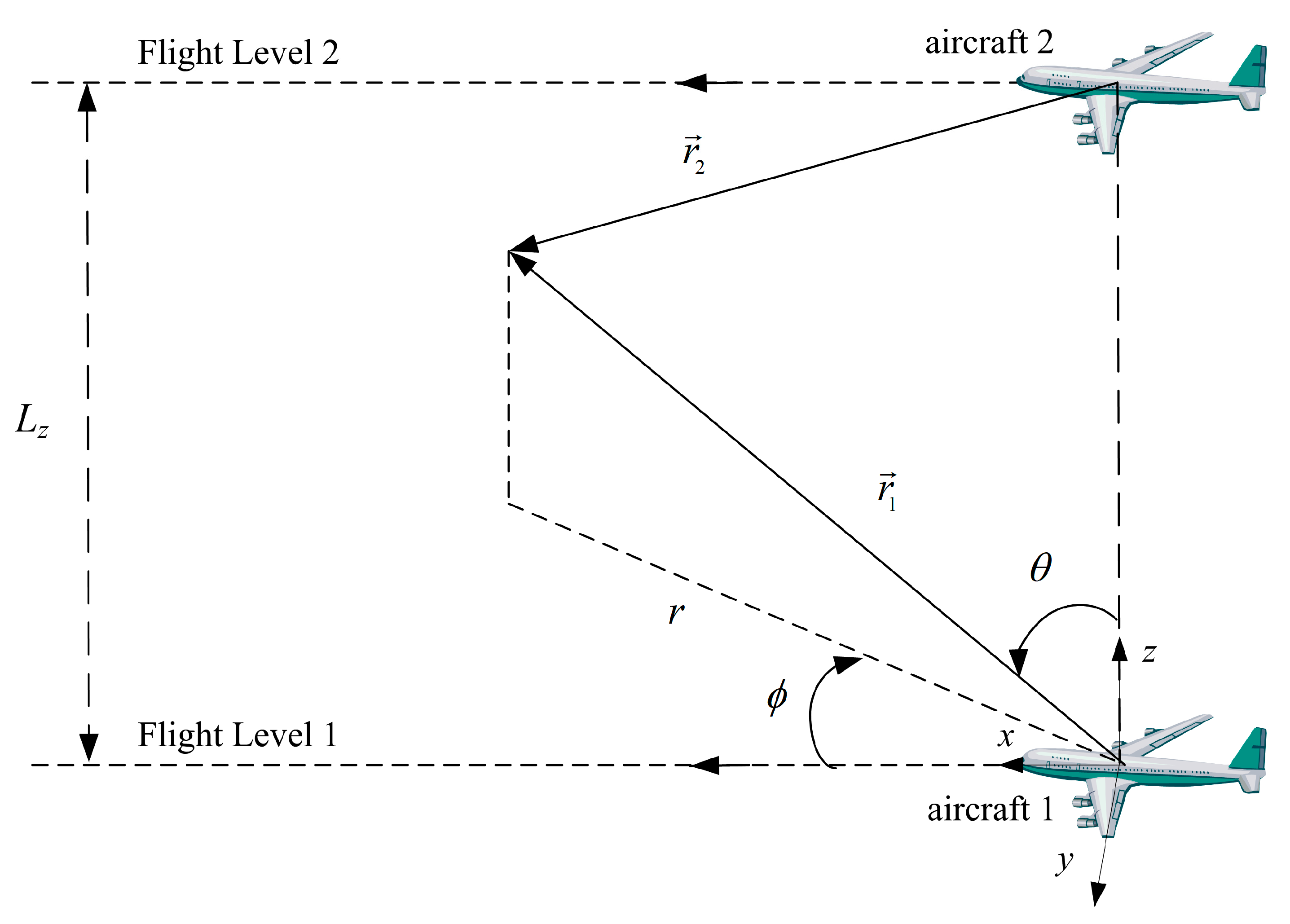
distance (1b) from aircraft “1”
r i position vector of the aircraft “i” respectively, (1b) and (2b) for i = 1, 2
r m distance of maximum probability of coincidence (7a; 8b)
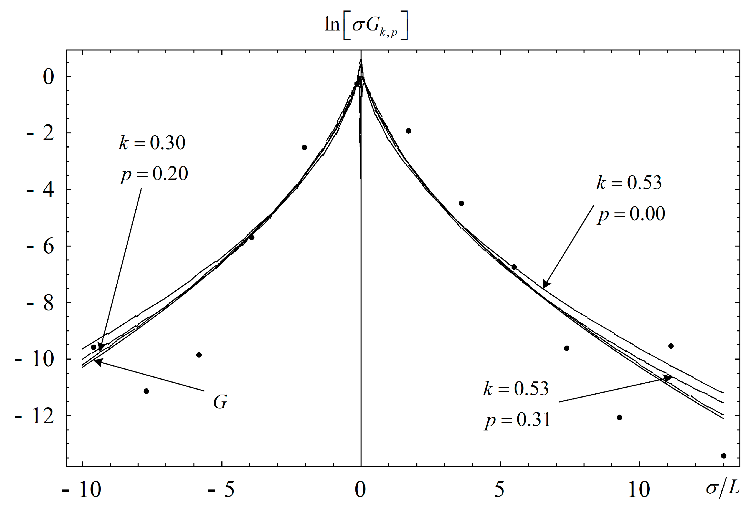
z m position (62a) of the minimum G m in (62b) of the function G in (60)
Aconstant factor (56a) in the generalized exponential probability distribution (54)
Ccorrection factor (65) between the Gaussian k = 2.0 and generalized exponential probability distribution with k = 1/2
Ddistance flown (47)
Fgeneralized exponential probability distribution (54) with weight k = 1/2 in (57)
Gratio (60) of generalized exponential probability distribution (57) with weight k = 1/2 to the Gaussian distribution (59) with weight k = 2.0
G m minimum (62b) of the function G in (60)
I 0 azimuthal integral (15) appearing in the three-dimensional cumulative probability of coincidence (13,14)
I ± radial integrals (18a) appearing in the evaluation of the three-dimensional cumulative probability of coincidence (13, 17)
L separation distance between aircraft (2b), e.g., standard (40a) or reduced (40b) vertical separation
P generalized exponential distribution (54; 56a,b) with (57) weight k = 1/2
P ¯ two-dimensional marginal probability of coincidence across the fight path (25b)
P = three-dimensional cumulative probability of coincidence over all space (13)
P i one-dimensional Gaussian probability distribution (1) of aircraft “i” as a function of position, respectively in (1a) and (2b) for i = 1, 2
P m maximum of the joint density of coincidence (11)
P 0 Laplace probability distribution (53)
P 12 joint probability density of coincidence (3)
Q k alternative ICAO target levels of safety for k = 1, 2, 3 using different units in, respectively, (45), (46) and (47)
R ¯ two-dimensional probability of coincidence for a great circle tour of the earth (49b)
S ICAO Target Level of Safety (43)
S = modified ICAO TLS (52b) based on the three-dimensional probability of coincidence over all space (13)
S m modified ICAO TLS (50a) based on maximum probability of coincidence (11)
T flight duration in hours (46)
V airspeed (45)
X m maxima probability of coincidence for a great circle tour of the earth (51)
ϕ polar angle (1b) in Figure 1
λ ratio r.m.s. position errors (33c)
σ i r.m.s. position error of the aircraft “i” appearing respectively in (1a) and (2a) for i = 1, 2
σ ¯ arithmetic mean of variances (30a) or squares of the r.m.s. position errors
θ azimuthal angle (1b) in Figure 1 and Figure 2.
θ m azimuthal angle of maximum probability of coincidence (7a)
ξ constant (21b) appearing in the evaluation of the integrals (18a)
ζ change of variable (21a) used to evaluate the integrals (18a)
Subscripts
1first aircraft
2second aircraft
astandard vertical separation of 2000 ft
breduced vertical separation of 1000 ft
Abbreviations
r.m.s.root mean square
ATMAir Traffic Management
ICAOInternational Civil Aviation Organization
TLSTarget Level of Safety
RVSMReduced Separation Vertical Minima
T-CASTraffic Collision Avoidance System

References

  1. Eurocontrol. EUROCONTROL Seven-Year Forecast February 2018. Available online: https://www.eurocontrol.int/sites/default/files/content/documents/official-documents/forecasts/seven-year-flights-service-units-forecast-2018-2024-Feb2018.pdf (accessed on 20 December 2020).
  2. Vismari, L.F.; Junior, J.B.C. A safety assessment methodology applied to CNS/ATM-based air traffic control system. Reliab. Eng. Syst. Saf. 2011, 7, 727–738. [Google Scholar] [CrossRef]
  3. Barnett, A. Free-Flight and en Route Air Safety a First-Order Analysis. Oper. Res. 2000, 48, 833–845. [Google Scholar] [CrossRef]
  4. Hinton, D.A.; Tatnall, C.R. A Candidate Wake Vortex Strength Definition for Application to the NASA Aircraft Vortex Spacing System (AVOSS); NASA: Hampton, VA, USA, 1997. [Google Scholar]
  5. Spalart, P.R. Airplane Trailing Vortices. Annu. Rev. Fluid Mech. 1998, 39, 107–138. [Google Scholar] [CrossRef]
  6. Rossow, V.J. Lift-generated vortex wakes of subsonic transport aircraft. Prog. Aerosp. Sci. 1999, 35, 507–660. [Google Scholar] [CrossRef]
  7. Campos, L.M.B.C.; Marques, J.M.G. On wake vortex response for all combinations of five classes of aircraft. Aeronaut. J. 2004, 108, 295–310. [Google Scholar] [CrossRef]
  8. Campos, L.M.B.C.; Marques, J.M.G. On the compensation and damping of roll induced by wake vortices. Aeronaut. J. 2014, 118, 1–23. [Google Scholar] [CrossRef]
  9. Campos, L.M.B.C.; Marques, J.M.G. On an analytical model of wake vortex separation of aircraft. Aeronaut. J. 2016, 120, 1534–1565. [Google Scholar] [CrossRef]
  10. ICAO. The Procedures for Air Navigation Services—Air Traffic Management (PANS-ATM), ICAO Doc 4444, 15th ed.; ICAO: Montreal, QC, Canada, 2009. [Google Scholar]
  11. Ballin, M.G.; Wing, D.J.; Hughes, M.F.; Conway, S.R. Airborne Separation Assurance and Air Traffic Management: Research and Concepts and Technology; AIAA: Reston, VA, USA, 1999. [Google Scholar]
  12. Anderson, E.W. Principles of Navigation; Hollis & Carter: London, UK, 1966. [Google Scholar]
  13. Leighton, S.J.; McGregor, A.E.; Lowe, D.; Wolfe, A.; Macaulay, A.A. GNSS Guidance for all Phases of Flight: Pratical Results. J. Navig. 2001, 54, 1–13. [Google Scholar] [CrossRef]
  14. Tomlin, C.; Pappas, J.; Sastry, S. Conflict Resolution in Air Traffic Management: A Study in Multi-agent Hybrid Systems. IEEE Trans. Autom. Control 1998, 43, 509–521. [Google Scholar] [CrossRef] [Green Version]
  15. Reich, P.G. Analysis of Long-range Air Traffic Systems: Separation Standards. J. Navig. 1966, 19, 88–98, 169–186, 331–347. [Google Scholar] [CrossRef]
  16. Eurocontrol. European Studies of Vertical Separation above FL290—Summary Report; Eurocontrol: Brussels, Belgium, 1988. [Google Scholar]
  17. Harisson, D.; Moek, G. European Studies to Investigate the Feasibility of using 1000 ft Vertical Separation Minima above FL 290: Part I: Overview of Organization, Techniques Employed and Conclusions. J. Navig. 1992, 44, 91–106. [Google Scholar] [CrossRef]
  18. Harisson, D.; Moek, G. European Studies to Investigate the feasibility of using 1000 ft Vertical Separation Minima above FL 290: Part II: Precision Data Analysis and Collision Risk Assessment. J. Navig. 1992, 45, 91–106. [Google Scholar] [CrossRef]
  19. Moek, G.; ten Have, J.M.; Harisson, D.; Cox, M.E. European Studies to Investigate the Feasibility of using 1000 ft Vertical Separation Minima above FL 290: Part III: Overview of Organization, Techniques Employed and Conclusions. J. Navig. 1992, 46, 245–261. [Google Scholar] [CrossRef]
  20. Campos, L.M.B.C. On the probability of collision between aircraft with dissimilar position errors. J. Aircr. 2001, 38, 593–599. [Google Scholar] [CrossRef]
  21. Campos, L.M.B.C.; Marques, J.M.G. On Safety Metrics Related to Aircraft Separation. J. Navig. 2002, 55, 39–63. [Google Scholar] [CrossRef]
  22. Shortie, J.F.; Xie, Y.; Chen, C.H.; Dunohue, G.L. Simulating Collision Probabilities of Landing Airplanes at Non-Towered Airports. Simulation 2004, 80, 21–31. [Google Scholar] [CrossRef]
  23. Houck, S.; Powell, J.D. Assessment of Probability of Mid-Air Collision during an Ultra Closely Spaced Parallel Approach; AIAA: Reston, VA, USA, 2001. [Google Scholar]
  24. Vidal, R.J.; Curtis, J.T.; Hilton, J.H. The Influence of Two-Dimensional Stream Shear on Airfoil Maximum Lift; Cornell Aeronautical Research Laboratory: Buffalo, NY, USA, 1961. [Google Scholar]
  25. Clodman, J.; Muller, F.R.; Morrisey, E.G. Wind Regime in the Lowest One Hundred Meters as Related to Aircraft Take-Offs and Landings. In Proceedings of the World Health Organization Conference, London, UK; 1968; pp. 28–43. [Google Scholar]
  26. Glazunov, V.G.; Guerava, V.Z. A Model of Windshear in the Lower 50 Meter Section of the Glide Path, from Data of Low Inertia Measurements; NLL-M-23036; Mathematical London Library of Science and Technology: London, UK, 1973. [Google Scholar]
  27. Gerlach, O.H.; Van de Moesdisk, G.A.J.; Van der Vaart, J.C. Progress in Mathematical Modeling of Flight in Turbulence; AGARD: Neuilly sur Seine, France, 1973. [Google Scholar]
  28. Etkin, B. Turbulent Wind and its Effects on Flight. J. Aircr. 1981, 18, 327–345. [Google Scholar] [CrossRef]
  29. Schanzer, G. Dynamic Energy Transfer between Wind and Aircraft. In Proceedings of the 13th Congress of the International Council of the Aeronautical, Seattle, WA, USA, 22–27 August 1982. [Google Scholar]
  30. Campos, L.M.B.C. On the Influence of Atmospheric Disturbances on Aircraft Aerodynamics. Aeronaut. J. 1984, 6, 257–264. [Google Scholar]
  31. Campos, L.M.B.C. On the Aircraft Flight Performance in a Perturbed Atmosphere. Aeronaut. J. 1986, 10, 301–312. [Google Scholar]
  32. Campos, L.M.B.C. On a Pitch Control Low for Constant Glide Slope through Windshears and Other Disturbances. Aeronaut. J. 1989, 9, 290–300. [Google Scholar]
  33. Etkin, B.; Etkin, D.A. Critical Aspect of Trajectory Prediction Flight in a Non-Uniform Wind; AGARD: Neuilly sur Seine, France, 1990. [Google Scholar]
  34. Pinsker, W.J.G. Critical Flight Conditions and Loads Resulting from Inertia Cross-Coupling and Aerodynamic Deficiencies; Aeronautical Research Council: London, UK, 1958. [Google Scholar]
  35. Hacker, T.; Oprisiv, C. A discussion of the roll coupling problem. Prog. Aerosp. Sci. 1974, 15, 30–60. [Google Scholar] [CrossRef]
  36. Schy, A.A.; Hannah, M.E. Prediction of jump phenomena in roll-coupling maneuvers of airplane. J. Aircr. 1975, 14, 100–115. [Google Scholar]
  37. Campos, L.M.B.C.; Aguiar, A.J.M.N. On the inverse phugoid problem as an instance of non-linear stability in pitch. Aeronaut. J. 1989, 10, 241–253. [Google Scholar]
  38. Campos, L.M.B.C.; Fonseca, A.A.; Azinheira, J.R.C. Some Elementary Aspects of Non-linear Airplane Speed Stability in Constrained Flight. Prog. Aerosp. Sci. 1995, 31, 137–169. [Google Scholar] [CrossRef]
  39. Etkin, B.; Reid, L.D. Dynamics of Flight: Stability and Control; Wiley: Hoboken, NJ, USA, 1996. [Google Scholar]
  40. Campos, L.M.B.C.; Azinheira, J.R.C. On the application of special functions to non-linear and unsteady stability. Integral Transform. Spec. Funct. 2003, 14, 149–180. [Google Scholar] [CrossRef]
  41. Campos, L.M.B.C. On the non-linear longitudinal stability of symmetrical aircraft. J. Aircr. 1997, 36, 360–369. [Google Scholar] [CrossRef]
  42. Mises, R.V. Theory of Probability and Statistics; Academic Press: Cambridge, MA, USA, 1960. [Google Scholar]
  43. Lindeberg, J.W. Ueber der Exponential Gezetzes in der Wahrlicheinkalkulus. Z. Math. 1922, 15, 211–225. [Google Scholar] [CrossRef] [Green Version]
  44. Reiss, R.D.; Thomas, M. Statistical Analysis of Extreme Values: With Applications to Insurance, Finance, Hydrology and Other Fields, 3rd ed.; Birkhäuser Verlag: Basel, Switzerland, 2007. [Google Scholar]
  45. Johnson, N.L.; Balakrishnan, N. Continuous Univariate Probability Distributions; Wiley: New York, NY, USA, 1995. [Google Scholar]
  46. Campos, L.M.B.C.; Marques, J.M.G. On the Combination of the Gamma and Generalized Error Distribution with Application to Aircraft Flight Path Deviation. Commun. Stat. Theory Methods 2004, 3, 2307–2332. [Google Scholar] [CrossRef]
  47. Braff, R.; Shively, C. A Method of Over Bounding Ground Based Augmentation System Heavy Tail Error Distributions. J. Navig. 2005, 58, 83–103. [Google Scholar] [CrossRef]
  48. Kozubowski, T.J.; Podgórsi, K. Asymmetric Laplace Laws and Modelling of Financial Data. Math. Comput. Model. 2001, 34, 1003–1021. [Google Scholar] [CrossRef]
  49. Jammalamadaka, S.R.; Kozubowski, T.J. New Families of Wrapped Distributions for Modelling Skew Circular Data. Commun. Stat. Theory Methods 2004, 33, 2059–2074. [Google Scholar] [CrossRef]
  50. Campos, L.M.B.C.; Marques, J.M.G. Collision Probabilities, Aircraft Separation and Airways Safety, Aeronautics and Astronautics; Mulder, M., Ed.; InTech: Rijeka, Croatia, 2011; pp. 571–588. [Google Scholar]
  51. Campos, L.M.B.C. Generalized Calculus with Applications to Matter and Forces; CRC Press: Boca Raton, FL, USA, 2014. [Google Scholar]
  52. Abramowitz, M.; Stegun, I. Tables of Mathematical Functions; Dover: Mineola, NY, USA, 1965. [Google Scholar]
  53. Campos, L.M.B.C.; Marques, J.M.G. On the Probability of Collision Between Climbing and Descending Aircraft. J. Aircr. 2007, 44, 550–557. [Google Scholar] [CrossRef]
  54. Campos, L.M.B.C.; Marques, J.M.G. On a dimensionless alternative to the ICAO Target Level of Safety. Proc. Inst. Mech. Eng. Part G J. Aerosp. Eng. 2016, 9, 1548–1557. [Google Scholar] [CrossRef]
  55. Pérez-Castán, J.A.; Rodríguez-Sanz, Á.; Pérez Sanz, L.; Arnaldo Valdés, R.M.; Gómez Comendador, V.F.; Greatti, C.; Serrano-Mira, L. Probabilistic Strategic Conflict-Management for 4D Trajectories in Free-Route Airspace. Entropy 2020, 22, 159. [Google Scholar] [CrossRef] [PubMed] [Green Version]
  56. Ribeiro, M.; Ellerbroek, J.; Hoekstra, J. Review of Conflict Resolution Methods for Manned and Unmanned Aviation. Aerospace 2020, 7, 79. [Google Scholar] [CrossRef]
  57. Pérez-Castán, J.A.; Comendador, F.G.; Rodríguez-Sanz, A.; Valdés, R.M.A.; Águeda, G.; Zambrano, S.; Torrecilla, J. Decision framework for the integration of RPAS in non-segregated airspace. Saf. Sci. 2020, 130, 104860. [Google Scholar] [CrossRef]
  58. Pérez-Castán, J.A.; Comendador, F.G.; Rodríguez-Sanz, Á.; Valdés, R.M.A.; Alonso-Alarcon, J.F. Safe RPAS integration in non-segregated airspace. Aircr. Eng. Aerosp. Technol. 2020, 6, 801–806. [Google Scholar] [CrossRef]
  59. Tabassum, A.; Sabatini, R.; Gardi, A. Probabilistic Safety Assessment for UAS Separation Assurance and Collision Avoidance Systems. Aerospace 2019, 6, 19. [Google Scholar] [CrossRef] [Green Version]
  60. Zhang, J.; Zou, X.; Wu, Q.; Xie, F.; Liu, W. Empirical study of airport geofencing for unmanned aircraft operation based on flight track distribution. Transp. Res. Part C Emerg. Technol. 2020, 121, 102881. [Google Scholar] [CrossRef]
  61. Costea, M.-L.; Nae, C.; Apostolescu, N.; Costache, F.; Andrei, I.-C.; Stroe, G.-L.; Semenescu, A. Automatic Aircraft Collisions Algorithm Development for Civil Aircraft. In Proceedings of the 2020 10th International Conference on Advanced Computer Information Technologies, Deggendorf, Germany, 16–18 September 2020; pp. 98–103. [Google Scholar]
  62. Hashemi, S.M.; Botez, R.M.; Grigorie, T.L. New Reliability Studies of Data-Driven Aircraft Trajectory Prediction. Aerospace 2020, 7, 145. [Google Scholar] [CrossRef]
  63. Metz, I.C.; Mühlhausen, T.; Ellerbroek, J.; Kügler, D.; Van Gasteren, H.; Kraemer, J.; Hoekstra, J.M. Simulation Model to Calculate Bird-Aircraft Collisions and Near Misses in the Airport Vicinity. Aerospace 2018, 5, 112. [Google Scholar] [CrossRef] [Green Version]
  64. Campos, L.M.B.C.; Marques, J.M.G. On the probability of collision for crossing aircraft. Aircr. Eng. Aerosp. Technol. 2011, 5, 306–314. [Google Scholar] [CrossRef]
Figure 1. Using spherical coordinates (r, θ, ϕ) with origin on aircraft one, and polar axis along the flight path, the probability of coincidence depends on (r, θ) but not on ϕ, because the configuration is axisymmetric around the flight path.
Aerospace 08 00031 g001
Figure 2. Two aircraft flying along parallel straight flight path with constant separation distance Lz, with the first having a position drift r 1 and the second having a position drift r 2 leading to a coincidence anywhere in three dimensions.
Aerospace 08 00031 g002
Figure 3. Measurement probability altitude deviations of aircraft (dots) showing improving fits for (1) the generalized error distribution with exponent k = 0.53 (dotted line); (2) the combined Gamma and generalized error distribution with exponent k = 0.53 for the exponential and exponent p = 0.31 for the power (dashed line); (3) item with k = 0.3 and p = 2.0 (solid line); and (4) a probability distribution G combining two of the preceding with suitable weight. The simplest case (1) is sufficient to model the tail of the probability distribution.
Aerospace 08 00031 g003
Table 1. Since the aircraft dissimilarity function (33b) is unchanged by interchanging the two aircraft, the three values in (33a) apply to six values of the dissimilarity parameter (33c).
λ σ 1 / σ 2 139
f ( λ ) 15/3 = 1.666741/9 = 4.5556
1 / λ σ 2 / σ 1 11/31/9
Table 2. Upper bound to probabilities of collision assuming Gaussian probability distribution with vertical separation L a = 2000 ft. Three values of the dissimilarity parameter in (40) are used in the maximum Pm and of the 3D cumulative P = probability of coincidence, which was calculated for a vertical separation L = 2000 ft, for several values of the r.m.s. position error σ ¯ , which is calculated from (30a) as the arithmetic mean of the variances of the position errors of the two aircraft. The latter alone specifies the 2D marginal probability of coincidence across the flight path P ¯ , which can be compared directly with the original ICAO TLS standard and is independent of the aircraft dissimilarity factor.
Arithmetic Mean of Variances
σ ¯ (ft)
Maximum of the Joint Probability Density of Coincidence
P m a (per Square NM)
1D Marginal Probability of Coincidence
P ¯ a (per NM)
3D Cumulative Probability of Coincidence
P = a (Times NM)
λ = 9 , 1 / 9 λ = 3 , 1 / 3 λ = 1 λ = 1 λ = 3 , 1 / 3 λ = 9 , 1 / 9
1000 3.94 × 10 1.44 × 10 8.64 2.52 2.14 × 10 1 7.73 × 10 2 1.03 × 10 2
500 7.84 2.87 1.72 2.51 × 10 1 5.34 × 10 3 1.92 × 10 3 2.57 × 10 4
400 1.29 4.73 × 10 1 2.84 × 10 1 3.31 × 10 2 4.51 × 10 4 1.62 × 10 4 2.17 × 10 5
300 1.78 × 10 2 6.50 × 10 3 3.90 × 10 3 3.41 × 10 4 2.62 × 10 6 9.42 × 10 7 1.26 × 10 7
200 3.72 × 10 8 1.36 × 10 8 8.16 × 10 9 4.76 × 10 10 1.62 × 10 12 5.83 × 10 13 7.81 × 10 14
180 1.30 × 10 10 4.77 × 10 11 2.86 × 10 11 1.50 × 10 12 4.14 × 10 15 1.49 × 10 15 2.00 × 10 16
160 4.54 × 10 14 1.66 × 10 14 9.96 × 10 15 4.65 × 10 16 1.01 × 10 18 3.65 × 10 19 4.88 × 10 20
140 3.80 × 10 19 1.39 × 10 19 8.34 × 10 20 3.40 × 10 21 5.68 × 10 14 2.04 × 10 24 2.74 × 10 25
120 5.15 × 10 27 1.88 × 10 27 1.13 × 10 27 3.96 × 10 29 4.85 × 10 32 1.75 × 10 32 2.34 × 10 33
100 3.98 × 10 40 1.46 × 10 40 8.74 × 10 41 2.55 × 10 42 2.17 × 10 45 7.81 × 10 46 1.05 × 10 46
Table 3. Upper bound to probabilities of collision assuming Gaussian probability distribution with vertical separation L b = 1000 ft. See Table 2 for a reduced vertical separation L b = 1000 ft.
Arithmetic Mean of Variances
σ ¯ (ft)
Maximum of the Joint Probability Density of Coincidence
P m b (per Square NM)
1D Marginal Probability of Coincidence
P ¯ b (per NM)
3D Cumulative Probability of Coincidence
P = b (Times NM)
λ = 9 , 1 / 9 λ = 3 , 1 / 3 λ = 1 λ = 1 λ = 3 , 1 / 3 λ = 9 , 1 / 9
500 1.56 × 10 2 5.76 × 10 3.46 × 10 5.04 1.07 × 10 1 3.86 × 10 2 5.17 × 10 3
300 7.40 × 10 2.71 × 10 1.62 × 10 1.42 1.09 × 10 2 3.92 × 10 3 5.24 × 10 4
200 5.17 1.89 1.13 6.62 × 10 2 2.25 × 10 4 8.11 × 10 5 1.09 × 10 5
150 7.11 × 10 2 2.60 × 10 2 1.56 × 10 2 6.83 × 10 4 1.31 × 10 6 4.71 × 10 7 6.30 × 10 8
100 1.49 × 10 7 5.44 × 10 8 3.26 × 10 8 9.52 × 10 10 8.10 × 10 13 2.92 × 10 13 3.90 × 10 14
90 5.21 × 10 10 1.91 × 10 10 1.14 × 10 10 3.00 × 10 12 2.07 × 10 15 7.46 × 10 16 9.98 × 10 17
80 1.81 × 10 13 6.64 × 10 14 3.98 × 10 14 9.30 × 10 16 5.06 × 10 19 1.82 × 10 19 2.44 × 10 20
70 1.52 × 10 18 5.56 × 10 19 3.33 × 10 19 6.81 × 10 21 2.84 × 10 24 1.02 × 10 24 1.37 × 10 25
60 2.06 × 10 26 7.54 × 10 27 4.52 × 10 27 7.92 × 10 29 2.42 × 10 32 8.73 × 10 33 1.17 × 10 33
50 1.59 × 10 39 5.83 × 10 40 3.50 × 10 40 3.72 × 10 44 1.08 × 10 45 3.91 × 10 46 5.23 × 10 47
Table 4. Comparison of the International Civil Aviation Organization (ICAO) Target Level of Safety (TLS) applied to: (top) the one-dimensional marginal probability of coincidence along the flight path (25b); (middle) the maximum of the joint probability of coincidence (11); (bottom) the three-dimensional cumulative probability of coincidence over all space (13). In each case is considered; (left) the standard vertical separation L a = 2000 ft; (right) the reduced vertical separation L b = 1000 ft. For each of the six combinations of identical aircraft is indicated: (i) the assumed r.m.s. altitude position error; (ii) the corresponding probability of coincidence; (iii) the maximum speed that meets the ICAO TLS in the original or modified form; (iv) the probability of coincidence for a great circle tour of the earth.
QuantityUnitStandardReduced
Vertical separationft L a = 2000 L b = 1000
r.m.s. altitude errorft σ ¯ a = 180 σ ¯ b = 90
One-dimensional marginal probability of coincidence with λ = 1 (NM)−1 P ¯ a = 1.50 × 10 12 P ¯ b = 3.00 × 10 12
Maximum velocity to meet the ICAO TLSkt V a S P ¯ a = 3.33 × 10 3 V b S P ¯ b = 1.67 × 10 3
Probability of coincidence in a great circle tour of the earth- R ¯ a P ¯ a D 3.24 × 10 8 R ¯ b P ¯ b D 6.48 × 10 8
r.m.s. altitude errorft σ ¯ m a = 160 σ ¯ m b = 80
Probability density ofcoincidence with λ = 3 or λ = 1 / 3 (NM)−2 P m a = 1.66 × 10 14 P m b = 6.40 × 10 14
Maximum velocity to meet the ICAO TLS (50a)- V m a S m P m a = 5.48 × 10 2 V m b S m P m b = 2.79 × 10 2
Probability of coincidence in a great circle tour of the earth- X m a = P m a D 2 = 7.74 × 10 6 X m b = P m b D 2 = 2.99 × 10 5
r.m.s. altitude errorft σ = a = 400 σ = b = 200
Cumulative probability of coincidence with λ = 9 or λ = 1 / 9 NM P = a = 2.17 × 10 5 P = b = 1.09 × 10 5
Maximum velocity to meet the ICAO TLS (49b)- V = a P = a / S = = 4.34 × 10 3 V = b P = b / S = = 2.17 × 10 3
Table 5. Table 2 was calculated for a Gaussian probability distribution (59) and is recalculated for a generalized exponential probability distribution (57), using the correction factor (65).
Arithmetic Mean of Variances
σ ¯ (ft)
Correction Factor CMaximum of the Joint Probability
Density of Coincidence
C P m (per Square NM)
2D Marginal Probability of Coincidence
C P ¯ (per NM)
3D Cumulative Probability
of Coincidence
C P = (Times NM)
λ = 9 , 1 / 9 λ = 3 , 1 / 3 λ = 1 λ = 1 λ = 3 , 1 / 3 λ = 9 , 1 / 9
10001.71 × 10−16.732.461.484.31 × 10−13.66 × 10−21.32 × 10−21.76 × 10⁻³
5002.21 × 10−11.736.35 × 10−13.80 × 10−15.55 × 10−21.18 × 10−34.25 × 10−45.68 × 10⁻⁵
4006.95 × 10−18.97 × 10−13.29 × 10−11.97 × 10−12.30 × 10−23.14 × 10−41.13 × 10−41.51 × 10⁻⁵
3001.78 × 1013.17 × 10−11.16 × 10−16.94 × 10−26.06 × 10−34.66 × 10−51.68 × 10−52.24 × 10−6
2001.27 × 1064.71 × 10−21.72 × 10−21.03 × 10−26.02 × 10−42.05 × 10−67.38 × 10−79.89 × 10−8
1802.00 × 1082.60 × 10−29.55 × 10−35.72 × 10−33.00 × 10−48.29 × 10−72.98 × 10−74.00 × 10−8
1602.82 × 10111.28 × 10−24.69 × 10−32.81 × 10−31.31 × 10−42.85 × 10−71.03 × 10−71.38 × 10−8
1401.41 × 10165.34 × 10−31.95 × 10−31.17 × 10−34.78 × 10−57.98 × 10−82.87 × 10−83.85 × 10−9
1203.42 × 10231.76 × 10−36.42 × 10−43.86 × 10−41.35 × 10−51.66 × 10−85.98 × 10−98.00 × 10−9
1001.03 × 10364.09 × 10−41.50 × 10−48.98 × 10−52.62 × 10−62.23 × 10−98.02 × 10−101.08 × 10⁻¹⁰
Table 6. As in Table 2 for a reduced vertical separation L = 1000 ft (as in Table 3) with correction factor of the generalized error probability distribution relative to the Gaussian (as in Table 5).
Arithmetic Mean of Variances
σ ¯ (ft)
Correction
Factor C
Maximum of the Joint Probability
Density of Coincidence
C P m (per Square NM)
2D Marginal Probability of Coincidence
C P ¯ (per NM)
3D Cumulative Probability
of Coincidence
C P = (Times NM)
λ = 9 , 1 / 9 λ = 3 , 1 / 3 λ = 1 λ = 1 λ = 3 , 1 / 3 λ = 9 , 1 / 9
5001.71 × 10−12.70 × 109.845.918.61 × 10−11.83 × 10−26.60 × 10−38.84 × 10⁻⁴
3001.47 × 10−11.09 × 103.992.392.09 × 10−11.61 × 10−35.77 × 10−47.72 × 10⁻⁵
2006.95 × 10−13.591.317.86 × 10−14.60 × 10−21.56 × 10−45.64 × 10−57.58 × 10−6
1501.78 × 101.264.62 × 10−12.77 × 10−11.21 × 10−22.33 × 10−58.38 × 10−61.12 × 10⁻⁶
1001.27 × 1061.89 × 10−16.89 × 10−24.13 × 10−21.20 × 10−31.03 × 10−63.70 × 10−74.94 × 10−8
902.00 × 1081.04 × 10−13.82 × 10−22.28 × 10−26.00 × 10−44.14 × 10−71.49 × 10−72.00 × 10−8
802.82 × 10115.11 × 10−21.8 × 10−21.12 × 10−22.63 × 10−41.43 × 10−75.14 × 10−86.89 × 10−9
701.41 × 10162.14 × 10−27.82 × 10−34.68 × 10−39.57 × 10−53.99 × 10−81.43 × 10−81.93 × 10−9
603.42 × 10237.04 × 10−32.58 × 10−31.55 × 10−32.71 × 10−58.27 × 10−92.98 × 10−94.00 × 10−10
501.03 × 10361.63 × 10−35.89 × 10−43.60 × 10−43.82 × 10−61.11 × 10−94.02 × 10−105.37 × 10⁻¹¹
Publisher’s Note: MDPI stays neutral with regard to jurisdictional claims in published maps and institutional affiliations.

