Multi-Fidelity Optimization of a Composite Airliner Wing Subject to Structural and Aeroelastic Constraints

Abstract

Efficient optimization is a prerequisite to realize the full potential of an aeronautical structure. The success of an optimization framework is predominately influenced by the ability to capture all relevant physics. Furthermore, high computational efficiency allows a greater number of runs during the design optimization process to support decision-making. The efficiency can be improved by the selection of highly optimized algorithms and by reducing the dimensionality of the optimization problem by formulating it using a finite number of significant parameters. A plethora of variable-fidelity tools, dictated by each design stage, are commonly used, ranging from costly high-fidelity to low-cost, low-fidelity methods. Unfortunately, despite rapid solution times, an optimization framework utilizing low-fidelity tools does not necessarily capture the physical problem accurately. At the same time, high-fidelity solution methods incur a very high computational cost. Aiming to bridge the gap and combine the best of both worlds, a multi-fidelity optimization framework was constructed in this research paper. In our approach, the low-fidelity modules and especially the equivalent-plate methodology structural representation, capable of drastically reducing the associated computational time, form the backbone of the optimization framework and a MIDACO optimizer is tasked with providing an initial optimized design. The higher fidelity modules are then employed to explore possible further gains in performance. The developed framework was applied to a benchmark airliner wing. As demonstrated, reasonable mass reduction was obtained for a current state of the art configuration.

1. Introduction

Ever since the early years of aviation, the design, analysis, and optimization of aircraft structures has been receiving ever-increasing attention from the scientific community and has, therefore, been subjected to extensive research studies. As a result, a wide variety of multi-fidelity computational tools, with application to a plethora of analysis disciplines, has emerged. During an aircraft design process, consisting mainly of the conceptual, preliminary and detailed design stages [1], the various computational tools are designated to a corresponding design stage mainly based on the computational time, the modeling complexity and the ability to capture the physical phenomena present. Early on, low-fidelity models, associated with fast turnaround times, yet incapable of modeling higher order phenomena, are employed, along with empirical knowledge, to steer the design towards optimality. As the design knowledge on the current candidate configuration matures, higher fidelity tools are employed, aiming to replicate the relevant phenomena with greater accuracy, albeit at an elevated and often prohibitive computational cost. Throughout the stages, all relevant tools are coupled with optimization algorithms in order to gain further knowledge regarding the design space, as well as to obtain the corresponding optimized solution.

A key enabler to the mass reduction trend of aeronautical structures is the rise of composite materials in the aeronautics field. Lighter yet stiffer configurations have emerged with improved static and dynamic aeroelastic response through tailoring of their properties [2]. One of the main challenges, nevertheless, remains the optimization of such structures, since the introduction of composite materials induces further computational and algorithmic complexity. On one hand, ply angles and thicknesses can be expressed as design variables, resulting into a more complex and irregular design space, but with facilitated algorithmic applicability. On the other hand, the use of lamination parameters for optimization purposes has been extensively studied over the past few years. Miki and Sugiyama [3] was among the first to generate optimum designs of laminated composite plates for required in-plane and maximum bending stiffness, buckling strength and natural frequency utilizing lamination parameters. Fukunaga et al. [4] explored the effect of bend-twist coupling on the fundamental frequency of symmetric laminated plates, indicating that this type of coupling reduces the fundamental frequencies. The optimal laminate configuration that maximizes the fundamental frequencies was also obtained. In his work, Liu et al. [5] maximized the buckling load of composite materials panels using flexural parameters and compared its results with a stacking sequence optimization design generated via a genetic algorithm, indicating a close correlation between the two methods. In later works, efforts were directed towards closure of the up-to-then incomplete feasible design space of the lamination parameters [6], and the aeroelastic tailoring of regular and variable stiffness composite materials wings [7,8], as well as the stiffness optimization subject to aeroelastic constraints [9]. Macquart et al. [10], as well as Bordogna et al. [11], extended the capabilities of the state-of-the art lamination parameters optimization algorithms, introducing blending constraints in order to guarantee a certain degree of ply continuity inside a variable stiffness composite wing.

It becomes evident that various disciplines must be involved in the design optimization process of a modern airliner composite wing, the main contributors being the structural and aerodynamic analysis, since they significantly influence the performance and safety of wing structures. Additional disciplines may be included on a case by case basis. Regarding the structural representation, Finite Element Analysis (FEA) models are commonly used at the preliminary and detailed design stages, with reduced order, equivalent beam or plate models aiming to provide greater insight into the candidate configurations, as well as reduce the design space at an early stage of the design process. The equivalent plate methodology (EPM), often preferred due to its inherent facilitated coupling capabilities with concurrent aerodynamic and optimization codes, initially developed by Giles in a series of research papers [12,13,14], was proven to be a robust and accurate enough numerical tool for the structural analysis of aircraft wings, as the comparison with a 3D FEA wing model showed. Later on, Livne et al. [15] included the EPM in a multidisciplinary structural, aerodynamics and control analysis and optimization framework of a composite aircraft wing, and went on to also include transverse shear effects in the EPM formulation [16]. The large deformation non-linear static and dynamic behavior of wings via the EPM formulation was also studied by Livne and Navarro [17], with good correlation up to relatively large levels of loading being obtained. In their work, Kapania and Liu [18] introduced Legendre polynomials in the EPM in order to avoid the numerical ill-conditioning problem often accompanied by the usage of simple polynomials as trial functions. The accuracy and efficiency of the method was demonstrated via a series of static, as well as free, vibration loading scenarios. Through a series of works, Krishnamurthy and Eldred [19], Krishnamurthy and Tsai [20], Krishnamurthy [21] developed an optimization framework for obtaining an equivalent plate by minimizing an error function accounting for the displacements and frequencies between the two numerical models under consideration. The methodology was initially tested in plates with and without discrete damage and was later used to evaluate the static and dynamic structural response of a baseline aircraft wing. In each case, an optimum thickness and concentrated mass distribution for the equivalent plate model was obtained. A scaling down methodology was also developed and put into test via a series of numerical tests. The developed methodology indicated that the static response of the wing structure was accurately predicted, with the equivalent plate model being capable of reproducing the first five frequencies of the wing structure within five percent. Over the last few years, Na and Shin [22], along with Henson and Wang [23], further enhanced the current EPM capabilities to account for control surfaces, as well as for tow steered composite wing skins, respectively.

On the other hand, implementation of dedicated computational analysis tools for the relevant disciplines into optimization frameworks is of paramount importance. Pioneering research was conducted by Triplett [24] and Love and Bohlman [25], where one of the earliest multidisciplinary design and optimization tool, aeroelastic Tailoring and Structural Optimization (TSO), was developed. The Rayleigh-Ritz EPM for the structural model, coupled with the Doublet Lattice Method were combined to optimize the thickness distribution and laminate orientations of a fighter wing subject to strength and flutter velocity constraints. Haftka [26] developed an automated procedure for the design and optimization of composite wings subject to strength and flutter constraints. A major conclusion drawn from this work was that the flutter speed may not be a continuous function of the structural stiffness; hence, in optimization under flutter constraint, the constraint should be formulated in terms of other, continuous parameters relative to the flutter phenomenon. Haftka [27] also coupled a lifting-line theory-based aerodynamics model with a wingbox FEA model to perform aeroelastic analysis and optimization of a wing under stress and drag constraints. Weight versus drag trade-off studies for aluminium and composite wings were conducted. It was found that the composite wings were associated with lower mass and drag but their increased flexibility resulted in a larger variation in drag in the Pareto front. One of the earliest aerostructural optimization analysis was performed by Grossman et al. [28], where, utilizing lifting-line aerodynamic models, along with beam equations for the structural representation, the optimum shape, and structural configuration of a sailplane wing was obtained. In a similar but more complex fashion, by means of numerical tools, Grossman et al. [29] optimized a transport aircraft wing, while in parallel developing methodologies for the calculation of the sensitivity derivatives, as well as a sequential approximate optimization module.

While optimization procedures using low-fidelity components for the representation of the structural and aerodynamic problem have to date offered major gains in the overall performance of wing structures, they have inherent limitations. The limitations result from the main assumptions of such methods; for aerodynamics, non-linearities are typically neglected and simplified wetted geometries are used. On the structural side, the assumption of linear behavior, together with simplified FEA models, sees widespread use in optimization. Increasing the fidelity of the aerodynamic and structural solvers can influence the optimization results [30] and represents a step beyond the current state-of-the-art [31,32]. For the coupled aeroelastic problem, linear approaches, both in terms of structure and aerodynamics represented in the frequency domain, are commonly used. Studying the dynamic aerostructural response with such formulations should be limited to linear or weakly non-linear cases due to the underlying assumptions. The dynamic response of wings that operate in the transonic region, as well as cases of boundary layer-shockwave interaction and flutter from flow separation (common in rotor blades), requires a high-fidelity representation of the aerodynamics to be accurately captured [33,34,35]. Even when the aeroelastic behavior is correctly captured, the increased detail in the unsteady aerodynamic loads can influence the optimum result. In Reference [36], different unsteady aerodynamic methods were used in a multi-fidelity aerostructural optimization of a helicopter rotor, leading to variation in the final optimum blade geometry. Even for the static aeroelastic case, differences due to varying fidelity of the aerodynamics solvers have indeed been pinpointed [37]. Furthermore, the presence of structural non-linearities can additionally have a serious effect on the aeroelastic behavior of a wing structure [38]. Such non-linearities are expected to become more common in the future due to the tendency to move to ever more efficient wings of very high-aspect ratio combined with highly flexible composite materials.

It becomes evident that the obtained optimized solution corresponds to a specific level of fidelity. Depending on the case, the assumptions in modeling each discipline can be justified. However, they could also represent an oversimplification of the actual physics of the problem and yield a sub-optimal design. The optimized solution can be in doubt due to the level of fidelity with which the various disciplines are approximated regardless of how tight the optimization constraints are set and how rigorous the optimization algorithm becomes. Thus, the fidelity of each component of the optimization framework must be carefully evaluated by taking into account the outstanding properties of each problem or by confirming the validity of the solution using higher fidelity analysis.

In the following brief overview, the emphasis will be mainly upon the impact of increasing the fidelity of the aerodynamic formulation. This is a conscious choice because solution and modeling procedures for even detailed 3D Shell-3D Beam Finite Element representations of the structure have become quite efficient. However, some examples covering the impact of high-fidelity structural modeling are also mentioned below.

Gains from the inclusion of high-fidelity analysis component to the optimization of future unconventional aircraft wing concepts have been reported in literature. In References [39,40], high-fidelity Computational Fluid Dynamics (CFD) was used to provide realistic predictions of engine-pylon-strut interference and viscous drag that was fed to the optimization procedure. Significant reduction in structural mass for a strut braced wing based upon the Common Research Model (CRM) wing planform was obtained by Variyar et al. [41] by using a complete multi-fidelity optimization framework that encompassed both high-fidelity aerodynamics and structural dynamics. For a similar aircraft configuration, the accurate derivation of aerodynamic loads is stressed as a crucial parameter by Variyar et al. [41] and a multi-fidelity approach even in conceptual stage deemed advantageous. Qian and Alonso [42] have included a high-fidelity structural model in an aerostructural optimization procedure to discover gains in range and a reduction in structural mass. Smith et al. [43] mention that including high-fidelity CFD and non-linear structural effects in the aeroelastic modeling of high aspect ratio wings can lead to important differences compared to linear methods. In this particular case, linear methods were found to lead to an overly conservative result for tip displacement and aerodynamic loads.

Unsurprisingly, most recently published studies regarding high-fidelity optimization frameworks deal with innovative wing configurations that are prone to aeroelastic instabilities (high-aspect ratio wings, transonic aircraft) and may also contain structural non-linearities. Quantifying the impact of higher-fidelity optimization to current state-of-the-art wings has not been as prominent in the literature. Liem et al. [44] have shown that significant benefits from high-fidelity aerostructural optimization can also be realized for current state-of-the-art wings.

The decision on the required analysis capabilities that dictates the adequate level of fidelity has important ramifications from a computational-cost perspective. Further numerical analysis with high-fidelity tools is typically performed to assess the validity of the low-fidelity results and support the decision on the adequate level of fidelity. This approach has been used in industry and research centers [45,46,47]. Multiple strategies to bridge the gap in computational cost and capabilities between high and low-fidelity potential flow solutions represented by the 3D Euler Equations and simple Vortex Lattice and Doublet Lattice Method (VLM and DLM) formulations, respectively have been presented in the literature. A practical approach is to employ medium-fidelity aerodynamics. This level of fidelity is represented by advanced 3D Panel Methods. These can allow for a more detailed geometrical modeling of aeronautical structures, including non-planar aerodynamic shapes. Furthermore, by employing advanced wake modeling techniques, reasonable approximations for re-circulation effects and induced drag can be achieved at a lower cost than high-fidelity solutions. Kennedy and Martins [48] have employed a 3D Panel Method in a parallel aerostructural optimization framework and have additionally checked the validity of the obtained aerodynamic solutions against high-fidelity ones. Mieloszyk and Goetzendorf-Grabowski [49] have used a 3D Panel method in conjunction with corrections for viscous effects to evaluate the flight dynamics stability constraints in the multidisciplinary optimization of a joined wing box configuration. Recently, a finite element beam model was coupled to 3D Panel Aerodynamics and employed in aeroelastic optimization by Conlan-Smith and Schousboe Andreasen [50].

A natural path to reduce the computational cost associated with increased fidelity is to search for an optimized solution in smaller regions of the parameter space (thus requiring a smaller number of optimization iterations). This approach requires a priori some knowledge of the region in parameter space where the optimum is likely to be detected. In our multi-fidelity optimization framework, the low-fidelity part is entrusted with obtaining an initial optimized design with a high numerical certainty. Then, the high-fidelity modules explore further gains in performance by modeling the physics that the low-fidelity modules cannot. Overall, only a fraction of the iterations using high-fidelity are performed (in the range of 5–10%). Such an approach prevents a drastic increase in computational cost. The procedure of gradually moving to increasing level of fidelity but with a smaller number of solutions is typical of a multi-fidelity optimization framework [51,52].

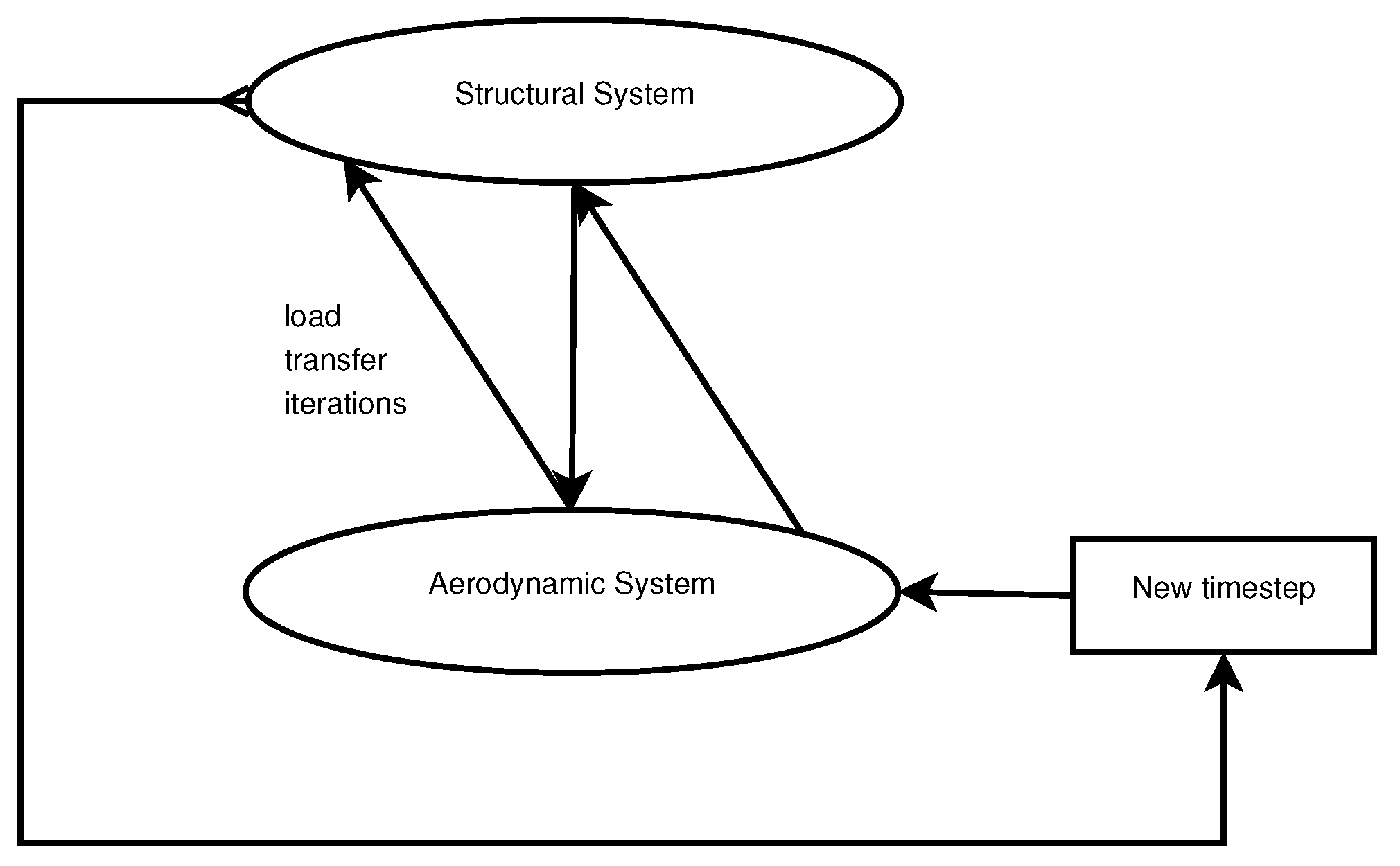
Still, a very high computational cost due to each high- fidelity solution is incurred, particularly so if a higher number of runs is needed. This cost is further exacerbated in the aeroelastic solutions. The cost of solving the unsteady aerodynamics with a high-fidelity method (typically a form of the Navier–Stokes equations with spatial approximation provided by the finite volume or element methods) tends to be higher than the structural solution. A combined computational cost of solving the structure and unsteady aerodynamics plus the interpolation of data between the two systems is then incurred. To mitigate this cost significantly, particularly for multiple runs around the same reference flow conditions, Order Reduction techniques can be used. Such techniques strive to approximate the physical behavior of the system on a greatly reduced (but physically meaningful) set of degrees of freedom. Most reduced order models are trained using samples from full solutions. The cost of obtaining those samples represents the main cost considering their use, since, afterward, they provide extremely rapid solution times. 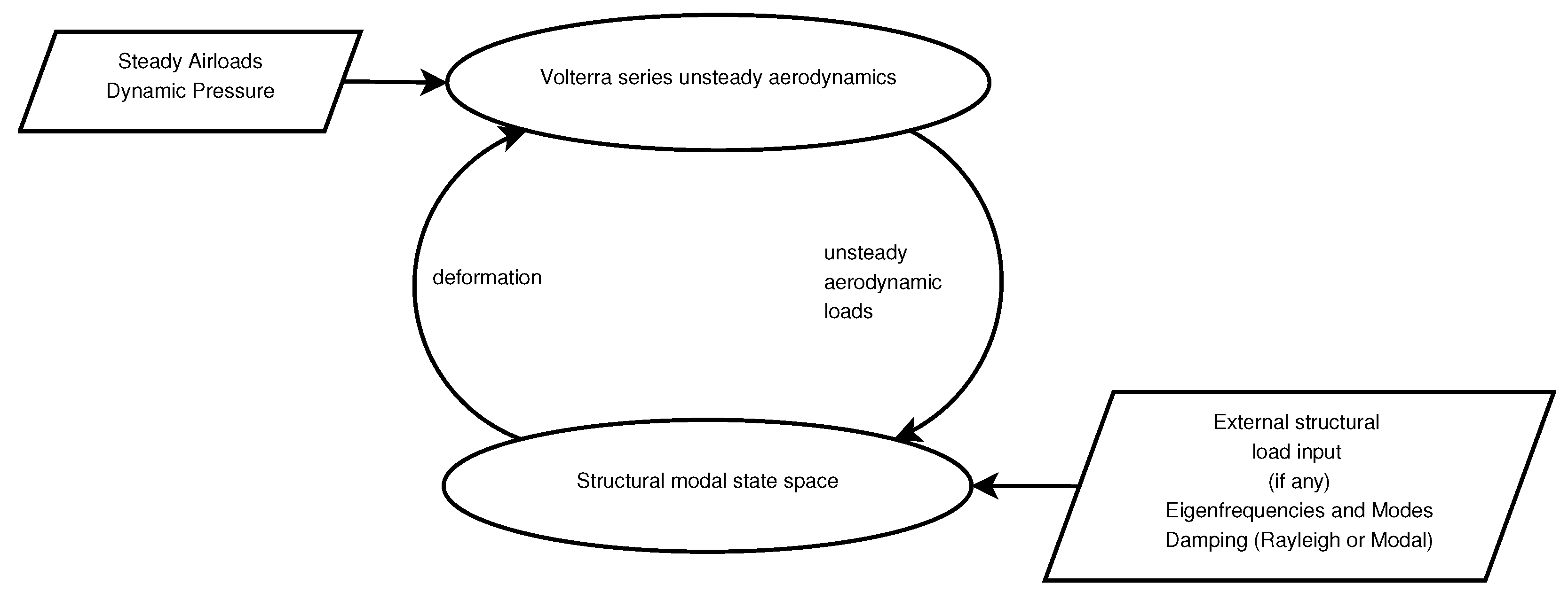Several types of reduced order models (ROMs) have been used to treat aeroelasticity, including those based on (a) Mathematical decompositions, such as proper orthogonal decomposition (POD) [53,54], (b) Series approximations (for example, Volterra or Wiener) [55], and (c) Machine Learning techniques [56]. In our work, we integrate a ROM to the optimization framework that uses a Volterra series approximation for the unsteady aerodynamics coupled with mode superposition on the structural side. It serves as an intermediate step between low-fidelity aeroelastic solutions and the full coupled high-fidelity final run.

Although multiple analysis techniques of varying fidelity have been successfully used in optimization, the different computational cost that they incur combined with their setup complexity leads to a different combination of methods being adopted in each design stage of an aircraft structure. Specifically in industry, the current state-of-the-art is to include higher fidelity modules as design maturity increases (preliminary and detailed design stages), while exploiting the low computational cost of low-fidelity methods in the conceptual stage [47,57]. In the conceptual stage, efficient low-fidelity methods (panel method aerodynamics and equivalent beam or plate structural models) are commonly preferred due to the requirement to evaluate the feasibility of a vast number of design configurations.

Advances in computational capabilities combined with robust and optimized high-fidelity analysis tools has resulted in a trend to incorporate such methods already from the preliminary stage. In order to bridge the gap between capabilities and computational cost between high and low-fidelity methods, two of the most attractive methodologies consist of employing correction factors to the lower-fidelity tools [37,58], as well as constructing surrogate models. Furthermore, the construction of multi-fidelity optimization frameworks represents a highly active research topic. Such frameworks strive to combine the advantages of both worlds while mitigating the associated computational cost [47].

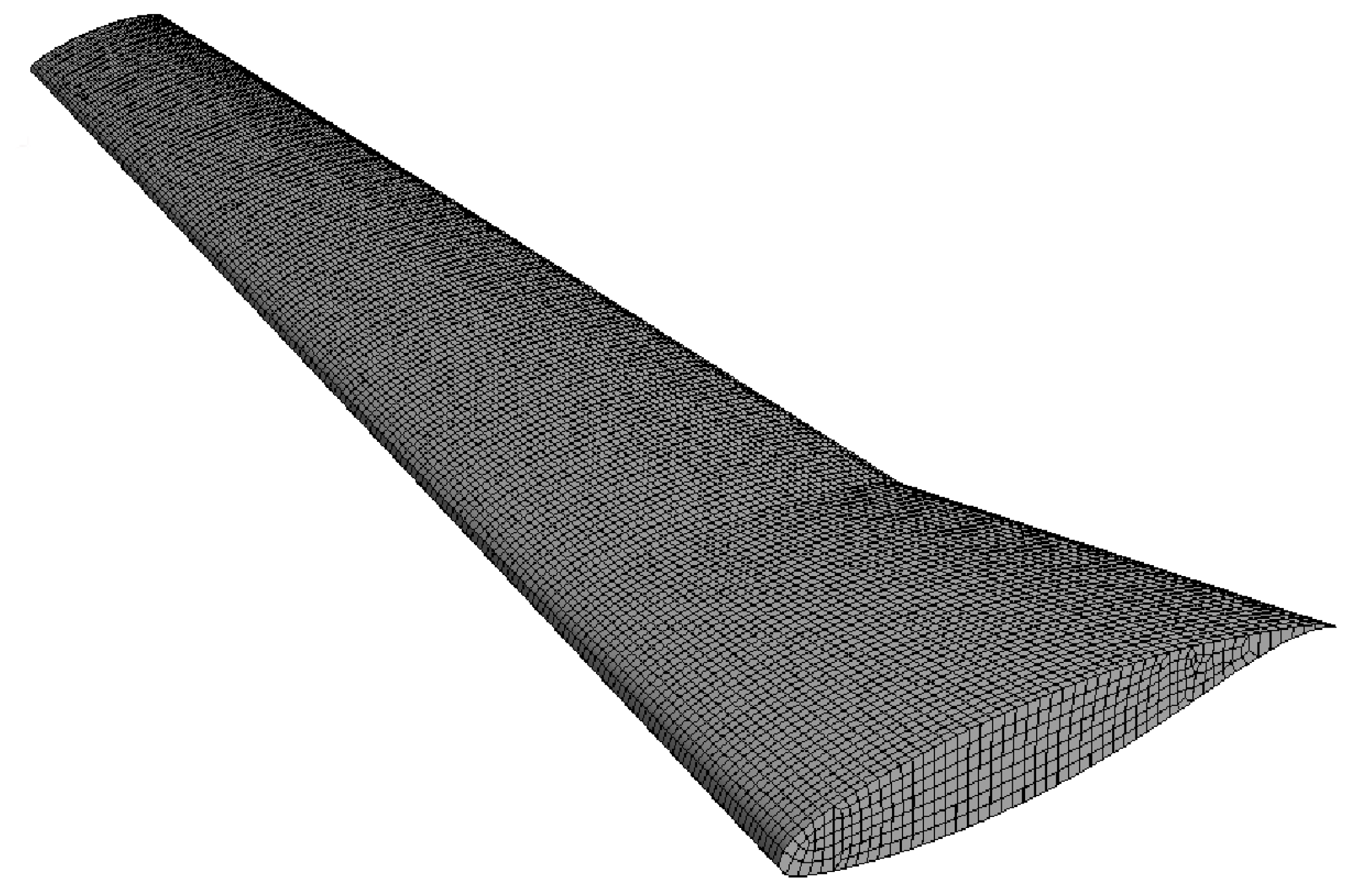
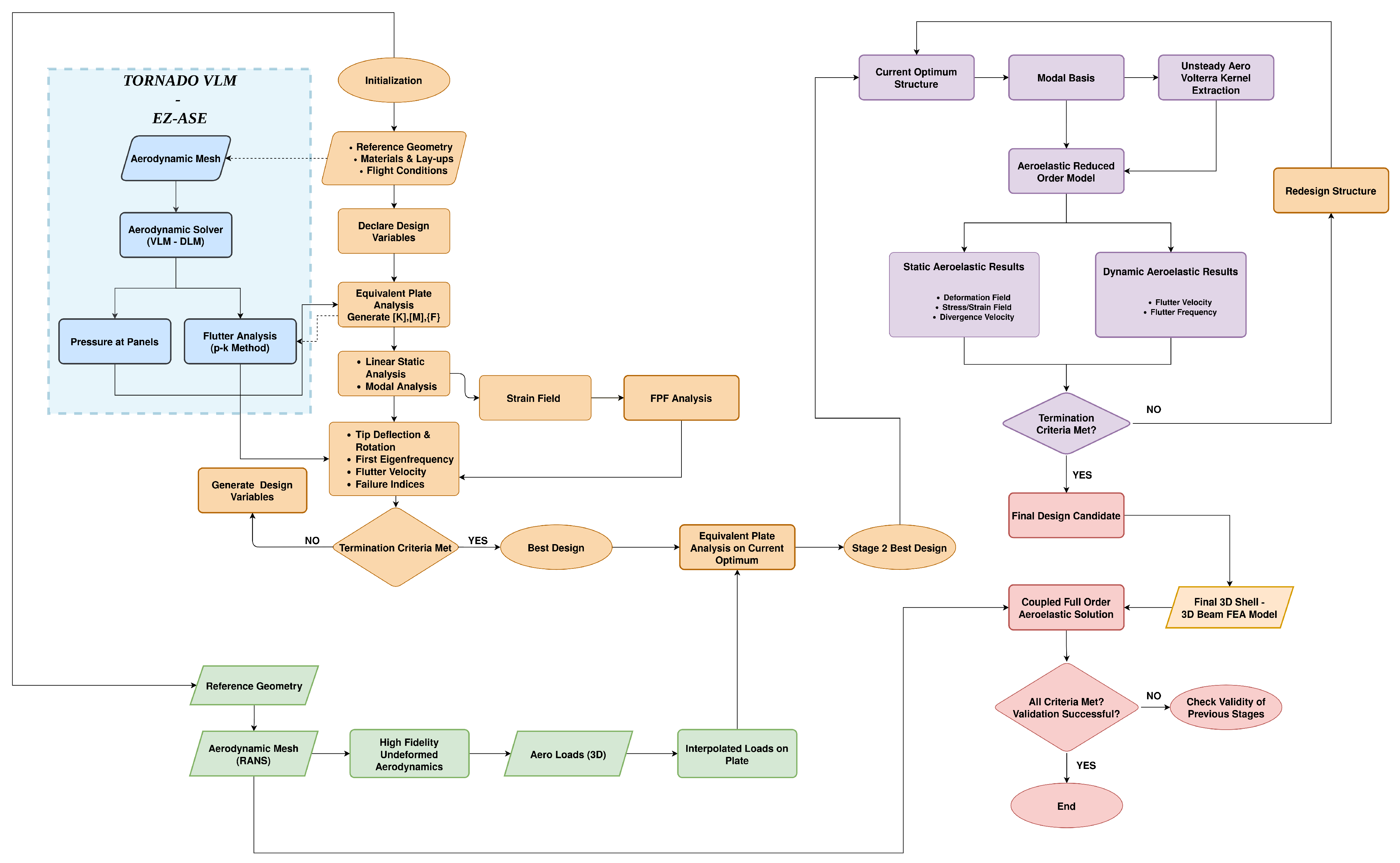
The primary research goal of the present study is to evaluate the gains in the structural optimization of a current state-of-the-art composite airliner wing by implementing a multi-fidelity optimization framework. Structural and aeroelastic constraints are used to formulate the optimization problem. The developed framework and the insight gained in the structural design and optimization of the composite wing model was used in the GRETEL project [59]. 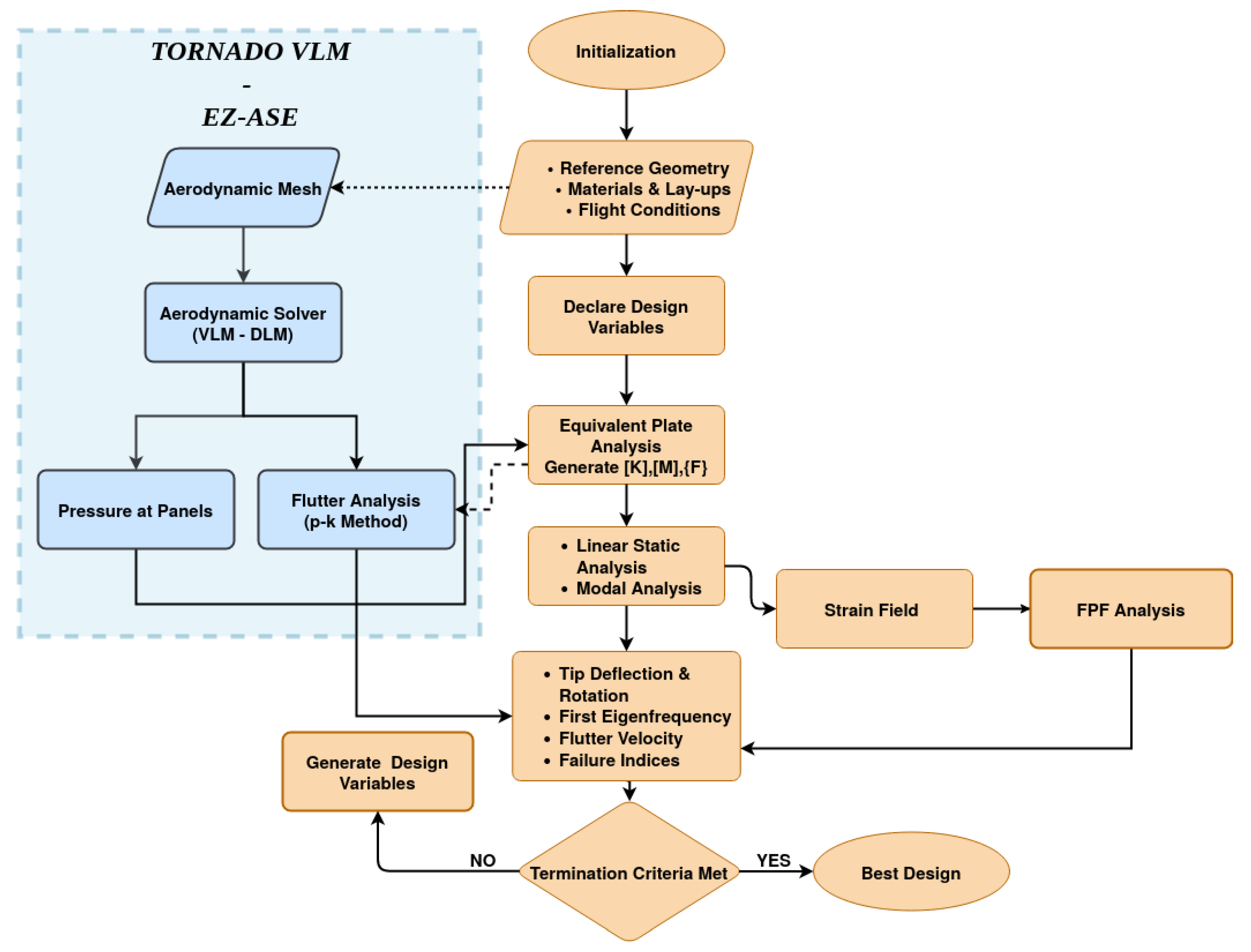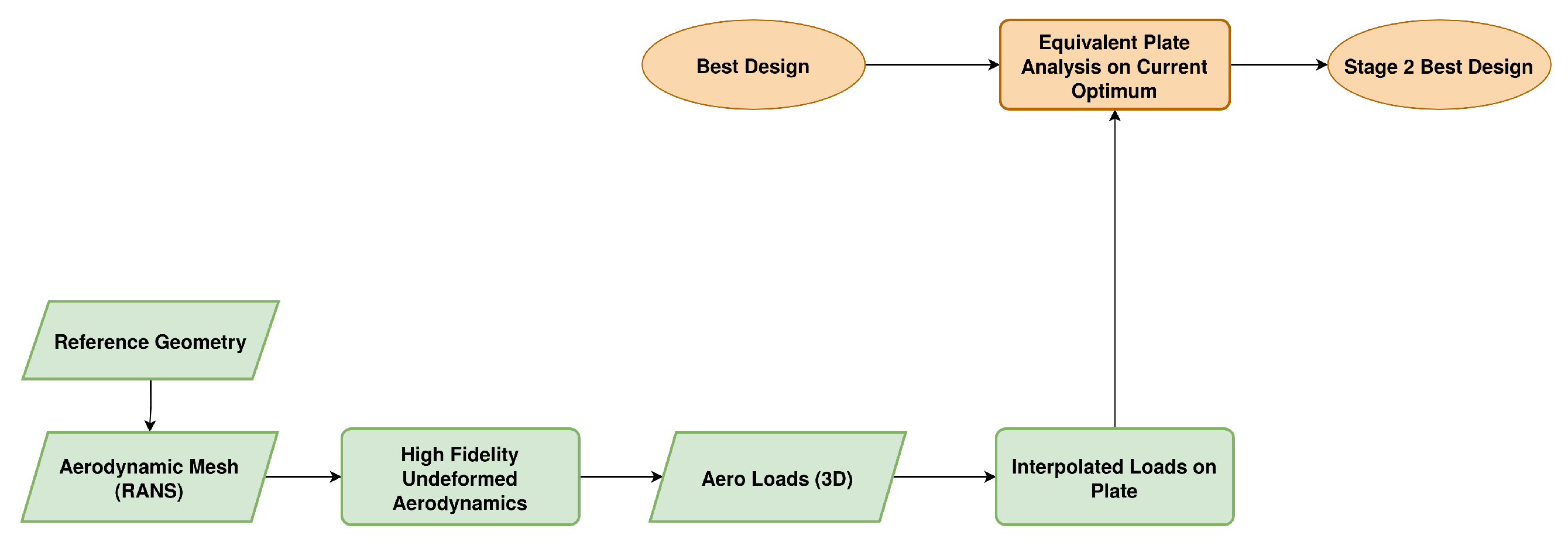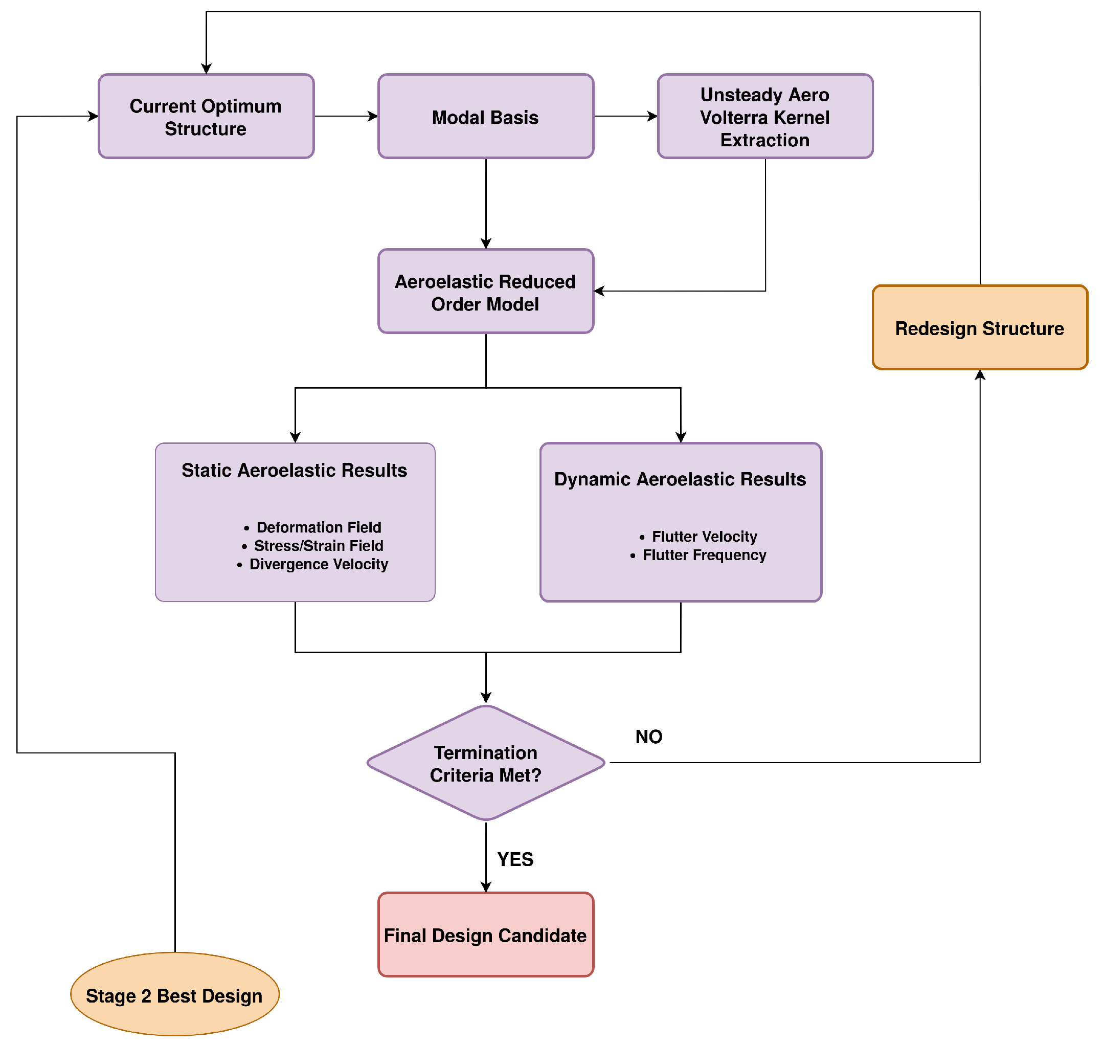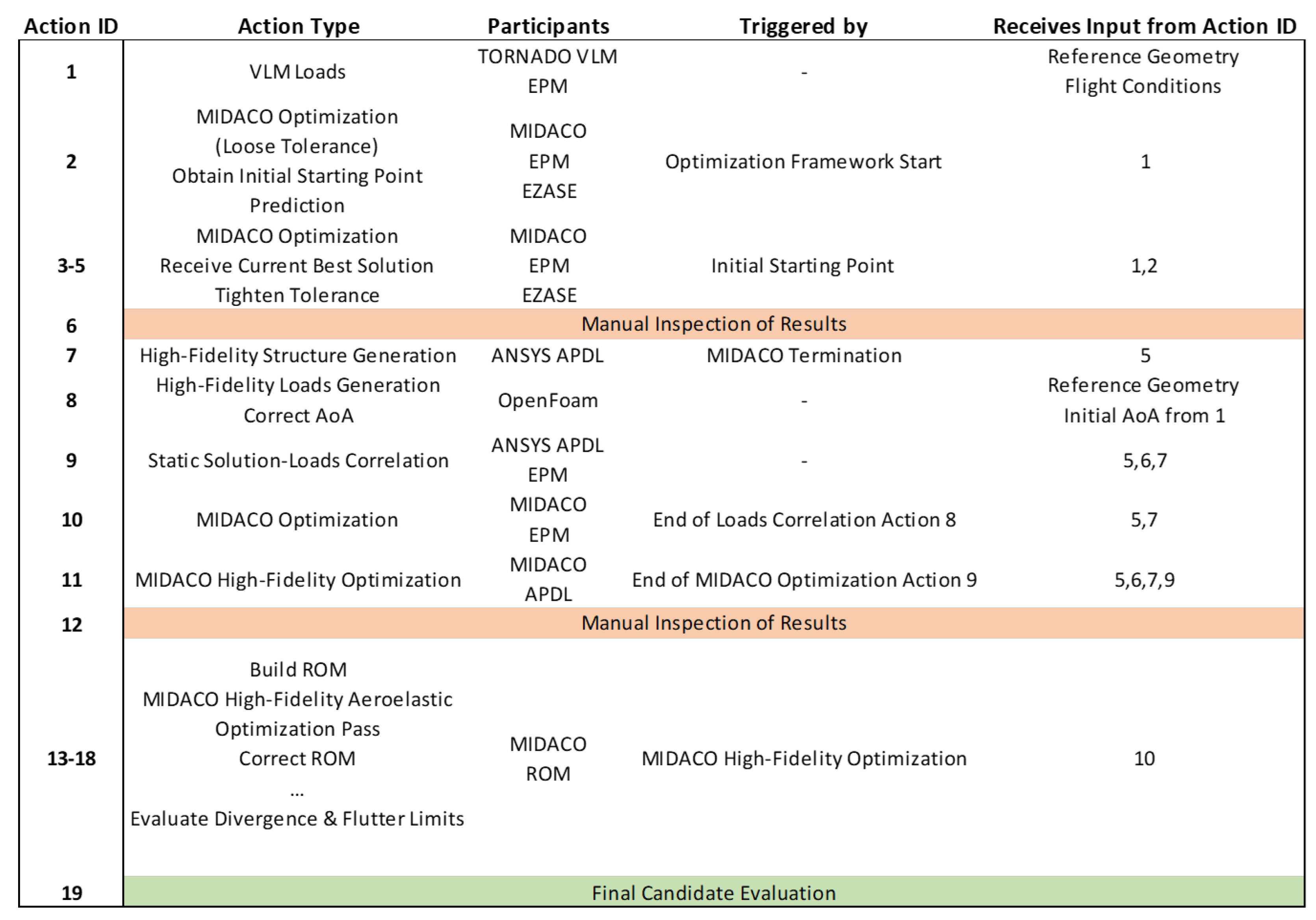As a case study, a modified, planar (untwisted) version of the Common Research Model (CRM) [60] wing has been treated. The optimization framework is based on the Equivalent Plate Model (EPM) and the Mixed Integer Ant Colony Optimization (MIDACO) algorithm. At the first stage, an optimized configuration for the wing under low-fidelity aerodynamic loading is obtained. Higher fidelity aerodynamic solutions are then generated, and possible changes in the optimized solution are explored. Finally, the static aeroelastic response of the wing under consideration is also investigated. An overview of the performed actions of the developed optimization framework for the current case study is presented in Appendix B, highlighting input-output relations.

Although multiple studies in the literature assess the gains of using multi-fidelity optimization frameworks for innovative wing configurations, the gains for the current-state-of-the-art wings are less prominently covered. The present study aims to contribute to closing this gap. We demonstrate that, through the use of this optimization tool, reasonable gains in structural mass of the test case wing were realized.

2. Materials and Methods

The developed multi-fidelity structural optimization framework is comprised of several distinct modules of varying fidelity and computational cost. The flowchart for the optimization framework is presented in Figure A4. These are combined in a manner that enables efficient turnaround times, as well as an optimized solution, with high levels of certainty accounting for the most relevant physics. In the next paragraphs, each of the consisting modules of the optimization framework will be mentioned, and their contribution, advantages, and disadvantages assessed. In addition, we will then present their combination in the developed optimization framework. The path from initial design to optimized solution referring to the potential changes at each separate stage will be described.

2.1. Low-Fidelity Modules

The present module, consisting mainly of low-fidelity computational tools and physics approximations, initializes the design process and, hence, is responsible for narrowing down the design space, while simultaneously steering the design towards optimum solutions, as well as accelerating the design procedure. The following sub-modules are included and described in detailed fashion:

• EPM Structural Model
• Low-Fidelity Aerodynamics
• Optimization Framework

2.1.1. EPM Structural Model

Starting from the cornerstone of this work, the EPM enables a great reduction in the dimensionality of the problem since under the assumption of a relatively small thickness-to-chord ratio one can assume that an aircraft wing pertains a plate-like behavior. The problem is then reduced from a 3D representation to a 2D equivalent plate with smeared properties, reducing the associated DOFs. Plate kinematics, and specifically the First Order Shear Deformation Theory (FSDT) [61], can be utilized to describe and calculate the stress and strain state of each wing component. In particular, the wing skins, spar, and rib webs are treated as laminated plates, while, on the other hand, and as per common practice, spar and rib caps are assumed to resist axial loads only and are, thus, considered as one-dimensional rods. To obtain the governing equation of the system the principle of minimum total potential energy is applied [18]. Under the FEA method, interpolation functions are used to describe the variation of the displacement field within an element, as well as to obtain the stiffness and mass matrices, $\left[\mathit{K}\right]$ and $\left[\mathit{M}\right]$, respectively. Another important assumption of the EPM is that the superposition principle holds; hence, the individual stiffness and mass matrices of each wing component can be summed in order to obtain the respective wing global matrices:

$$\begin{array}{cc}\hfill & {\left[\mathit{K}\right]}_{wing}={\left[\mathit{K}\right]}_{skin}+{\left[\mathit{K}\right]}_{spa{r}_{cap}^{web}}+{\left[\mathit{K}\right]}_{ri{b}_{cap}^{web}}\hfill \\ \hfill & {\left[\mathit{M}\right]}_{wing}={\left[\mathit{M}\right]}_{skin}+{\left[\mathit{M}\right]}_{spa{r}_{cap}^{web}}+{\left[\mathit{M}\right]}_{ri{b}_{cap}^{web}}\hfill \end{array}$$

(1)

Let F be a generic function that describes the stiffness and mass distribution along the three-dimensional space for each wing component. The contribution of each EPM element to the global matrices is derived via the following integrals. Gaussian numerical integration is employed for the solution of the integrals, along with a coordinate transformation between the physical coordinates $(x,y)$ and the generalized coordinates ($\xi$,$\eta$). The limits of integration in the through-the-thickness (z axis) coordinate correspond to the maximum extent of the local part of the actual wing structure.

$$\begin{array}{cc}\hfill & {\int \int \int }_{V}F(x,y,z)dV={\int }_{-1}^1{\int }_{-1}^1(\sum _{n=1}^{N_z}{\int }_{z_{in}}^{z_{jn}}F\left\{x\left(\xi ,\eta \right),y\left(\xi ,\eta \right),z\right\}\left|J\right|dz)d\xi d\eta ,\hfill \end{array}$$

(2)

where $N_z$ is the number of integration points in the z-direction, $z_{in}$ and $z_{jn}$ the integration limits of the n-th integration point, and $\left|J\right|$ the determinant of the Jacobian of the coordinate transformation. Each wing component pertains different geometric characteristics; hence, specific treatment is required for the integration procedure:

• Skins:

  $$\begin{array}{cc}\hfill & {\int \int \int }_{V}F\left(x,y,z\right)dV={\int }_{-1}^1{\int }_{-1}^1({\int }_{z_L-\frac{1}{2}{t}_L}^{z_L+\frac{1}{2}{t}_L}F·\left|J\right|dz+{\int }_{z_U-\frac{1}{2}{t}_U}^{z_U+\frac{1}{2}{t}_U}F·\left|J\right|dz)d\xi d\eta ,\hfill \end{array}$$

  (3)

  where $t_{L,U}=t_0\sqrt{1+{tan}^2{a}_{L,U}}$, the thickness of the upper and lower skins, respectively, and $a_{L,U}$ the local airfoil angle of the lower and upper skin, as illustrated in Figure 1a. For a laminated plate, the numerical integration in the z-direction is performed for each lamina individually, along with its corresponding constitutive matrix. The rest of the components contribute in an analogous manner, albeit the integration limits are modified according to their relevant geometric characteristics, as presented in Figure 1b.
• Spar Webs:

  $$\begin{array}{cc}\hfill & {\int \int \int }_{V}F\left(x,y,z\right)dV={\int }_{-1}^1{\int }_{{\xi }_s\left(n\right)-\frac{t_1}{c}}^{{\xi }_s\left(n\right)+\frac{t_1}{c}}{\int }_{z_L+\frac{1}{2}{t}_L+h_1}^{z_U-\frac{1}{2}{t}_U-h_1}F\left\{x\left(\xi ,\eta \right),y\left(\xi ,\eta \right),z\right\}\left|J\right|dzd\xi d\eta =\hfill \\ \hfill & {\int }_{-1}^1{\int }_{-1}^1\frac{t_1}{c}{\int }_{z_L+\frac{1}{2}{t}_L+h_1}^{z_U-\frac{1}{2}{t}_U-h_1}F\left\{x\left[\frac{t_1}{c}\xi +{\xi }_s\left(n\right),n\right],y\left[\frac{t_1}{c}\xi +{\xi }_s\left(n\right),n\right],z\right\}\left|J\right|dzd\xi d\eta \hfill \end{array}$$

  (4)
• Spar Caps:

  $$\begin{array}{cc}\hfill {\int \int \int }_{V}F\left(x,y,z\right)dV& ={\int }_{-1}^1{\int }_{{\xi }_s\left(n\right)-\frac{l_1}{c}}^{{\xi }_s\left(n\right)+\frac{l_1}{c}}({\int }_{z_L+\frac{1}{2}{t}_L}^{z_L+\frac{1}{2}{t}_L+h_1}F\left\{x\left(\xi ,\eta \right),y\left(\xi ,\eta \right),z\right\}\left|J\right|dz\hfill \\ \hfill & +{\int }_{z_U-\frac{1}{2}{t}_U-h_1}^{z_U-\frac{1}{2}{t}_U}F\left\{x\left(\xi ,\eta \right),y\left(\xi ,\eta \right),z\right\}\left|J\right|dz)d\xi d\eta =\hfill \\ \hfill & {\int }_{-1}^1{\int }_{-1}^1\frac{l_1}{c}({\int }_{z_L+\frac{1}{2}{t}_L}^{z_L+\frac{1}{2}{t}_L+h_1}F\left\{x\left[\frac{l_1}{c}\xi +{\xi }_s\left(n\right),n\right],y\left[\frac{l_1}{c}\xi +{\xi }_s\left(n\right),n\right],z\right\}\left|J\right|dz\hfill \\ \hfill & +{\int }_{z_U-\frac{1}{2}{t}_U-h_1}^{z_U-\frac{1}{2}{t}_U}F\left\{x\left[\frac{l_1}{c}\xi +{\xi }_s\left(n\right),n\right],y\left[\frac{l_1}{c}\xi +{\xi }_s\left(n\right),n\right],z\right\}\left|J\right|dz)d\xi d\eta \hfill \end{array}$$

  (5)
• Rib Webs:

  $$\begin{array}{cc}\hfill & {\int \int \int }_{V}F(x,y,z)dV={\int }_{-1}^1{\int }_{{\eta }_r\left(\xi \right)-\frac{t_2}{s}}^{{\eta }_r\left(\xi \right)+\frac{t_2}{s}}{\int }_{z_L+\frac{1}{2}{t}_L+h_2}^{z_U-\frac{1}{2}{t}_U-h_2}F\left\{x\left(\xi ,\eta \right),y\left(\xi ,\eta \right),z\right\}\left|J\right|dzd\xi d\eta =\hfill \\ \hfill & {\int }_{-1}^1{\int }_{-1}^1\frac{t_2}{s}{\int }_{z_L+\frac{1}{2}{t}_L+h_2}^{z_U-\frac{1}{2}{t}_U-h_2}F\left\{x\left[\xi ,\frac{t_2}{s}\eta +{\eta }_r\left(\xi \right)\right],y\left[\xi ,\frac{t_2}{s}\eta +n_r\left(\xi \right)\right],z\right\}\left|J\right|dzd\xi d\eta \hfill \end{array}$$

  (6)
• Rib Caps:

  $$\begin{array}{cc}\hfill {\int \int \int }_{V}F\left(x,y,z\right)dV& ={\int }_{-1}^1{\int }_{{\eta }_r\left(\xi \right)-\frac{l_2}{s}}^{{\eta }_r\left(\xi \right)+\frac{l_2}{s}}({\int }_{z_L+\frac{1}{2}{t}_L}^{z_L+\frac{1}{2}{t}_L+h_2}F\left\{x\left(\xi ,\eta \right),y\left(\xi ,\eta \right),z\right\}\left|J\right|dz\hfill \\ \hfill & +{\int }_{z_U-\frac{1}{2}{t}_U-h_2}^{z_U-\frac{1}{2}{t}_U}F\left\{x\left(\xi ,\eta \right),y\left(\xi ,\eta \right),z\right\}\left|J\right|dz)d\xi d\eta =\hfill \\ \hfill & {\int }_{-1}^1{\int }_{-1}^1\frac{l_2}{s}({\int }_{z_L+\frac{1}{2}{t}_L}^{z_L+\frac{1}{2}{t}_L+h_2}F\left\{x\left[\xi ,\frac{l_2}{s}\eta +{\eta }_r\left(\xi \right)\right],y\left[\xi ,\frac{l_2}{s}\eta +{\eta }_r\left(\xi \right)\right],z\right\}\left|J\right|dz\hfill \\ \hfill & +{\int }_{z_U-\frac{1}{2}{t}_U-h_2}^{z_U-\frac{1}{2}{t}_U}F\left\{x\left[\xi ,\frac{l_2}{s}\eta +{\eta }_r\left(\xi \right)\right],y\left[\xi ,\frac{l_2}{s}\eta +{\eta }_r\left(\xi \right)\right],z\right\}\left|J\right|dz)d\xi d\eta ,\hfill \end{array}$$

  (7)

where $h_1$,$h_2$ the thickness of a spar/rib cap, $l_1$,$l_2$ the width of a spar/rib cap, and $t_1$,$t_2$ the thickness of a spar/rib web, respectively.

2.1.2. Low-Fidelity Aerodynamics

One of the most attractive merits of the EPM is the facilitated coupling with contemporary aerodynamic panel methods, and specifically the Vortex Lattice Method (VLM) [62], since both methods are based on flat-plate representations of their respective discipline. The VLM, a well-established numerical method used in the early design stages of aircraft design, assumes an incompressible, inviscid and irrotational flow field, along with horseshoe vortex elements, in order to model an aerodynamic surface, thus neglecting the presence of thickness and viscosity in the solution. For an aerodynamic mesh consisting of N panels, at each collocation point i, the contribution of all the horseshoe vortices is added, thus generating an Aerodynamic Influence Coefficient (AIC) matrix. Introducing, also, the Neumann boundary condition of zero normal velocity across the surface, we obtain the following set of linear equations, which are solved for the unknown vortices strength, $\left[{\mathsf{\Gamma }}_{\mathit{j}}\right]$:

$$\left[{\mathit{AIC}}_{\mathit{ij}}\right]\ast \left[{\mathsf{\Gamma }}_{\mathit{j}}\right]=\left[{\mathit{b}}_{\mathit{j}}\right],$$

(8)

where $\left[{\mathit{b}}_{\mathit{j}}\right]$ the product of the free stream velocity and the panel surface normal vectors.

Tornado VLM [63], a VLM implementation in MATLAB, has been used in our case for the generation of the critical aerodynamic loading case, corresponding to a 2.5G pull-up maneuver at sea-level conditions. Prior studies [64,65] have identified the 2.5G condition at a Mach number of 0.64 as the critical load case for the studied wing, as summarized in

Table 1. Critical aerodynamic loading summary as a function of the Maximum Take-Off Weight (MTOW).

Condition	Lift Constraint	Mach	Altitude (m)
2.5G maneuver	2.5 · MTOW	0.64	0

. Equation (8) can then be evaluated, and the aerodynamic pressure is distributed to the nodes of each element of the EPM model, since similar meshes for the structural and aerodynamic analysis have been considered. Nevertheless, more elaborate 2D interpolation schemes for load transfer purposes between the two meshes can be easily adapted, as demonstrated in subsequent modules.

2.1.3. Optimization Framework

The present low-fidelity module is completed by integrating the EPM, along with the aerodynamic loading procedure, into an efficient optimization scheme for the sizing of the structural components of the wing. In a typical structural optimization scheme, the minimization of the wing structural mass is set as the objective function with stiffness, static strength, modal and dynamic aeroelastic constraints completing, and rationalizing the optimization problem. Concerning the optimization variables, the number of the $0^{\circ }$, (${45}^{\circ }$, $-{45}^{\circ }$), ${90}^{\circ }$ plies of a baseline layup, corresponding to a component of the wing, and expressed as multiples of an integer number of the material under consideration, along with the depth of the spar and rib caps, constitute the design variables vector [66]. As an example, the composite layup parametrization technique for a wing component is presented in Equation (9).

$${[0_{\left(n_i\right)}/{45}_{\left(n_{i+1}\right)}/-{45}_{\left(n_{i+1}\right)}/{90}_{\left(n_{i+2}\right)}]}_s$$

(9)

where n an integer-valued variable allowed to range between its upper and lower bounds, and i an internal variable counter, ranging from 1 to the number of variables of the optimization problem. This formulation was deemed advantageous due to a straightforward and less complex implementation than advanced lamination parameters techniques, such as References [3,4,11]. The results, expressed as the required integer number of plies to achieve an optimized percentage of different ply orientations up to the required thickness is deemed satisfactory for the purpose of this study.

Conformity to composite materials design guidelines [67], by means of generating symmetric and balanced lay-ups, is achieved by setting the number of ${45}^{\circ }$ and $-{45}^{\circ }$ plies equal. The upper and lower bounds, along with the nature of the variables under consideration, are also presented in

Table 2. Optimization variables type, lower and upper bounds.

Variable	Lower Bound	Upper Bound	Type
Ply Count, $0^{\circ }$	1	20	Integer
Ply Count, ${90}^{\circ }$	1	20	Integer
Ply Count, (${45}^{\circ }$,$-{45}^{\circ }$)	1	20	Integer
Spar/Rib Caps Ply Count	1	10	Integer
Spar/Rib Caps Depth, mm	50	100	Integer

. The spar/rib caps depth variables are allowed to vary between their designated bounds with a 0.5 mm step. To allow for a wider design space and an increased structural design freedom, the wing is divided into 6 spanwise evenly spaced zones, as illustrated in Figure 2.

Regarding the constraints of the optimization problem, and although not clearly stated as design requirements per regulation, static stiffness constraints are accounted for in the majority of optimization studies of aircraft wings present. For the present study, the maximum deflection at the tip of the wing is constrained, along with a maximum twist angle induced at the tip of the wing [68]. The corresponding values are chosen to represent typical maximum deformation values reached for current state-of-the-art airliner wings [69]. Additionally, aeroelastic analysis was carried out to ensure safety against divergence and flutter. To avoid possible local structural designs during the optimization process and to ensure the required amount of modes for an accurate dynamic aeroelastic analysis, the first eigenfrequency is also constrained. The static strength of the structure is also examined via the following algorithm:

• Extraction of nodal displacements.
• Calculation of the membrane and curvature strains.
• Calculation of strains at various wing cross-sections via plate kinematic equations.
• Calculation of forces and moments per unit length.
• Given the forces and moments, the material strength values, and the maximum stress criterion, calculate the failure indices (FI) for each ply and conduct a First-Ply-Failure (FPF) analysis.

To avoid local maximum stress driven designs, while simultaneously keeping the number of constraints for the optimization problem to a minimum, the constraint aggregation technique of Kreisselmeier–Steinhauser (KS) has been employed [70,71]. For an optimization problem consisting of $N_c$ constraints, g, having a maximum value of $g_{max}$, the KS functions are of the following form:

$$KS\left(g_j\right)=g_{max}+\frac{1}{\rho }ln[\sum _j^{N_c}exp(\rho (g_j-g_{max}))]\le 1$$

(10)

and are formed separately for the calculated FI of each of the components involved in the static strength evaluation procedure. The aggregation parameter $\rho$ is set to 100 for all KS functions. This value has been reported in structural optimization studies of the CRM wing [72,73] and is shown to provide accuracy of the optimal solution. The aeroelastic stability by means of flutter speed is also investigated for each candidate design. A MATLAB code developed by NASA, EZ-ASE [74], is utilized for generating the unsteady aerodynamic loads calculation and conducting the flutter analysis in the frequency domain via the p-k method. EZ-ASE features flat-plate aerodynamics and particularly the VLM and DLM, thus allowing for straightforward coupling with the existing structural mesh of the EPM model; however, since, for higher reduced frequencies, a denser aerodynamic mesh is needed for accuracy purposes, a bilinear interpolation scheme is used within. The optimization objective function and constraints are summarized in the following,

Table 3. Optimization problem setup.

Objective Function		Minimize Structural Mass
	under the constraints
Constraint Type		Limit Value
Maximum Deflection		≤0.15 · Span
Tip Torsion Angle		≤8${}^{\circ }$
First Eigenfrequency		≤1 Hz
Flutter Speed		≤1.2 · Dive speed
KS(FI), Upper Skin		≤1
KS(FI), Lower Skin		≤1
KS(FI), Spar Caps		≤1
KS(FI), Spar Webs		≤1

.

The flowchart of the resulting low-fidelity optimization framework is presented in the following, Figure 3. The MIDACO solver [75], adopting a combination of an extended Ant Colony optimization algorithm (ACO) [76], along with the Oracle Penalty Method [77], an advanced method developed for metaheuristic search algorithms for constraint handling of the solution process has been chosen for carrying out the optimization problem. A sequential approach with multiple runs has been adopted, implying that the predefined number of runs is divided into multiple runs pertaining different algorithmic parameters. Particularly, initial runs are mainly focused on extensive design space exploration and are accompanied by a relaxed constraint satisfaction tolerance. As the solution advances, the search becomes increasingly local by tweaking accordingly the internal FOCUS parameter that forces the MIDACO solver to focus mostly on the current best solution. In particular, the ACO algorithm implemented in MIDACO generates samples of iterates based on multi-kernel Gaussian probability density functions (PDF). For a generic variable k with upper and lower bounds $x_u$ and $x_l$, respectively, the FOCUS parameter applies an upper bound for the standard deviation of a Gaussian PDF given by $\frac{x_u\left(k\right)-x_l\left(k\right)}{FOCUS}$ and $max(\frac{x_u\left(k\right)-x_l\left(k\right)}{FOCUS},\frac{1}{\sqrt{FOCUS}})$ for continuous variables and integer variables, respectively. As a result, smaller values of the FOCUS parameter is recommended for the initial runs, with larger ones used for refinement purposes. In parallel, the constraint satisfaction tolerance is tightened. At each succeeding run, the previous best solution obtained serves as the starting point for the current run. As stated earlier, this procedure is repeated for a predefined number of runs, satisfying user-defined stopping criteria. The parameters of the optimization approach are summarized at the following

Table 4. Optimization algorithm parameters.

Run	Iterations	Tolerance	FOCUS Parameter	Starting Point
1	200	0.1	0	from scratch
2	100	0.01	10	previous solution
3	50	0.001	100	previous solution
4	50	0.001	1000	previous solution

.

2.2. High-Fidelity Modules

The high-fidelity analysis modules encompass aerodynamics of the undeformed body and static and dynamic aeroelasticity. The aerodynamic component is treated using the OpenFOAM framework while the high-fidelity structural system is formulated in ANSYS APDL Mechanical. The aerodynamic solution is provided by the Navier–Stokes equations discretized using the Finite Volume Method (FVM), including turbulence modeling using the Spalart-Allmaras model. Either the EPM approach described above or a 3D-shell 3D-beam FEA model is used to represent the structure. Each of those components are discussed in detail below.

2.2.1. Steady (Undeformed Body) Aerodynamic Loads Module

The main components that comprise this module are:

• High-Fidelity Finite Volume CFD Solver.
• High-Fidelity or Medium Fidelity FEA solver.
• Load Interpolation Module using General Grid Interface (GGI) method.

For the CFD solution, the 3D Navier–Stokes equations in compressible form are discretized with the finite volumes method and are solved with an implicit integration scheme. Turbulence modeling in the form of RANS methods can be included. There is voluminous bibliography on CFD with Finite Volumes Methods, to which the reader is referred for a detailed description of the respective numerical methods [78,79]. Below, only a brief overview of the CFD formulation for the studied wing geometry will be provided, with emphasis on important choices that influence the solution procedure.

The compressible Navier–Stokes equations in integral form were solved. The spatial terms of the Navier–Stokes equations are discretized on the computational finite volume mesh with appropriate discretization schemes. The mesh itself is a hybrid C-grid consisting mainly of unstructured tetrahedron volumes but using inflated prism layers near the wing’s surface to achieve the first cell wall distances (Y+) necessary for capturing the boundary layer using RANS turbulence models. In particular, a Y+ of 50–70 was targeted. The CFD grid is shown in Figure 4.

The unstructured internal volume mesh is advantageous for mesh deformation purposes, as will be emphasized in the description the aeroelastic module at the next stage of analysis. The Pressure Implicit Splitting of Operators (PISO) method is used to treat the problem. More details can be found in Demirdzic et al. [80].

The spatial convection terms are discretized using second order upwind schemes. These schemes offer a good balance between accuracy and mitigation of numerical oscillations. The spatial diffusion and source terms are discretized using central differences.

First order implicit time integration is used for the numerical solution. The form of the system of equations is represented in Equation (11):

$${\varphi }^n={\varphi }^{n-1}+\Delta t·f\left({\varphi }^n\right),$$

(11)

where $\varphi$ denotes any flow quantity that takes part in the Navier–Stokes equations.

The implicit formulation allows to use a wide range of timesteps with Courant numbers higher than unity. This is important for using the same mesh in the aeroelastic system as the flexibility in selecting the timestep makes the synchronization of data transfers between the structural and aerodynamic systems easier.

Turbulence was successfully treated with the Spalart-Allmaras model with wall functions providing near wall treatment. This turbulence model is integrated in most modern CFD solvers. A first cell Y+ of 30–100 is required for this formulation. Due to the size of the wing, turbulence models that require lower values of Y+ incur a very high computational cost. The mesh convergence study at a load corresponding to a 2.5G maneuver is provided in

Table A4. CFD grid convergence study to a 2.5G lift load.

	Lift (N)	Drag (N)	Grid Convergence Indexes
Mesh 1 ($1.4\times {10}^6$ Cells)	3.003 $\times {10}^6$	1.306 $\times {10}^5$	GCI (lift)	GCI (drag)
Mesh 2 ($2.6\times {10}^6$ Cells)	3.027 $\times {10}^6$	1.295 $\times {10}^5$	8.68 $\times {10}^{-1}$	5.98 $\times {10}^{-1}$
Mesh 3 ($5.4\times {10}^6$ Cells)	3.016 $\times {10}^6$	1.264 $\times {10}^5$	4.07 $\times {10}^{-1}$	1.69 $\times {10}^0$

.

For the structural component, the finite element method using either the EPM (low-fidelity) or a 3D-Shell (Shell 181 of ANSYS MEchanical APDL), 3D-Beam (Beam 188 of ANSYS MEchanical APDL) medium fidelity representation of the wing structure is used. The latter uses 4-node, 3D layered Shell Elements to discretize the wing skins, spar and rib webs, and 3D beam elements to discretize the spar and rib caps. Linear shape functions were used. The structural mesh is presented below in Figure 5.

In the current module, this component was only used to receive the steady aerodynamic loads and provide a steady state solution of the stress/strain field for optimization purposes. The interpolation of the aerodynamic loads from the CFD mesh to the structural mesh was realized using the GGI methodology [81]. This technique has seen widespread use in the transfer of loads between sliding mesh interfaces in CFD. A significant advantage compared to distance-based interpolation after projection of nodes upon a common boundary is that it takes into account the overlap between the elements. As a result, the area loads, such as pressure, are transferred consistently. This is highlighted in Figure 6 and Equation (12).

$$P_{targetface}=\sum _{i=1}^n\left(\frac{A_{targetface}\cap A_{sourceface,i}}{A_{targetface}}{P}_i\right).$$

(12)

A second interpolation layer is used if the loads must be transferred to the EPM. Then, after transfering them to the 3D Finite Element Mesh with the GGI approach, each node is mapped to the nearest ones of the EPM using a distance-based approach. This is less accurate, but, in any case, if maximum accuracy in interpolation is required the 3D-Shell, 3D-Beam structural formulation is preferred, and this layer not used. The complete flowchart of the High-Fidelity Steady Aerodynamic Loads Module is given in Figure 7.

2.2.2. Formulation of the Aeroelastic Problem and Order Reduction

The methodology to consistently interpolate surface pressure from the CFD to the structural mesh with the GGI technique was outlined in the previous subsection. To enable a coupled aeroelastic solution, the structural displacement must additionally be passed into the wing surface boundary of the CFD mesh and the internal mesh deformed, accordingly. For passing the structural displacements to the aerodynamic mesh, distance-based interpolation is sufficient. This contrasts with surface loads (aerodynamic pressure), for which the overlap of element face areas between the structural and aerodynamic mesh is taken into account by the GGI technique. An overview of the final staggered coupling scheme is given in Figure 8.

During deformation of the CFD mesh, the deterioration of element quality must be avoided. To that end, a Laplacian smoothing function with variable diffusivity based on distance from moving boundary is used. A detailed overview of the implementation of this mesh deformation technique, along with application examples, can be found in References [82,83]. Remeshing is only used if several cells violate the quality limits. The usage of unstructured tetrahedron internal meshes is advantageous because it is easier to maintain mesh quality upon deformation compared to structured meshes. A triangular-shaped element can retain quality upon movement of each nodes much more robustly than a rectangular one. The same applies to 3D for tetrahedrons.

Order reduction was achieved by coupling a series approximation of the unsteady aerodynamics with a modal space description of the structure. The unsteady aerodynamics component of the aeroelastic reduced order model (ROM) is based on the Volterra series theory. Volterra series ROMs for aerodynamics have been pioneered by Silva [84] and have seen implementation in complex aeroelastic problems [85].

In our work, a more basic form of a Volterra series ROM is used for unsteady aerodynamics. Linear kernels up to 50–100 timesteps in length were used to model the unsteady aerodynamic response. Although the first 2–3 non-linear kernels of the series were built, their influence was minor. This is a result of the combination of flow regime (0.64 Mach at atmospheric conditions) and the behavior of test case wing that does not generally exhibit non-linear aerodynamic phenomena at those conditions.

A Volterra series consists of linear and/or non-linear convolution integrals. The final assembled series represents an expansion of the linear convolution theorem and associates the time history of input states to the one of the outputs. For discrete systems, the convolutions are formulated as multiplications of scaled and shifted characteristic responses (or kernels of the series) with the time history of the input. For a multi-input multi-output (MIMO) system, an output state is then dependent on the input states of the system and the kernels of the series as briefly presented in Equation (13):

$$\begin{array}{c}\hfill y_{out,i}=y_{0,i}+\sum _{j=1}^{modenumber}[\sum _{k=1}^n{h}_{ji}(n-k)·x_j\left(k\right)]+\\ \hfill \sum _{j=1}^{modenumber}[\sum _{k=1}^n\sum _{l=1}^n{H}_{ji}(n-k,n-l)·x_j\left(k\right)·x_j\left(l\right)],\end{array}$$

(13)

where:

$y_{0,i}$ denotes the initial state of the ith modal coordinate,

$y_{out,i}$ is the output state of the ith modal coordinate,

$x_j$ is the jth modal force,

$h,H$ are the linear and non-linear kernels, respectively, and

n denotes the length of kernels in timesteps.

The Volterra series kernels were obtained by interpolating impulsive motions in each generalized coordinate to the aerodynamic system and obtaining the associated aerodynamic load response. For more information considering the construction of Volterra series models for aeroelasticity, the reader is referred to the corresponding references given in the start of this subsection.

Order reduction of the structural system was achieved by casting it in modal space and then formulating the resulting equations of motion in state-space form. Their form is provided in (14) and (15):

$$\begin{array}{c}\dot{\left[x\right]}=A_{ss}\left[x\right]+B_{ss}\left[F\right]\\ \left[y\right]=C_{ss}\left[x\right]+D_{ss}\left[F\right]\end{array}$$

(14)

$$\begin{array}{cc}{A}_{ss}=\left[\begin{array}{cc}{\left[0\right]}_{nxn}& {\left[I\right]}_{nxn}\\ [-{\omega }_n^2{]}_{nxn}& {[-2{\zeta }_n{\omega }_n]}_{nxn}\end{array}\right]& B_{ss}=\left[\begin{array}{c}{\left[0\right]}_{nxn}\\ {\left[I\right]}_{nxn}\end{array}\right]\\ \\ C_{ss}=\left[\begin{array}{c}{\left[I\right]}_{2nx2n}\end{array}\right]& D_{ss}=\left[\begin{array}{c}{\left[0\right]}_{2nxn}\end{array}\right],\end{array}$$

(15)

where ${\omega }_i$,${\zeta }_i$ are the natural frequencies and modal damping ratios.

The assembled aeroelastic ROM, together with the associated input parameters that can be used, is presented in Figure 9 below.

The output of the ROM consists of the time history of the state variables (modal forces and modal displacements). The aeroelastic oscillation frequency at each mode is obtained by pinpointing the position of maximum for the absolute value of the Fast Fourier Transform (FFT). A window of greater length than the period of oscillation is used to scan the signal for each mode. The window moves a period of oscillation corresponding to the aeroelastic oscillation frequency at each time if it is found to be non-zero; otherwise, this is a period of oscillation corresponding to the specific structural eigenfrequency. The maximum of the absolute value of the windows is recorded. Termination is triggered when one of the following is true:

• The oscillation frequency approaches zero and the maxima of successive windows show an ascending pattern in any mode, indicating static divergence. This criterion exploits the fact that as divergence progresses the motion becomes non-oscillatory and the frequency approaches zero.
• The oscillation frequency approaches zero and the maxima of successive windows converge to a constant finite value within a specific predefined tolerance in all modes. This indicates that a static equilibrium position is reached.
• The oscillation frequency does not approach zero, but the system oscillates near a specific single frequency in all modes. The maxima of successive windows show an ascending pattern in any mode. Such behavior is indicative of flutter.

The third criterion is only used for dynamic aeroelastic analyses.

The time history of the state variables is also printed to file to allow for manual inspection. The complete module for aeroelasticity using order reduction as implemented in the interpolation framework is shown in Figure 10.

The final validation consists of a full order staggered (or loosely) coupled solution between high-fidelity aerodynamics and structural solvers. This full order module is run only once to validate the final optimized design candidate.

3. Results and Discussion

3.1. Benchmark Solution

A benchmark structural optimization case study is initially solved in order to enhance our confidence in the MIDACO solver. This problem refers to the optimization of the dimensions of the cross sections of a stepped cantilever beam under the application of a point load at the free end [86]. The minimization of the beam volume subject to various engineering design constraints formulate the mathematical optimization problem. In particular, the bending stress in each part of the cantilever should not exceed the maximum allowable stress, ${\sigma }_{max}$. The deflection at the free end is also constrained by the maximum deflection, ${\delta }_{max}$. For each cross section, the height of the beam should also be twenty times less the corresponding width. The stepped cantilever beam, along with the constraints and the input data, are illustrated in the following, Figure 11.

Regarding the nature of the variables of the problem, the height and width ($H_i$ and $B_i$ for the i-th cross-section) of the first section are integers; for the second and third section, these are chosen from a discrete set, while, for the fourth and fifth, they are continuous, resulting into a mixed-integer design problem. Several optimization techniques, including the non-linear branch and bound method, simulated annealing or genetic algorithms, and approximation methods, were investigated in Thanedar and Vanderplaats [86]. The results of the optimization study, along with those obtained by the MIDACO solver, are reported in

Table 5. Benchmark problem optimization results.

Design Variable	Continuous Optimum	Precise Discrete Optimum	Linear Approximate Discrete Optimum	Conservative Approximate Discrete Optimum	MIDACO
B1 (cm)	3.06	3	3	3	3
B2 (cm)	2.81	3.1	3.1	3.1	3.1
B3 (cm)	2.52	2.6	2.6	2.6	2.6
B4 (cm)	2.2	2.276	2.262	2.279	2.2834
B5 (cm)	1.75	1.75	1.75	1.75	1.75
H1 (cm)	61.16	60	60	60	60
H2 (cm)	56.24	55	55	55	55
H3 (cm)	50.47	50	50	50	50
H4 (cm)	44.09	45.528	45.233	45.553	45.598
H5 (cm)	35.03	34.995	34.995	35.004	34.998
Volume (cm${}^3$)	61.110	64.537	64.403	64.558	64.562

.

Overall, the optimum height and width of each cross section, as well as the overall beam volume values, are similar to the ones obtained by the MIDACO solver. The convergence history of the objective function and of the constraints satisfaction, expressed as the L-1 norm, are illustrated in the following, Figure 12 and Figure 13.

A study on the effect of tightening the constraints satisfaction tolerance value is included in Appendix C.

3.2. Main Case Study

A modified version of the original CRM wing serves as a baseline model for the analyses described earlier, with the relevant geometric parameters being presented at

Table 6. CRM wing geometric data.

Wingspan	58.76 m
Root Chord	13.56 m
Tip Chord	2.73 m
Wing Gross Area	383.8 m${}^2$
Taper Ratio	0.375
Leading Edge Sweep	${35}^{\circ }$
Yehudi Chord	7.56 m

. The baseline CRM wing is modified by neglecting the twist distribution, the resulting geometry being planar. This modification was necessary due to the limitations of the VLM code at our disposal. Additional effort would be required for the implementation of twist angle in the low-fidelity aerodynamics software, and, since the present work constitutes a structural optimization study, it was decided to proceed with a planar representation of the original CRM wing. Furthermore, the lack of accounting for the twist distribution constitutes a limitation of the current realization of the EPM.

As far as the internal configuration of the CRM wing is concerned, a three-spar configuration, with each spar laying at 10%, 30%, and 70% of the local chord, respectively, along with thirty-eight evenly spaced and aligned with the airflow ribs, similar to the one presented in Jutte et al. [87], is considered. Spar caps, along with full-depth rib caps of rectangular cross section, are also present. A view of the Outer Mold Line (OML), as well as of the internal structure of the CRM wing, can be seen in Figure 14. Concerning the material model and pertaining to all numerical models, all relevant components are assumed to be manufactured of composite materials with linear elastic behavior, and specifically the Hexcel 8552/IM7 prepreg [88] with unidirectional carbon fibers, whose properties are summarized in

Table 7. Hexcel 8552/IM7 UD CFRP properties.

E1 [GPa]	158.5
E2 [GPa]	8.96
G12 [GPa]	4.68
G13 [GPa]	4.68
G23 [GPa]	2.63
$\nu$12	0.356
$\nu$13	0.356
$\nu$23	0.5
Ply Thickness [mm]	0.183
$\rho$ [kg/m${}^3$]	1590

.

3.3. Low-Fidelity Module

The dimensionality reduction capability of the EPM in comparison with the corresponding 3D FEA model is initially investigated. As demonstrated in the following,

Table 8. Numerical models size comparison.

	EPM		NASTRAN
	Element Type	Nr of Elements	Element Type	Nr of Elements
Skins			CQUAD4	14,839
Spar, Rib Webs	QUAD-9	370		13,248
Spar, Rib Caps			CROD	4694
Associated DOF	7875		149,648

, the EPM achieves a significant reduction of DOFs when compared with the 3D FEA model of the CRM wing, which eventually translates into faster computational time by a factor of 4.

The MIDACO optimizer was executed for the optimization problem presented in Table 3 with the parameters demonstrated in Table 4. In brief, the KS stress constraints represent the aggregate value of the Failure Indices of each wing component considered, with the limit value of 1 indicating failure under the maximum stress criterion. A strategy of tightening the constraints tolerance value was employed with the final value at each stage serving as an improved initial prediction for the next, as presented in Table 4. The convergence of the objective function, as well as of the constraint satisfaction, expressed via the L-1 norm, being demonstrated in the following, Figure 15 and Figure 16.

Convergence to a minimum mass, along with non-violating design constraints, has been achieved. The corresponding mass, as well as design constraints, at the optimized solution are presented in

Table 9. Low-Fidelity module optimization results summary.

Mass, kg	$1.7005\times {10}^4$
Tip Deflection, m	4.1131
Tip Torsion, ${}^{\circ }$	7.6
First Eigenfrequency, Hz	2.1010
Flutter Speed, m/s	509.2607
KS, Upper Skin	0.9831
KS, Lower Skin	0.9755
KS, Spar Caps	0.9766
KS, Spar Webs	0.9369

. The values of the constraints, and especially the static stiffness and strength related ones, approach their limit values, indicating a well approximated true optimum solution.

As far as the thickness distribution for the relevant wing components is concerned, a general spanwise decrease in thickness for the relevant components is demonstrated in Figure 17 and Figure 18. Of particular interest is the fact that the aforementioned decrease appears to start at the outboard section of the wing, indicating a highly stressed region near the yehudi break, namely the coalescing region between the inboard and outboard sections of the wing. On the front of the individual thickness of each component, the thickness values associated with the wing skins are higher in comparison to the other components mainly due to the fact that they contribute more to the secondary moment of inertia of the wing. The thickness values of the spars are close to the corresponding skin thicknesses, albeit lower, being closer to the neutral axis of the wing section. Nevertheless, they take torsional loads; thus, relatively high thickness values are necessary. On the other hand, the wing ribs are associated with relatively low thickness values, as expected, since they are not the main load carrying components of an aircraft wing; they, however, aid at the relief of a portion of the developing shear stresses. The spanwise ply percentages for each component of the wing are illustrated in Figure 19.

3.4. High-Fidelity Module

High-fidelity aerodynamics using the RANS formulation described in Section 2.2.1 were incorporated in structural optimization. The optimization was performed for a specified lift load (2.5G maneuver condition) rather than a constant angle of attack.

A single optimization pass that includes multiple high-fidelity solutions to pinpoint the new optimized solution is conducted. The main goal is to pinpoint a good balance between loss in lift and reduced structural mass. The change to the required load for a 2.5G maneuver due to the change in wing structural mass was accounted for. For the termination of the high-fidelity aeroelastic optimization, an attained lift within 5% of the rigid wing was demanded. A tighter termination criterion for the attainable lift could have been implemented; nevertheless, due to limited computational resources, it was deemed satisfactory for the purpose of this study.

Significant changes in the required angle of attack to attain the targeted lift load were obtained by the inclusion of high-fidelity aerodynamics and are summarized in

Table 10. Change in required angle of attack to attain a 2.5G Lift Load.

	VLM	RANS Static	RANS Static Aeroelastic
AoA	1.6	3.3	4.4

.

The initial optimization pass uses static structural solutions for the wing with the loads provided by high-fidelity rigid body aerodynamics. Specifically, the loads were interpolated onto the EPM mesh, providing a more realistic loadset than VLM for the static solution. Following convergence to a new optimized design, a final optimization pass that treated the coupled problem by using a high-fidelity aeroelastic formulation of the wing was performed. In this stage, the loads are transferred directly onto the wetted surface of the 3D-wing model. Both stages fail to satisfy the minimum lift that is required for the 2.5G maneuver scenario at the angle of attack of the base geometry. The inclusion of viscous effects reduces the maximum lift compared to the VLM method, the main culprit being pressure recirculation effects near the wingtip and trailing edge.

Using high-fidelity rigid body aerodynamics, an increase of the angle of attack to 3.3 degrees was deemed necessary to attain the same $C_L$. The static deformation of the new optimized wing geometry after the inclusion of the change in angle of attack is presented in Figure 20, for both the EPM method and a full 3D model of the structure.

The reasonable agreement between the two approaches points to the success of the EPM structural representation and a proper analogy between the loads on the 3D model and the ones on the plate. The structural mass remained largely unchanged after the inclusion of the new loads. Possible mass gains were deemed too small (in the region of 1–2%) to conduct further optimization iterations at this stage. From an aerodynamic perspective, however, the change in angle of attack is not negligible.

The high-fidelity aeroelastic ROM pinpointed both a further loss in lift compared to the high-fidelity static structural solution and a lower aeroelastic tip deflection. The wing candidate is characterized by strong bending-torsion coupling at structural level, and, as a result, the aeroelastic twist tends to cause negative twist angle near the wingtip upon aeroelastic deformation. The loss in lift is mainly a result of this bend-torsion coupling of the wing combined with the planar (untwisted) geometry at the undeformed state; upon aeroelastic deformation, negative twist angle is attained near the wingtip resulting in loss of lift. Near the root the aeroelastic twist angle changes are smaller; thus, a portion of the lift continues to be generated. In order to compensate for the loss of lift, a higher angle of attack for the entire wing is selected. An additional factor that leads to a reduction in lift (although minor in this specific case study due to the requirement for a reasonable bending deflection) is the curvature of the outer part of the wing due to aeroelastic bending deflection. The generated load at each section of the wing, being normal to its surface, becomes slightly tilted with respect to the vertical axis upon aeroelastic deflection. A loss of a part of the total lift ensues due to the lift load becoming tilted with respect to the vertical axis. This reduction due to bending is minor compared to the one due to change in twist angle for the current case. However, it could be significant for wings that exhibit a high magnitude of tip deflection (for example, in high aspect ratio configurations). Consequently, a further increase in AoA compared to the rigid case is required to attain the target lift load, as presented in Table 10.

Additionally, the difference between negative twist angles at the tip and much lower aeroelastic twist values towards the root also provides an opportunity for a reduction in structural mass. At the new increased angle of attack, the negative twist at the tip is increased due to the higher aeroelastic deflection magnitude and a restoring bend-torsion coupling tendency. At the same time, a much smaller change in aeroelastic twist results near the root. Thus, an even greater portion of the of the lift is generated near the root, and the bending moment is reduced significantly as a result. This reduction in bending moment at a similar lift load causes a smaller maximum deflection for the coupled problem, as presented in Figure 21, in which the static (right) and static aeroelastic (left) equilibrium deformation for the final design candidate of each stage are compared. The reduction of bending moment due to aeroelastic twist cascades to a reduction in structural mass as captured in

Table 11. Change in structural mass.

Property	EPM *	3D Static Aeroelastic Solution *
Mass, kg	17,005	15,498

* high-fidelity aerodynamics.

.

In a non-planar baseline backswept wing with an optimized twist distribution, lower gains are expected. Since negative twist angles are already used near the wingtip together with a higher incidence angle at the root a lower bending moment even for the static case would be obtained compared to the planar wing results. It needs to be, therefore, stressed that the non-optimized aerodynamic shape of the considered wing (due to lack of proper twist distribution) exacerbates the reductions in structural mass that were attained in the present study.

A structural mass reduction in the order of 9% was realized using a static aeroelastic description of the wing in optimization as opposed to the static high-fidelity one. A loss of approximately 4% resulted. The final mass is compared against the static case in Table 11.

The wing was additionally checked against divergence and flutter using high-fidelity aeroelasticity. Divergence was pinpointed as the dominant aeroelastic instability, but the dynamic pressure of occurrence is more than three times higher than the operational one for a constant Mach number of 0.64. The modified wing is, therefore, Flutter- and Divergence-free at the considered point of the flight envelope, confirming the results of the low-fidelity aeroelastic analysis.

4. Conclusions

A multi-fidelity optimization framework for current state-of-the-art composite aircraft wings, based on the Mixed Integer Distributed Ant Colony Optimization (MIDACO) has been presented. The main case study consisted of a modified CRM wing with a planar geometry. The structure was represented using the Equivalent Plate Method (EPM) or a 3D shell and rod model, while aerodynamics were treated with a Vortex Lattice Method (VLM) or Reynolds Averaged Navier–Stokes (RANS) solutions, depending on level of fidelity. The aeroelastic solutions were provided by Reduced Order Models (ROMs). Upon completion of the optimization procedure, optimized layups for the various wing components were obtained, as illustrated in Figure 18 and Figure 19. As a general trend, a spanwise decrease in thickness was observed, as expected. A region near the yehudi break was accompanied with an increase in the relevant thicknesses, indicating that this region is in fact a highly stressed one due to the slope change in geometry of the wing.

Comparison between the different fidelity modules was performed with the aim of highlighting the merits and contribution of each to the optimization process. The EPM enabled a great reduction of the associated DOFs of the problem, as discussed in Table 8 and in Section 3.3, while a good comparison with the high-fidelity structural model was demonstrated in Figure 20. Significant changes to the angle of attack to attain the target lift load resulted from the inclusion of high-fidelity aerodynamics and aeroelasticity. The differences have been attributed to negative aeroelastic twist angles near the wingtip and resulted in a lift degradation in the order of $4\%$ and reduced bending moment which cascaded to a structural mass reduction in the order of 9%. It should be stressed that the reduction in mass is exacerbated by the planar baseline geometry of the wing since, for an optimized twist distribution, a smaller bending moment is exhibited, even in the undeformed state, as discussed in Section 3.4. The inability of the current framework to account for a realistic twist angle distribution at all levels of fidelity is acknowledged as an important shortcoming.

Overall, the present methodology presents a successful blend of current state-of-the-art multi-fidelity structural, aerodynamic, and fluid-structure interaction analysis for structural optimization. It is shown that employing such frameworks can result in performance gains even for current state-of-the-art-wings. Further possible enhancements to the current optimization framework could include the modification of the VLM and EPM code to account for twist angle distributions, implementation of buckling constraints in the high-fidelity structural model, and incorporation of aeroelastic tailoring capabilities. Another major addition would be the development aerodynamic shape optimization procedures.

References

1. Kundu, A.K. Aircraft Design; Cambridge University Press: Cambridge, UK, 2009. [Google Scholar] [CrossRef]
2. Shirk, M.H.; Hertz, T.J.; Weisshaar, T.A. Aeroelastic tailoring—Theory, practice, and promise. J. Aircr. 1986, 23, 6–18. [Google Scholar] [CrossRef]
3. Miki, M.; Sugiyama, Y. Optimum Design of Laminated Composite Plates Using Lamination Parameters. AIAA J. 1993, 31, 921–922. [Google Scholar] [CrossRef]
4. Fukunaga, H.; Sekine, H.; Sato, M. Optimal Design of Symmetric Laminated Plates for Fundamental Frequency. J. Sound Vib. 1994, 171, 219–229. [Google Scholar] [CrossRef]
5. Liu, B.; Haftka, R.; Trompette, P. Maximization of buckling loads of composite panels using flexural lamination parameters. Struct. Multidiscip. Optim. 2004, 26, 28–36. [Google Scholar] [CrossRef]
6. Setoodeh, S.; Abdalla, M.M.; Gürdal, Z. Design of variable–stiffness laminates using lamination parameters. Compos. Part B Eng. 2006, 37, 301–309. [Google Scholar] [CrossRef]
7. Thuwis, G.A.A.; Breuker, R.D.; Abdalla, M.M.; Gürdal, Z. Aeroelastic tailoring using lamination parameters. Struct. Multidiscip. Optim. 2009, 41, 637–646. [Google Scholar] [CrossRef] [Green Version]
8. IJsselmuiden, S.T.; Abdalla, M.M.; Gurdal, Z. Optimization of Variable-Stiffness Panels for Maximum Buckling Load Using Lamination Parameters. AIAA J. 2010, 48, 134–143. [Google Scholar] [CrossRef]
9. Dillinger, J.K.S.; Klimmek, T.; Abdalla, M.M.; Gürdal, Z. Stiffness Optimization of Composite Wings with Aeroelastic Constraints. J. Aircr. 2013, 50, 1159–1168. [Google Scholar] [CrossRef]
10. Macquart, T.; Maes, V.; Bordogna, M.T.; Pirrera, A.; Weaver, P. Optimisation of composite structures—Enforcing the feasibility of lamination parameter constraints with computationally-efficient maps. Compos. Struct. 2018, 192, 605–615. [Google Scholar] [CrossRef] [Green Version]
11. Bordogna, M.T.; Lancelot, P.; Bettebghor, D.; Breuker, R.D. Static and dynamic aeroelastic tailoring with composite blending and manoeuvre load alleviation. Struct. Multidiscip. Optim. 2020, 61, 2193–2216. [Google Scholar] [CrossRef] [Green Version]
12. Giles, G.L. Equivalent plate analysis of aircraft wing box structures with general planform geometry. J. Aircr. 1986, 23, 859–864. [Google Scholar] [CrossRef]
13. Giles, G.L. Further generalization of an equivalent plate representation for aircraft structural analysis. J. Aircr. 1989, 26, 67–74. [Google Scholar] [CrossRef] [Green Version]
14. Giles, G.L. Equivalent plate modeling for conceptual design of aircraft wing structures. In Proceedings of the Aircraft Engineering, Technology, and Operations Congress, Los Angeles, CA, USA, 19–21 September 1995; American Institute of Aeronautics and Astronautics: Reston, VA, USA, 1995. [Google Scholar] [CrossRef] [Green Version]
15. Livne, E.; Schmit, L.A.; Friedmann, P.P. Towards integrated multidisciplinary synthesis of actively controlled fiber composite wings. J. Aircr. 1990, 27, 979–992. [Google Scholar] [CrossRef]
16. Livne, E. Equivalent plate structural modeling for wing shape optimization including transverse shear. AIAA J. 1994, 32, 1278–1288. [Google Scholar] [CrossRef]
17. Livne, E.; Navarro, I. Nonlinear Equivalent Plate Modeling of Wing-Box Structures. J. Aircr. 1999, 36, 851–865. [Google Scholar] [CrossRef]
18. Kapania, R.K.; Liu, Y. Static and Vibration Analyses of General Wing Structures Using Equivalent-Plate Models. AIAA J. 2000, 38, 1269–1277. [Google Scholar] [CrossRef] [Green Version]
19. Krishnamurthy, T.; Eldred, L. Frequency Response of an Aircraft Wing with Discrete Source Damage Using Equivalent Plate Analysis. In Proceedings of the 48th AIAA/ASME/ASCE/AHS/ASC Structures, Structural Dynamics, and Materials Conference, Honolulu, HI, USA, 23–26 April 2007; American Institute of Aeronautics and Astronautics: Reston, VA, USA, 2007. [Google Scholar] [CrossRef] [Green Version]
20. Krishnamurthy, T.; Tsai, F. Static and Dynamic Structural Response of an Aircraft Wing with Damage Using Equivalent Plate Analysis. In Proceedings of the 49th AIAA/ASME/ASCE/AHS/ASC Structures, Structural Dynamics, and Materials Conference, Schaumburg, IL, USA, 7–10 April 2008; American Institute of Aeronautics and Astronautics: Reston, VA, USA, 2008. [Google Scholar] [CrossRef] [Green Version]
21. Krishnamurthy, T. Frequencies and Flutter Speed Estimation for Damaged Aircraft Wing Using Scaled Equivalent Plate Analysis. In Proceedings of the 51st AIAA/ASME/ASCE/AHS/ASC Structures, Structural Dynamics, and Materials Conference, Orlando, FL, USA, 12–15 April 2010; American Institute of Aeronautics and Astronautics: Reston, VA, USA, 2010. [Google Scholar] [CrossRef] [Green Version]
22. Na, Y.; Shin, S. Equivalent-Plate Analysis for a Composite Wing with a Control Surface. J. Aircr. 2013, 50, 853–862. [Google Scholar] [CrossRef]
23. Henson, M.C.; Wang, B. Efficient Methods for Design and Analysis of Tow Steered Wing Structures. In Proceedings of the 58th AIAA/ASCE/AHS/ASC Structures, Structural Dynamics, and Materials Conference, Grapevine, TX, USA, 9–13 January 2017; American Institute of Aeronautics and Astronautics: Reston, VA, USA, 2017. [Google Scholar] [CrossRef]
24. Triplett, W.E. Aeroelastic Tailoring Studies in Fighter Aircraft Design. J. Aircr. 1980, 17, 508–513. [Google Scholar] [CrossRef]
25. Love, M.; Bohlman, J. Aeroelastic Tailoring Studies in Fighter Aircraft Design; Technical Report; NASA Langley Research Center: Hampton, VA, USA, 1989.
26. Haftka, R.T. Automated Procedure for Design of Wing Structures to Satisfy Strength and Flutter Requirements; Technical Report; NASA Langley Research Center: Hampton, VA, USA, 1973.
27. Haftka, R.T. Optimization of flexible wing structures subject to strength and induced drag constraints. AIAA J. 1977, 15, 1101–1106. [Google Scholar] [CrossRef]
28. Grossman, B.; Gurdal, Z.; Strauch, G.J.; Eppard, W.M.; Haftka, R.T. Integrated aerodynamic/structural design of a sailplane wing. J. Aircr. 1988, 25, 855–860. [Google Scholar] [CrossRef]
29. Grossman, B.; Haftka, R.T.; Kao, P.J.; Polen, D.M.; Rais-Rohani, M.; Sobieszczanski-Sobieski, J. Integrated aerodynamic-structural design of a transport wing. J. Aircr. 1990, 27, 1050–1056. [Google Scholar] [CrossRef]
30. Dababneh, O.; Kipouros, T.; Whidborne, J. Application of an Efficient Gradient-Based Optimization Strategy for Aircraft Wing Structures. Aerospace 2018, 5, 3. [Google Scholar] [CrossRef] [Green Version]
31. Raveh, D.E. Computational-fluid-dynamics-based aeroelastic analysis and structural design optimization—A researcher’s perspective. Comput. Methods Appl. Mech. Eng. 2005, 194, 3453–3471. [Google Scholar] [CrossRef]
32. Raveh, D.E.; Levy, Y.; Karpel, M. Structural Optimization Using Computational Aerodynamics. AIAA J. 2000, 38, 1974–1982. [Google Scholar] [CrossRef]
33. Cavagna, L.; Quaranta, G.; Mantegazza, P. Application of Navier–Stokes simulations for aeroelastic stability assessment in transonic regime. Comput. Struct. 2007, 85, 818–832. [Google Scholar] [CrossRef]
34. McDaniel, D.R.; Cummings, R.M.; Bergeron, K.; Morton, S.A.; Dean, J.P. Comparisons of computational fluid dynamics solutions of static and manoeuvring fighter aircraft with flight test data. Proc. Inst. Mech. Eng. Part G J. Aerosp. Eng. 2009, 223, 323–340. [Google Scholar] [CrossRef] [Green Version]
35. Guruswamy, G.P.; Obayashi, S. Study on the Use of High-Fidelity Methods in Aeroelastic Optimization. J. Aircr. 2004, 41, 616–619. [Google Scholar] [CrossRef] [Green Version]
36. Wilke, G. Variable Fidelity Optimization of Required Power of Rotor Blades: Investigation of Aerodynamic Models and their Application. In Proceedings of the 38th European Rotorcraft Forum, Amsterdam, The Netherlands, 4–7 September 2012. [Google Scholar]
37. Crovato, A.; Almeida, H.S.; Vio, G.; Silva, G.H.; Prado, A.P.; Breviglieri, C.; Guner, H.; Cabral, P.H.; Boman, R.; Terrapon, V.E.; et al. Effect of Levels of Fidelity on Steady Aerodynamic and Static Aeroelastic Computations. Aerospace 2020, 7, 42. [Google Scholar] [CrossRef]
38. Afonso, F.; Vale, J.; Oliveira, É.; Lau, F.; Suleman, A. A review on non-linear aeroelasticity of high aspect-ratio wings. Prog. Aerosp. Sci. 2017, 89, 40–57. [Google Scholar] [CrossRef]
39. Grasmeyer, J.; Naghshineh-Pour, A.; Tetrault, P.A.; Grossman, B.; Haftka, R.; Kapania, R.; Mason, W.; Schetz, J. Multidisciplinary Design Optimization of a Strut-Braced Wing Aircraft with Tip-Mounted Engines; Multidisciplinary Analysis and Design Center for Advanced Vehicles: Blacksburg, VA, USA, 1998. [Google Scholar]
40. Gern, F.; Gundlach, J.; Ko, A.; Naghshineh-Pour, A.; Sulaeman, E.; Tetrault, P.A.; Grossman, B.; Kapania, R.; Mason, W.; Schetz, J.; et al. Multidisciplinary Design Optimization of a Transonic Commercial Transport with a Strut-Braced Wing; American Institute of Aeronautics and Astronautics: Reston, VA, USA, 1999. [Google Scholar] [CrossRef]
41. Variyar, A.; Economon, T.D.; Alonso, J.J. Multifidelity Conceptual Design and Optimization of Strut-Braced Wing Aircraft using Physics Based Methods. In Proceedings of the 54th AIAA Aerospace Sciences Meeting, San Diego, CA, USA, 4–8 January 2016. [Google Scholar] [CrossRef] [Green Version]
42. Qian, J.; Alonso, J.J. High-Fidelity Structural Design and Optimization of Blended-Wing-Body Transports. In Proceedings of the 2018 Multidisciplinary Analysis and Optimization Conference, Atlanta, GA, USA, 25–29 June 2018. [Google Scholar] [CrossRef]
43. Smith, M.; Patil, M.; Hodges, D. CFD-based analysis of nonlinear aeroelastic behavior of high-aspect ratio wings. In Proceedings of the 19th AIAA Applied Aerodynamics Conference, Anaheim, CA, USA, 11–14 June 2001. [Google Scholar] [CrossRef]
44. Liem, R.P.; Kenway, G.K.W.; Martins, J.R.R.A. Multimission Aircraft Fuel-Burn Minimization via Multipoint Aerostructural Optimization. AIAA J. 2015, 53, 104–122. [Google Scholar] [CrossRef] [Green Version]
45. Haar, D.; Brezillon, J. Engine integration based on multi-disciplinary optimisation technique. CEAS Aeronaut. J. 2012, 3, 17–24. [Google Scholar] [CrossRef] [Green Version]
46. Ronzheimer, A.; Natterer, F.J.; Brezillon, J. Aircraft Wing Optimization Using High Fidelity Closely Coupled CFD and CSM Methods. In Proceedings of the 13th AIAA/ISSMO Multidisciplinary Analysis Optimization Conference, Fort Wort, TX, USA, 13–15 September 2010. [Google Scholar] [CrossRef]
47. Garrigues, E. A Review of Industrial Aeroelasticity Practices at Dassault Aviation for Military Aircraft and Business Jets. Aerosp. Lab. 2018, 1–34. [Google Scholar] [CrossRef]
48. Kennedy, G.; Martins, J. A parallel aerostructural optimization framework for aircraft design studies. Struct. Multidiscip. Optim. 2014, 50, 1079–1101. [Google Scholar] [CrossRef]
49. Mieloszyk, J.; Goetzendorf-Grabowski, T. Introduction of full flight dynamic stability constraints in aircraft multidisciplinary optimization. Aerosp. Sci. Technol. 2017, 68, 252–260. [Google Scholar] [CrossRef]
50. Conlan-Smith, C.; Schousboe Andreasen, C. Aeroelastic Optimization of Aircraft Wings Using a Coupled Three-Dimensional Panel-Beam Model. AIAA J. 2021, 59, 1374–1386. [Google Scholar] [CrossRef]
51. Mitrotta, F.M.A.; Rajpal, D.; Sodja, J.; Breuker, R.D. Multi-Fidelity Design of an Aeroelastically Tailored Composite Wing for Dynamic Wind-Tunnel Testing. In Proceedings of the AIAA Scitech 2020 Forum, Orlando, FL, USA, 6–10 January 2020. [Google Scholar] [CrossRef] [Green Version]
52. Choi, S.; Alonso, J.J.; Kroo, I.M. Two-Level Multifidelity Design Optimization Studies for Supersonic Jets. J. Aircr. 2009, 46, 776–790. [Google Scholar] [CrossRef]
53. Ghoreyshi, M.; Jirasek, A.; Cummings, R. Reduced order unsteady aerodynamic modeling for stability and control analysis using computational fluid dynamics. Prog. Aerosp. Sci. 2014, 71, 167–217. [Google Scholar] [CrossRef] [Green Version]
54. Walton, S.; Hassan, O.; Morgan, K. Reduced order modelling for unsteady fluid flow using proper orthogonal decomposition and radial basis functions. Appl. Math. Model. 2013, 37, 8930–8945. [Google Scholar] [CrossRef]
55. Silva, W.A. AEROM: NASA’s Unsteady Aerodynamic and Aeroelastic Reduced-Order Modeling Software. Aerospace 2018, 5, 41. [Google Scholar] [CrossRef] [PubMed] [Green Version]
56. Mannarino, A.; Mantegazza, P. Nonlinear aeroelastic reduced order modeling by recurrent neural networks. J. Fluids Struct. 2014, 48. [Google Scholar] [CrossRef]
57. Piperni, P.; DeBlois, A.; Henderson, R. Development of a Multilevel Multidisciplinary-Optimization Capability for an Industrial Environment. AIAA J. 2013, 51, 2335–2352. [Google Scholar] [CrossRef]
58. Dillinger, J.K.S.; Abdalla, M.M.; Meddaikar, Y.M.; Klimmek, T. Static aeroelastic stiffness optimization of a forward swept composite wing with CFD-corrected aero loads. CEAS Aeronaut. J. 2019, 10, 1015–1032. [Google Scholar] [CrossRef] [Green Version]
59. H2020 Clean Sky 2 GRETEL Project. Available online: https://www.cleansky2gretel.eu (accessed on 28 November 2021).
60. Vassberg, J.; Dehaan, M.; Rivers, M.; Wahls, R. Development of a Common Research Model for Applied CFD Validation Studies. In Proceedings of the 26th AIAA Applied Aerodynamics Conference, Honolulu, HI, USA, 18–21 August 2008; American Institute of Aeronautics and Astronautics: Reston, VA, USA, 2008. [Google Scholar] [CrossRef] [Green Version]
61. Jones, R.M. Mechanics of Composite Materials; CRC Press: Boca Raton, FL, USA, 2018. [Google Scholar] [CrossRef]
62. Katz, J.; Plotkin, A. Low-Speed Aerodynamics; Cambridge University Press: Cambridge, UK, 2001. [Google Scholar] [CrossRef]
63. Melin, T. A Vortex Lattice MATLAB Implementation for Linear Aerodynamic Wing Applications. Master’s Thesis, Royal Institute of Technology (KTH), Stockholm, Sweden, 2000. [Google Scholar]
64. Brooks, T.R.; Kenway, G.K.; Martins, J.R.R.A. Undeflected Common Research Model (uCRM): An Aerostructural Model for the Study of High Aspect Ratio Transport Aircraft Wings. In Proceedings of the 35th AIAA Applied Aerodynamics Conference, Denver, CO, USA, 5–9 June 2017; American Institute of Aeronautics and Astronautics: Reston, VA, USA, 2017. [Google Scholar] [CrossRef] [Green Version]
65. Martins, J.R.R.A.; Kenway, G.K.W.; Burdette, D.; Jonsson, E.; Stanford, B.K.; Kennedy, G.J. High-Fidelity Multidisciplinary Design Optimization of Aircraft Configurations; Technical Report; NASA: Washington, DC, USA, 2017.
66. Kilimtzidis, S.; Kotzakolios, A.; Kostopoulos, V. Efficient Structural Optimisation of Composite Materials Aircraft Wings. Compos. Struct. 2021. under review. [Google Scholar]
67. Kassapoglou, C. Design and Analysis of Composite Structures; John Wiley & Sons Ltd.: Hoboken, NJ, USA, 2013. [Google Scholar] [CrossRef]
68. Liu, Q.; Mulani, S.B.; Kapania, R.K. Global/Local Multidisciplinary Design Optimization of Subsonic Wing. In Proceedings of the 10th AIAA Multidisciplinary Design Optimization Conference, National Harbor, MD, USA, 13–17 January 2014; American Institute of Aeronautics and Astronautics: Reston, VA, USA, 2014. [Google Scholar] [CrossRef]
69. Starnes, J.H.; Haftka, R.T. Preliminary Design of Composite Wings for Buckling, Strength, and Displacement Constraints. J. Aircr. 1979, 16, 564–570. [Google Scholar] [CrossRef]
70. Kreisselmeier, G.; Steinhauser, R. Systematic Control Design by Optimizing a Vector Performance Index. IFAC Proc. Vol. 1979, 12, 113–117. [Google Scholar] [CrossRef]
71. Poon, N.M.K.; Martins, J.R.R.A. An adaptive approach to constraint aggregation using adjoint sensitivity analysis. Struct. Multidiscip. Optim. 2006, 34, 61–73. [Google Scholar] [CrossRef]
72. Lambe, A.B.; Kennedy, G.J.; Martins, J.R.R.A. An evaluation of constraint aggregation strategies for wing box mass minimization. Struct. Multidiscip. Optim. 2016, 55, 257–277. [Google Scholar] [CrossRef]
73. Lambe, A.B.; Martins, J.R.R.A. Matrix-free aerostructural optimization of aircraft wings. Struct. Multidiscip. Optim. 2015, 53, 589–603. [Google Scholar] [CrossRef]
74. Suh, P.M. EZASE Easy Aeroelasticity: A Tool to Simulate Aircraft Wing Geometry; NASA: Washington, DC, USA, 2011.
75. Schlüter, M.; Erb, S.O.; Gerdts, M.; Kemble, S.; Rückmann, J.J. MIDACO on MINLP space applications. Adv. Space Res. 2013, 51, 1116–1131. [Google Scholar] [CrossRef]
76. Schlüter, M.; Egea, J.A.; Banga, J.R. Extended ant colony optimization for non-convex mixed integer nonlinear programming. Comput. Oper. Res. 2009, 36, 2217–2229. [Google Scholar] [CrossRef] [Green Version]
77. Schlüter, M.; Gerdts, M. The oracle penalty method. J. Glob. Optim. 2009, 47, 293–325. [Google Scholar] [CrossRef]
78. Joel, H.; Ferziger, M.P. Computational Methods for Fluid Dynamics; Springer: Berlin/Heidelberg, Gemany, 2002. [Google Scholar] [CrossRef]
79. Fletcher, C. Computational Techniques for Fluid Dynamics 2; Springer: Berlin/Heidelberg, Gemany, 1991. [Google Scholar] [CrossRef]
80. Demirdzic, I.; Lilek, Z.; Peric, M. A collocated finite volume method for predicting flows at all speeds. Int. J. Numer. Methods Fluids 1993, 16, 1029–1050. [Google Scholar] [CrossRef]
81. Beaudoin, M.; Jasak, H. Development of a Generalized Grid Interface for Turbomachinery simulations with OpenFOAM. In Proceedings of the Open Source CFD International Conference 2008, Berlin, Germany, 4–5 December 2008. [Google Scholar]
82. Jasak, H. Dynamic Mesh Handling in OpenFOAM. In Proceedings of the 47th AIAA Aerospace Sciences Meeting including The New Horizons Forum and Aerospace Exposition, Orlando, FL, USA, 5–8 January 2009. [Google Scholar] [CrossRef] [Green Version]
83. Kassiotis, C. Which Strategy to Move the Mesh in the Computational Fluid Dynamic Code OpenFOAM (2008); Chalmers TH Technical Report for OpenFOAM: Gothenburg, Sweden, 2008. [Google Scholar]
84. Silva, W. Identification of Nonlinear Aeroelastic Systems Based on the Volterra Theory: Progress and Opportunities. Nonlinear Dyn. 2005, 39, 25–62. [Google Scholar] [CrossRef]
85. Jirasek, A.; Cummings, R. Application of Volterra Functions to X-31 Aircraft Model Motion. In Proceedings of the 27th AIAA Applied Aerodynamics Conference, San Antonio, TX, USA, 22–25 June 2009. [Google Scholar] [CrossRef]
86. Thanedar, P.B.; Vanderplaats, G.N. Survey of Discrete Variable Optimization for Structural Design. J. Struct. Eng. 1995, 121, 301–306. [Google Scholar] [CrossRef]
87. Jutte, C.V.; Stanford, B.K.; Wieseman, C.D. Internal Structural Design of the Common Research Model Wing Box for Aeroelastic Tailoring; Technical Report; NASA: Washington, DC, USA, 2015.
88. Marlett, K. HEXCEL 8552 IM7 Unidirectional Prepreg 190 gsm 35% RC Qualification Statistical Analysis Report; Rept. NCP-RP-2009-028 Rev B; Technical Report; National Institute for Aviation Research: Wichita, KS, USA, 2011. [Google Scholar]
Figure 1. Wing cross-section.
Aerospace 08 00398 g001
Figure 2. Optimization zones.
Aerospace 08 00398 g002
Figure 3. Low-Fidelity Module Optimization Flowchart (Figure A4).
Aerospace 08 00398 g003
Figure 4. Finite Volume C-Grid Mesh for the coarse density (Table A4).
Aerospace 08 00398 g004
Figure 5. Finite Element Structural Mesh.
Aerospace 08 00398 g005
Figure 6. Transfer of pressure loads upon a common boundary with GGI.
Aerospace 08 00398 g006
Figure 7. Steady Airloads High-Fidelity Module (Figure A4).
Aerospace 08 00398 g007
Figure 8. Staggered coupling scheme.
Aerospace 08 00398 g008
Figure 9. Aeroelastic reduced order model.
Aerospace 08 00398 g009
Figure 10. Implementation of aeroelasticity using order reduction to the optimization framework (Figure A4).
Aerospace 08 00398 g010
Figure 11. Stepped cantilever beam benchmark problem.
Aerospace 08 00398 g011
Figure 12. Stepped cantilever beam benchmark problem.
Aerospace 08 00398 g012
Figure 13. Stepped cantilever beam benchmark problem.
Aerospace 08 00398 g013
Figure 14. CRM wing OML and internal structure.
Aerospace 08 00398 g014
Figure 15. Wing mass convergence.
Aerospace 08 00398 g015
Figure 16. Constraint satisfaction, expressed via the L-1 norm.
Aerospace 08 00398 g016
Figure 17. CRM wing components optimal thickness distribution.
Aerospace 08 00398 g017
Figure 18. CRM wing components optimal spanwise thickness distribution.
Aerospace 08 00398 g018
Figure 19. CRM wing components spanwise layups percentages.
Aerospace 08 00398 g019
Figure 20. Deflection to static aerodynamic RANS load. EPM (left); 3D Shell Model (right).
Aerospace 08 00398 g020
Figure 21. Comparison of static deflection distribution versus aeroelastic solution (z-axis scale not actual). Note that a higher angle of attack was required for the aeroelastic solution to attain the same coefficient of lift. Only deformation is shown in the figure; angle of attack is not plotted.
Aerospace 08 00398 g021