
Selective Simulated Annealing for Large Scale Airspace Congestion Mitigation


 and
and
Abstract
1. Introduction
- We are given a set of flight plans for a given day, associated with nationwide- or continent-scale air traffic.
- For each flight, f, we suppose that a set of possible departure times is given.
- An intrinsic complexity related to traffic structure.
- A human factor aspect related to the controller themself.
2. State of the Art
2.1. Previous Related Work
2.1.1. Trajectory Deconfliction Strategies
2.1.2. Air Traffic Decongestion Strategies
3. Mathematical Model
3.1. Input Data
- F: set of flights, noted f,
- : set of trajectories,
- : trajectory corresponding to a flight ,
- : upper bound of departure time shift, ,
- : lower bound of departure time shift, ,
3.2. Decision Variables
3.3. Objective
3.4. Constraints
4. Simulated Annealing
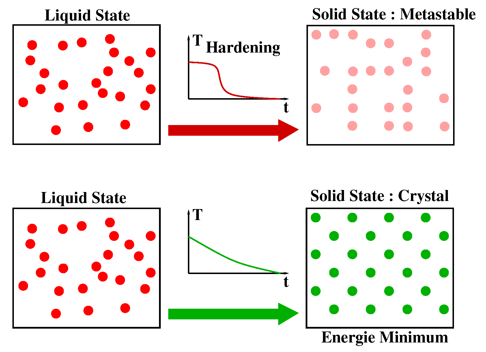
4.1. Standard Simulated Annealing
- Bring the solid to a very high temperature until “melting” of the structure;
- Cool the solid according to a particular temperature decreasing scheme in order to reach a solid-state of minimum energy.

- The state-space points represent the possible states of the solid;
- The function to be minimized represents the energy of the solid.
- 1
- Initialization (, , , );
- 2
- Repeat:
- 3
- For to do
- Generate a solution j from the neighborhood of the current solution i;
- If then (j becomes the current solution);
- Else, j becomes the current solution with probability ;
- 4
- ;
- 5
- Compute();
- 6
- Until ;
4.2. Evaluation-Based Simulation
- 1
- The new solution is accepted and, in this case, only the current objective-function value is updated.
- 2
- Else, the comeback operator is applied to the current position in the state space in order to come back to the previous solution before the generation, again without any duplication in the memory.
4.3. Selective Simulated Annealing (SSA)
4.4. Implementation of SSA for Our Problem
4.4.1. Coding of the Solution
4.4.2. Neighboring Operator
4.4.3. Objective Function Computation
5. Results
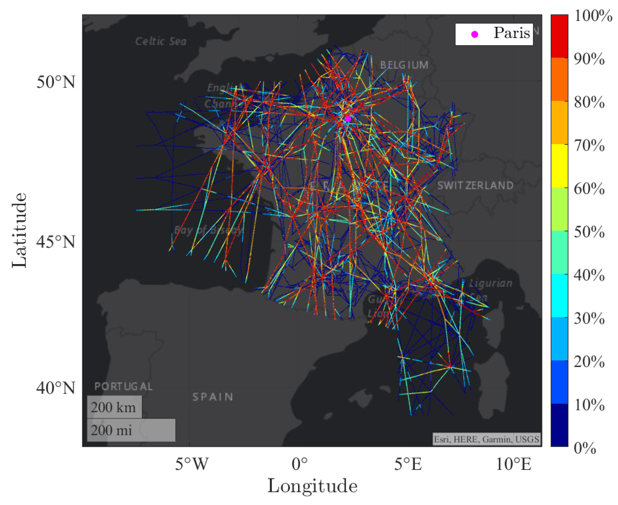
5.1. Benchmark Data
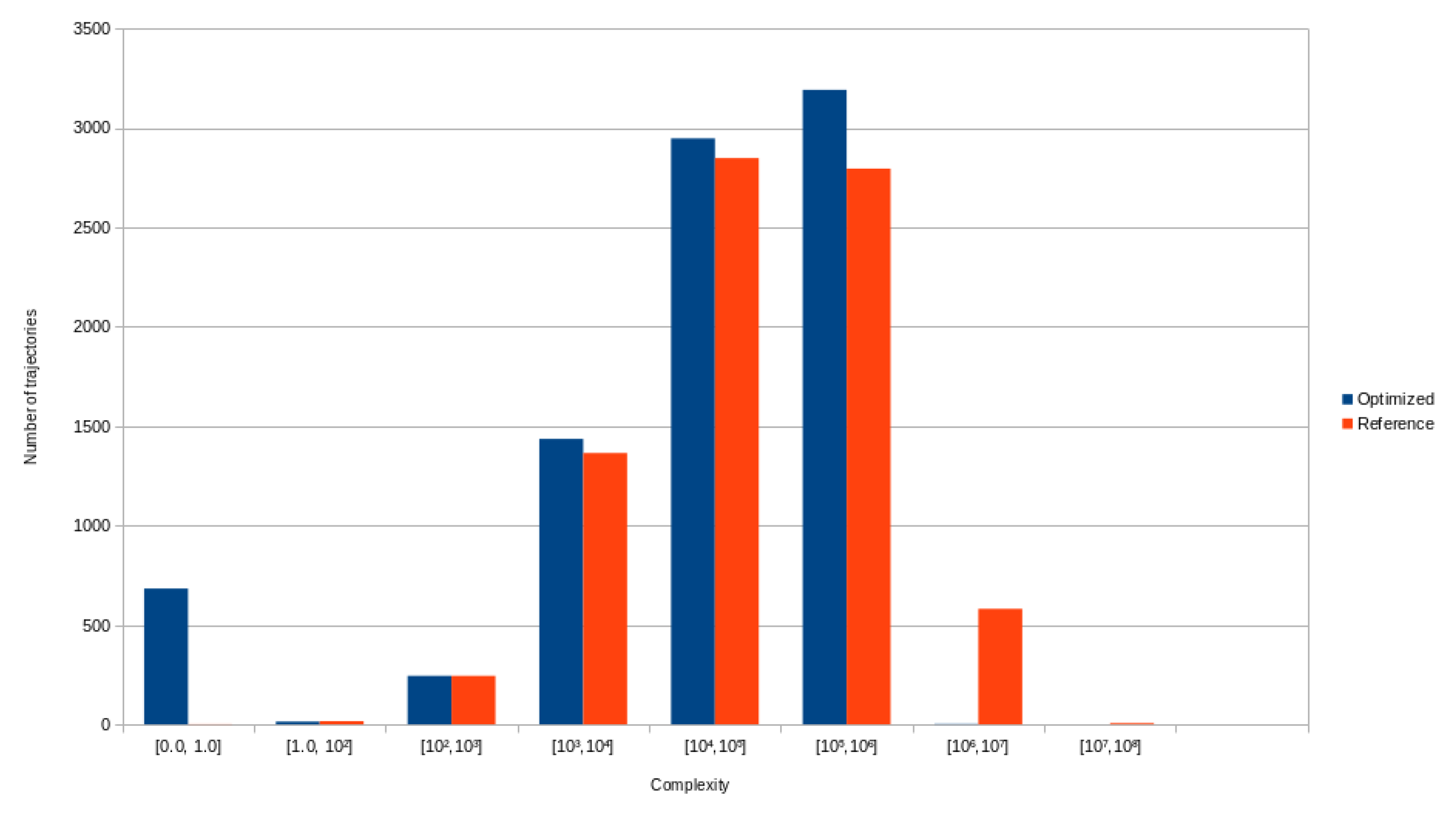
5.2. Benchmark Results
- CPU: Intel Xeon Gold 6230 at 2.10 Ghz;
- RAM: 1 TB.
6. Conclusions
Author Contributions
Funding
Institutional Review Board Statement
Informed Consent Statement
Conflicts of Interest
References
- Hilburn, B. Cognitive Complexity and Air Traffic Control: A Literature Review; Technical Report; Center for Human Performance: Soesterberg, The Netherland, 2004. [Google Scholar]
- Mogford, H.; Guttman, J.; Morrowand, P.; Kopardekar, P. The Complexity Construct in Air Traffic Control: A Review and Synthesis of the Literature; Technical Report; FAA: Atlantic City, NJ, USA, 1995.
- Durand, N.; Gotteland, J.B. Genetic algorithms applied to air traffic management. In Metaheuristics for Hard Optimization: Simulated Annealing, Tabu Search, Evolutionary and Genetic Algorithms, Ant Colonies, … Methods and Case Studies; Dréo, J., Siarry, P., Pétrowski, A., Taillard, E., Eds.; Springer: Berlin/Heidelberg, Germany, 2006; pp. 277–306. [Google Scholar]
- Barnier, N.; Allignol, C. 4D-Trajectory Deconfliction through Departure Time Adjustment; Eighth USA/Europe Air Traffic Management Research and Development Seminar: Napa, CA, USA, 2009. [Google Scholar]
- Barnier, N.; Allignol, C. Combining Flight Level Allocation with Ground Holding to Optimize 4D-Deconfliction; Ninth USA/Europe Air Traffic Management Research and Development Seminar: Berlin, Germany, 2011. [Google Scholar]
- Dougui, N.; Delahaye, D.; Puechmorel, S.; Mongeau, M. A New Method for Generating Optimal Conflict Free 4D Trajectory. In Proceedings of the 4th International Conference on Research in Air Transportation, Budapest, Hungary, 1–4 June 2010. [Google Scholar]
- Dougui, N.; Delahaye, D.; Puechmorel, S.; Mongeau, M. A light-propagation model for aircraft trajectory planning. J. Glob. Optim. 2013, 56, 873–895. [Google Scholar] [CrossRef]
- Islami, A.; Chaimatanan, S.; Delahaye, D. Large scale 4D trajectory planning. In Air Traffic Management and Systems—II; Lecture Notes in Electrical Engineering; Springer: Tokyo, Japan, 2016; Volume 420, pp. 27–47. [Google Scholar]
- Odoni, A. The flow management problem in air traffic control. In Flow Control of Cogested Networks; Odoni, A.E.A., Ed.; NATO ASI Series; Springer: Berlin/Heidelberg, Germany, 1987; Volume F38, pp. 269–288. [Google Scholar]
- Terrab, M.; Odoni, A. Strategic Flow Management for Air Traffic Control. Oper. Res. 1993, 41, 138–152. [Google Scholar] [CrossRef]
- Richetta, O.; Odoni, A. Dynamic Solution to the Ground-Holding Problem in Air Traffic Control. Transp. Res. 1994, 28, 167–185. [Google Scholar] [CrossRef]
- Andreatta, G.; Romanin-Jacur, G. Aircraft Flow Management under Congestion. Transp. Sci. 1987, 21, 249–253. [Google Scholar] [CrossRef]
- Richetta, O.; Odoni, A. Solving Optimally the Static Ground Holding Policy Problem in Air Traffic Control. Transp. Sci. 1993, 27, 228–238. [Google Scholar] [CrossRef]
- Wang, H. A Dynamic Programming Framework for the Global Flow Control Problem in Air Traffic Management. Transp. Sci. 1991, 25, 308–313. [Google Scholar] [CrossRef][Green Version]
- Andreatta, G.; Odoni, A.; Richetta, O. Models for the ground holding problem. In Large Scale Computation and Information Processing in Air Traffic Control; Bianco, L., Odoni, A., Eds.; Transportation Analysis; Springer: Berlin/Heidelberg, Germany, 1993; pp. 125–168. [Google Scholar]
- Bertsimas, D.; Stock, S. The Air Traffic Flow Management Problem with En-Route Capacities; Technical Report; A.P Sloan School of Management. M.I.T.: Cambridge, MA, USA, 1994. [Google Scholar]
- Tosic, V.; Babic, O.; Cangalovic, M.; Hohlacov, D. Some models and algorithms for en-route air traffic flow management faculty transport. Transp. Plan. Technol. 1995, 19, 147–164. [Google Scholar] [CrossRef]
- Alam, S.; Delahaye, D.; Chaimatanan, S.; Féron, E. A distributed air traffic flow management model for european functional airspace blocks. In Proceedings of the 12th USA/Europe Air Traffic Management Research and Development Seminar, Seattle, WA, USA, 27–30 June 2017. [Google Scholar]
- Juntama, P.; Chaimatanan, S.; Alam, S.; Delahaye, D. A distributed metaheuristic approach for complexity reduction in air traffic for strategic 4D trajectory optimization. In Proceedings of the AIDA-AT 2020, 1st Conference on Artificial Intelligence and Data Analytics in Air Transportation, Singapore, 3–4 February 2020; pp. 1–9, ISBN 978-1-7281-5381-0. [Google Scholar]
- Kirkpatrick, S.; Gelatt, C.; Vecchi, M. Optimization by simulated annealing. Science 1983, 220, 671–680. [Google Scholar] [CrossRef] [PubMed]
- Metropolis, N.; Rosenbluth, A.; Rosenbluth, M.; Teller, A.; Teller, E. Equation of state calculation by fast computing machines. J. Chem. Phys. 1953, 21, 1087–1092. [Google Scholar] [CrossRef]
- Chaimatanan, S.; Delahaye, D.; Mongeau, M. Strategic deconfliction of aircraft trajectories. In Proceedings of the ISIATM 2013, the 2nd International Conference on Interdisciplinary Science for Innovative Air Traffic Management, Toulouse, France, 8–10 July 2013. [Google Scholar]
- Chaimatanan, S.; Delahaye, D.; Mongeau, M. A hybrid metaheuristic optimizationalgorithm for strategic planning of 4D aircraft trajectories at the continental scale. Comput. Intell. Mag. 2014, 9, 46–61. [Google Scholar] [CrossRef]


| Number of Flights | Initial Worst Congestion | Final Worst Congestion | Computation Time | |
|---|---|---|---|---|
| Time shifting | 8800 | 1,500,000 | 120,000 | 7700 (2 h) |
Publisher’s Note: MDPI stays neutral with regard to jurisdictional claims in published maps and institutional affiliations. |
© 2021 by the authors. Licensee MDPI, Basel, Switzerland. This article is an open access article distributed under the terms and conditions of the Creative Commons Attribution (CC BY) license (https://creativecommons.org/licenses/by/4.0/).
Share and Cite
Lavandier, J.; Islami, A.; Delahaye, D.; Chaimatanan, S.; Abecassis, A. Selective Simulated Annealing for Large Scale Airspace Congestion Mitigation. Aerospace 2021, 8, 288. https://doi.org/10.3390/aerospace8100288
Lavandier J, Islami A, Delahaye D, Chaimatanan S, Abecassis A. Selective Simulated Annealing for Large Scale Airspace Congestion Mitigation. Aerospace. 2021; 8(10):288. https://doi.org/10.3390/aerospace8100288
Chicago/Turabian StyleLavandier, Julien, Arianit Islami, Daniel Delahaye, Supatcha Chaimatanan, and Amir Abecassis. 2021. "Selective Simulated Annealing for Large Scale Airspace Congestion Mitigation" Aerospace 8, no. 10: 288. https://doi.org/10.3390/aerospace8100288
APA StyleLavandier, J., Islami, A., Delahaye, D., Chaimatanan, S., & Abecassis, A. (2021). Selective Simulated Annealing for Large Scale Airspace Congestion Mitigation. Aerospace, 8(10), 288. https://doi.org/10.3390/aerospace8100288