A Method for Improved Flight Testing of Remotely Piloted Aircraft Using Multisine Inputs

Abstract

Unless a segregated airspace and the corresponding clearances can be afforded, flight testing of remotely piloted aircraft is often done near the ground and within visual line-of-sight. In addition to the increased exposure to turbulence, this setup also limits the available time for test manoeuvres on each pass, especially for subscale demonstrators with a relatively high wing loading and flight speed. A suitable testing procedure, efficient excitation signals and a robust system identification method are therefore fundamental. Here, the authors use ground-based flight control augmentation to inject multisine signals with low correlation between the different inputs. Focusing on initial flight-envelope expansion, where linear regression is common, this paper also describes the improvement of an existing frequency-domain method by using an instrumental variable (IV) approach to better handle turbulence and measurement noise and to enable real-time identification analysis. Both simulations and real flight tests on a subscale demonstrator are presented. The results show that the combination of multisine input signals and the enhanced frequency-domain method is an effective way of improving flight testing of remotely piloted aircraft in confined airspace.

1. Introduction

Systematic flight testing of remotely piloted aircraft (RPA) is usually done in two different situations: One is the development of the platform itself for its use as a final product, as in the case of unmanned aerial systems (UASs). The second is during the early investigation and development of a particular configuration, feature or technology that is intended to be part of a larger, often manned, system. In this second case, typically referred to as scaled or subscale flight testing (SFT), RPAs are carefully designed to reproduce certain characteristics of the full-scale system [1,2]. During the early stages of design or technology development, SFT can be used to increase the available knowledge in a relevant environment without the high cost and risk associated with full-scale flight testing [2,3,4]. An example of an early use of this technique is shown in Figure 1.

One of the potential areas of interest for SFT is the investigation of flight dynamics. The complexity of modern aircraft design requires both the static and dynamic flight-mechanical characteristics of the aircraft to get a full picture of the expected performance. Historically, wind-tunnel testing has been the main source of aerodynamic knowledge for aircraft design [5]. Currently, the static aircraft characteristics can be evaluated more easily and earlier in the design thanks to the continuous increase of computational power and the advances in computational fluid dynamic (CFD) methods. However, reliable dynamic characteristics are still difficult to obtain and evaluate or they become only available at later stages of detailed design. This makes SFT an interesting and affordable method to reduce uncertainty: the stability and control characteristics of the full-scale aircraft can be assessed with a dynamically scaled model, as described in [1,2,6,7].

Flight testing a remotely piloted aircraft can in some cases require a costly infrastructure with robust and reliable ground support for the flight crew and the test team, as described in [8]. 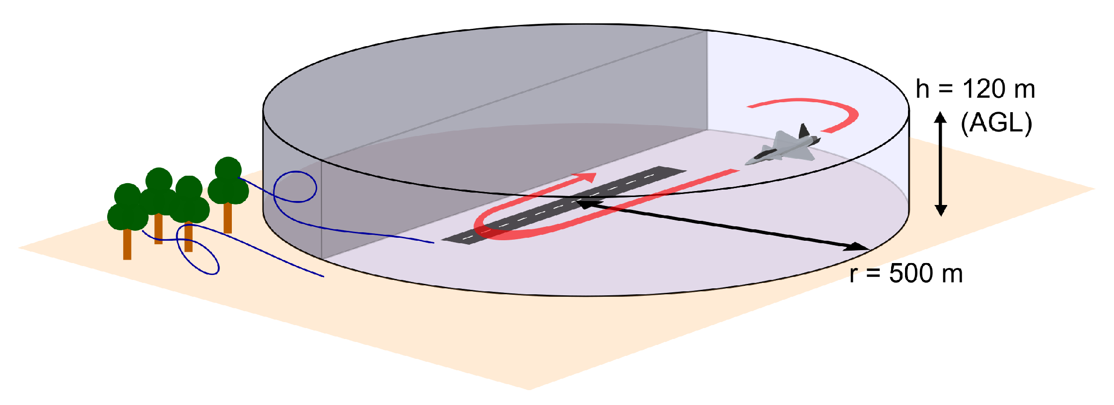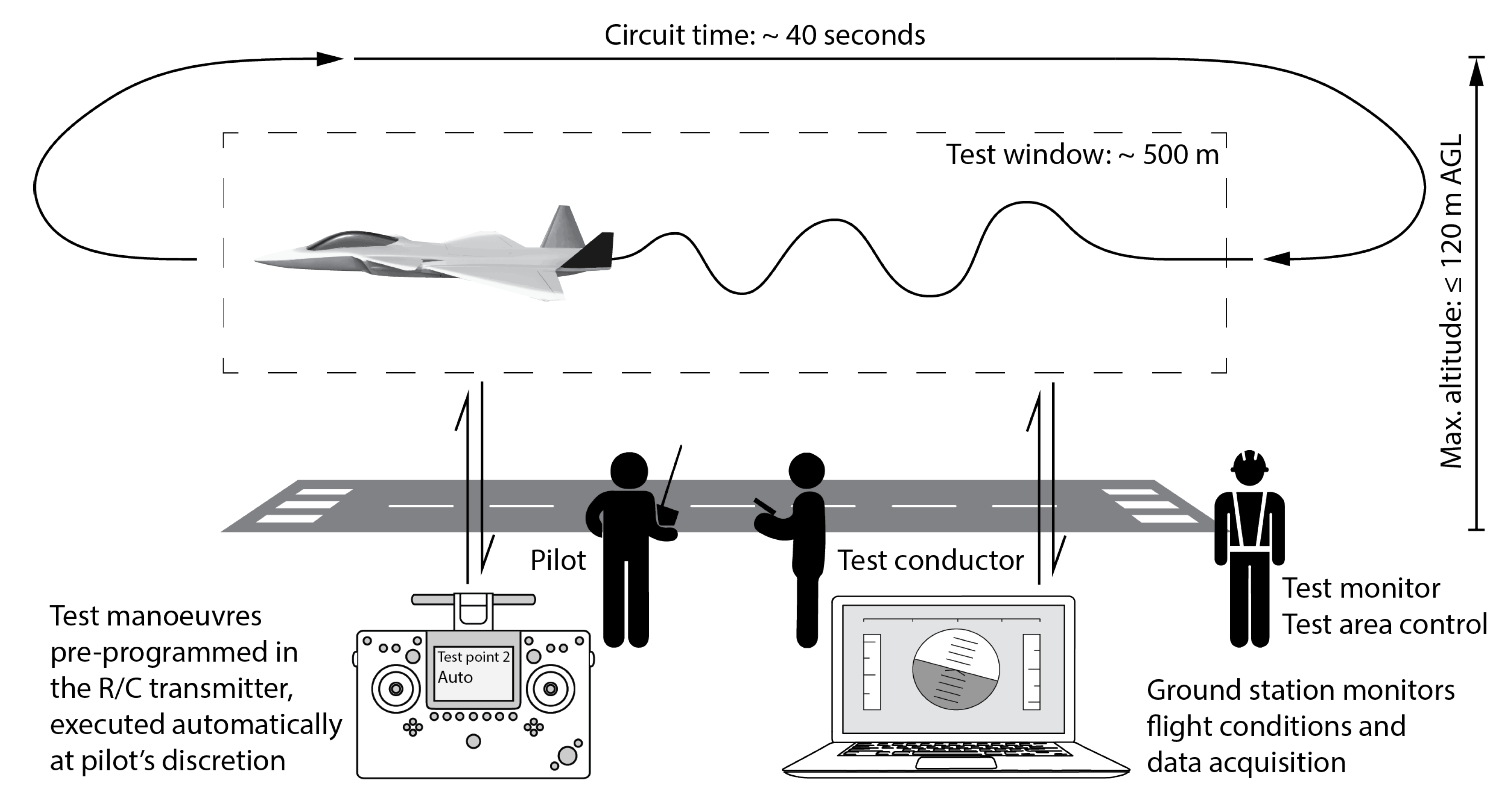Fortunately, modern developments in consumer radio-controlled (RC) systems and UAS equipment have enabled smaller organizations to perform relatively advanced flight tests with less resources and in shorter times [9]. Due to the current regulations in most countries and unless a segregated airspace and the corresponding clearances can be afforded, the flight test is likely to take place at low altitude and within the visual line-of-sight (VLOS). While this type of operation is more economical, it presents two main challenges represented in Figure 2: First, subscale demonstrators often have a high wing loading and fly faster than typical RC aircraft, leaving little time for test manoeuvres on each pass. Second, the aircraft is exposed to higher levels of turbulence near the ground. An illustrative example of the consequences of VLOS limitations for subscale experiment design is the recent FLEXOP project: even the test-bed aircraft was specifically designed to cope with the fast transitions needed to reach the desired flight condition within the designated test perimeter [10].

The methods presented in this paper aim to improve both the productivity of the flight test and the quality of the modelling under these demanding circumstances. The focus is mainly on the initial flight envelope expansion, where usually, linear flight-mechanical characteristics are studied and primary flying qualities are compared to the existing models. At this stage, test manoeuvres typically involve relatively small disturbances from trimmed states. Single, double (doublets) or multiple pulses are some of the control inputs traditionally used for excitation in both open- and closed-loop systems.

Here, the application of multisine input signals for system excitation is proposed. Compared to classical pulses, multisine input signals enable simultaneous excitations of different control surfaces, and hence, they have the potential to maximise the information obtained during a very short time. Although uncommon in full-scale aircraft testing, this type of input signal was tested on NASA’s T-2 subscale jet transport aircraft in 2012 [11]. While NASA’s T-2 is comparable in terms of size, flight speed and instrumentation to the aircraft tested here, the testing environment is relatively more demanding here due to VLOS operation.

The means for dealing with air turbulence, especially noticeable near the ground, also need to be considered. There are aircraft parameter estimation algorithms for system identification that take process and measurement noise into account, as described in [12]. However, the problem formulation in this paper is of an errors-in-variable character. An instrumental variable (IV) approach is a common way of dealing with this type of problem. An algorithm using this approach was given in [13]. This approach is used to improve the algorithm performance.

An additional issue when using SFT at an early stage of design is that only basic knowledge of the aircraft characteristics may be available by the start of the campaign. It can therefore be helpful to use online tools for monitoring the information acquired during flight in real time. One such interesting method for the estimation of the flight mechanical parameters was given by Morelli [14]. This method is based on a frequency domain approach, which is fast and suitable for real-time applications. It can also be used to make decisions about the continuation or interruption of the testing if anything deviates from the expected conditions.

The methods proposed here are described in Section 2. These were also tested on a real flight experiment using a jet-powered subscale aircraft denominated the Generic Future Fighter (GFF) demonstrator [15]. The multisine input signals were designed by using a simulation model based on basic data from earlier flights [16]. The results of the input design are presented in Section 3, and the details of the experiment and its results are presented in Section 4, Section 5 and Section 6. Conclusions are presented in Section 7.

2. Methods

A state-space representation of a linear time-invariant system can be written as:

$$\dot{x}(t)=Ax(t)+Bu(t)+w(t)$$

(1a)

$$y(t)=Cx(t)+Du(t)+v(t)$$

(1b)

where $x(t)$ is an $n\times 1$ state vector, $u(t)$ is an $m\times 1$ input vector and $w(t)$ is the system noise, which in the current application corresponds to turbulence. This cannot be assumed to be white. Furthermore, $y(t)$ is a $p\times 1$ output, and $v(t)$ is measurement noise, which is here assumed to be zero mean white noise with covariance R. For the output, it is assumed that $C=I$ and $D=0$.

2.1. Original Method

The basics of the original method, used in this paper, come from the work in [14]. This is a method for estimating continuous-time flight mechanical parameters in the matrices A and B in (1a). The method consists of two parts, which for the convenience of the reader are repeated in brief below.

2.1.1. Sequential Fourier Transform

For a finite time interval, the continuous-time Fourier transform is defined by:

$${\tilde{f}}_T({\omega }_i)\equiv {\int }_0^{T}f(t)e^{-j{\omega }_{i}t}dt$$

(2)

where $\tilde{}$ is used to denote the transformed entities and ${\omega }_i$ is the frequency of interest.

When data are sampled, a rectangle approximation of the integral of the finite Fourier transform with a sampling time $T_s$ can be used:

$${\tilde{f}}_T({\omega }_i)\approx T_s\sum _{k=0}^{N-1}{f}_k{e}^{-j{\omega }_{i}k{T}_s}=T_s{\tilde{F}}_N({\omega }_i)$$

(3)

where $t\equiv k{T}_s$, $f_k\equiv f(k{T}_s)$ and ${\tilde{F}}_N({\omega }_i)$ is the discrete Fourier transform at time T. This will give a reasonable approximation if the sample time $T_s$ is short relative to changes in $f(t)$.

The discrete Fourier transform can be updated sequentially as the number of samples, N, increases. At time $t=N{T}_s$, this becomes:

$$\begin{array}{cc}\hfill {\tilde{F}}_N({\omega }_i)& ={\tilde{F}}_{N-1}({\omega }_i)+f_{N-1}{e}^{-j{\omega }_i(N-1)T_s}\hfill \end{array}$$

(4)

For the transformation of a time derivative:

$${\tilde{\dot{F}}}_N({\omega }_i)=j{\omega }_i{\tilde{F}}_N({\omega }_i)+f_N{e}^{-j{\omega }_{i}N{T}_s}-f_0$$

(5)

has to be used to get the correct implementation. The effect of the boundary terms $f_N$ and $f_0$ was analysed in [13].

2.1.2. Complex Least Squares Regression

Transforming the input and measurement signals in (1a) and using the measurements from (1b), with $C=I$ and $D=0$, as an approximation of the states give:

$$\begin{array}{c}\hfill j{\omega }_i{\tilde{Y}}_N^T+y_N^T{e}^{-j{\omega }_{i}N{T}_s}-y_0^T=\left[\begin{array}{cc}{\tilde{Y}}_N^T& {\tilde{U}}_N^T\end{array}\right]{\left[\begin{array}{cc}A& B\end{array}\right]}^T+{\tilde{V}}_N^T\end{array}$$

(6)

where ${\tilde{V}}^T$ contains the combined noise terms from $v(t)$ and $w(t)$. When analysing (6) using M frequencies, this equation becomes a linear regression of the form:

$$\tilde{z}(\omega )=\tilde{\Phi }(\omega )\theta +{\tilde{V}}^T(\omega )$$

(7)

where $\omega$ now is an $M\times 1$ vector. Furthermore, $\tilde{z}$ is an $M\times n$ matrix, and $\tilde{\Phi }$ is an $M\times (n+m)$ matrix containing the regressors. The $(n+m)\times n$ matrix $\theta ={\left[AB\right]}^T$ includes the system parameters in A and B to be estimated, and ${\tilde{V}}^T(\omega )$ is an $M\times n$ noise matrix.

Morelli [14] proposed that the parameter estimation in the linear regression (7) should be solved with a complex least squares (CLS) method where the prediction error is given as:

$$\tilde{\epsilon }(\omega ,\theta )=\tilde{z}(\omega )-\tilde{\Phi }(\omega )\theta$$

(8)

The CLS criterion then becomes:

$$V_M(\theta ,Z^M)=\frac{1}{2}(\tilde{z}-\tilde{\Phi }\theta )\ast (\tilde{z}-\tilde{\Phi }\theta )$$

(9)

where ∗ is the complex conjugate transpose. This gives the parameter estimator:

$$\widehat{\theta }={(Re(\tilde{\Phi }\ast \tilde{\Phi }))}^{-1}Re(\tilde{\Phi }\ast \tilde{z}).$$

(10)

The estimated parameter covariance is given as:

$${\widehat{P}}_k={\widehat{\sigma }}_k^{2}Re{(\tilde{\Phi }\ast \tilde{\Phi })}^{-1}$$

(11)

where k is a column index of $\theta$. Here, the estimated error variance ${\sigma }_k^2$ is given by:

$${\widehat{\sigma }}_k^2=\frac{1}{M-n_p}(({\tilde{z}}_k-\tilde{\Phi }{\widehat{\theta }}_k)\ast ({\tilde{z}}_k-\tilde{\Phi }{\widehat{\theta }}_k))$$

(12)

where $n_p$ is the number of parameters to be estimated for each column k. The estimated parameter uncertainties are two standard deviations. The estimated standard deviation is given by:

$${\widehat{s}}_{k,i}=\sqrt{{\widehat{P}}_{k,ii}(\widehat{\theta })},i=1,...,n_p$$

(13)

The expression for the covariance matrix in (11) shows why a careful experiment design is crucial for the estimator performance. Datasets where there is a high correlation between several regressors will make the covariance matrix ill-conditioned and reduce the estimator accuracy. Hence, the experiments should preferably be designed such that this problem is avoided as much as possible.

2.2. Suggested Improvement

A suggested improvement is introduced to handle noisy data coming from both measurement and process noise. Typically, the noise ${\tilde{V}}_N$ has to be white and uncorrelated with the regressors in $\tilde{\Phi }$ for the original method to be consistent. This cannot be guaranteed in the RC tests described in this paper.

Instrumental Variables

In a real flight, the process noise comes from non-white turbulence, which affects the regressors. This might lead to biased estimates. To take care of the bias effect, the use of a complex instrumental variable (CIV) approach was suggested in [13], where the resulting effect was shown mainly for simulations. Suitable instruments $\tilde{\zeta }$, which are uncorrelated with the true process noise ${\tilde{V}}_0$, but correlated with the regressors, have to be chosen. This will, according to [17], give the new parameter estimate:

$$\widehat{\theta }={(Re(\tilde{\zeta }\ast \tilde{\Phi }))}^{-1}Re(\tilde{\zeta }\ast \tilde{z})$$

(14)

and the covariance expression:

$${\widehat{P}}_k(\widehat{\theta })={\widehat{\sigma }}_k^{2}Re{(\tilde{\zeta }\ast \tilde{\Phi })}^{-1}Re(\tilde{\zeta }\ast \tilde{\zeta })Re{(\tilde{\Phi }\ast \tilde{\zeta })}^{-1}$$

(15)

The estimated error variance and parameter standard deviation have the same forms as in (12) and (13).

Adding the suggested improvements to the original method gives the new method to be used.

3. Input Design Using Simulated Data

This section describes the design of input signals applied during the practical experiment on the Generic Future Fighter (GFF) subscale aircraft. First, a linear state-space simulation model was created based on the data available from previous flights of this aircraft [16]. This model takes the form:

$$\begin{array}{cc}\hfill & \left[\begin{array}{c}\dot{\alpha }(t)\\ \dot{q}(t)\end{array}\right]=\left[\begin{array}{cc}{Z}_{\alpha }& Z_q\\ M_{\alpha }& M_q\end{array}\right]\left[\begin{array}{c}\alpha (t)\\ q(t)\end{array}\right]+\left[\begin{array}{cc}{Z}_{{\delta }_e}& Z_{{\delta }_c}\\ M_{{\delta }_e}& M_{{\delta }_c}\end{array}\right]\left[\begin{array}{c}{\delta }_e(t)\\ {\delta }_c(t)\end{array}\right]\hfill \\ \hfill & \left[\begin{array}{c}{\alpha }_m(t)\\ q_m(t)\end{array}\right]=\left[\begin{array}{cc}1& 0\\ 0& 1\end{array}\right]\left[\begin{array}{c}\alpha (t)\\ q(t)\end{array}\right]\hfill \end{array}$$

(16)

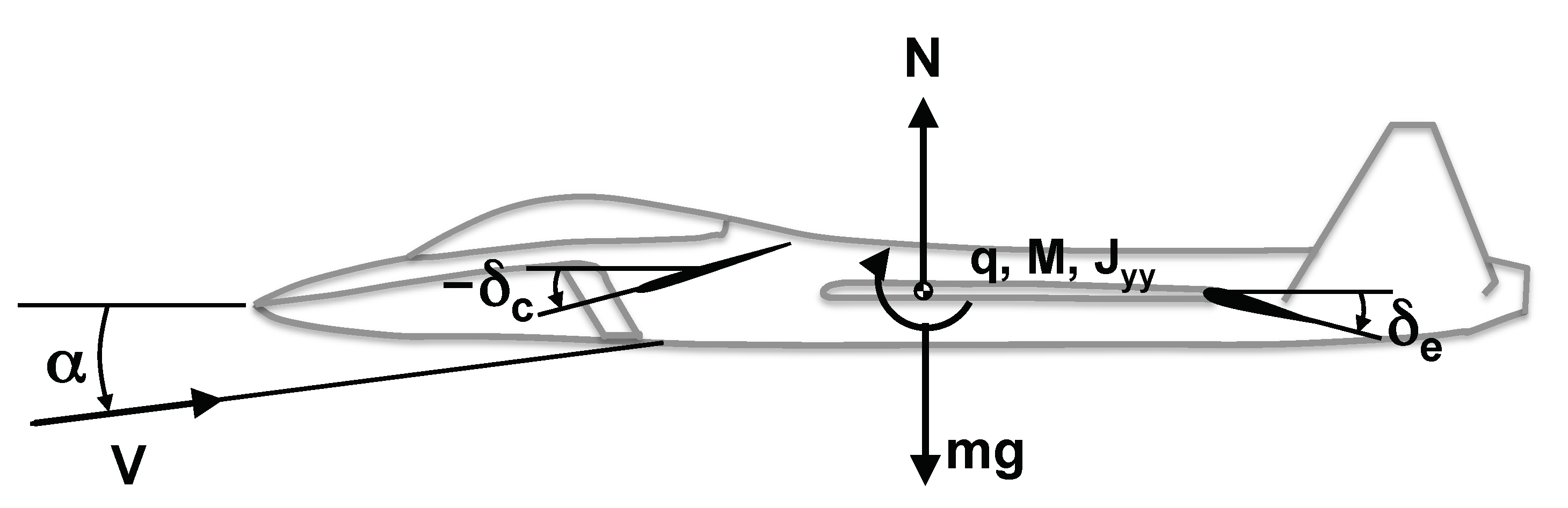
where the considered variables are defined in Figure 3.

The states $x(t)={\left[\begin{array}{cc}\alpha (t)& q(t)\end{array}\right]}^T$ are the angle-of-attack and the pitch rate, and the input $u(t)={\left[\begin{array}{cc}{\delta }_e(t)& {\delta }_c(t)\end{array}\right]}^T$ consists of the elevator and canard deflections. All states are measured.

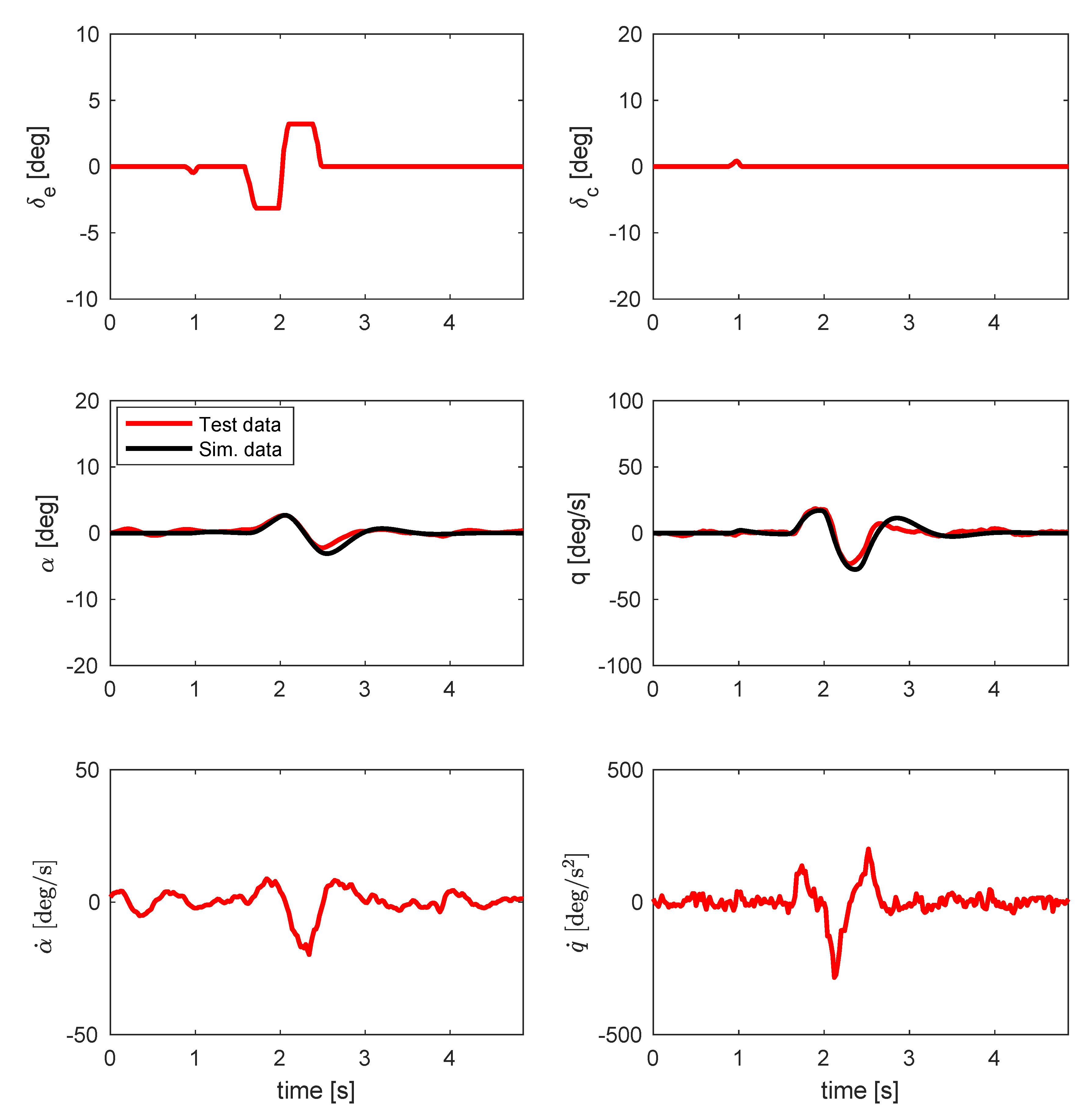
Making an estimation of the model parameters Z and M in (16) using an ordinary least squares (OLS) time domain method [17] on the existing data shown in Figure 4 leads to the following continuous-time model:

$$\begin{array}{cc}\hfill \dot{x}(t)& =\left[\begin{array}{cc}-1.88& 0.65\\ -36.39& -2.77\end{array}\right]x(t)+\left[\begin{array}{cc}-0.33& -0.37\\ -39.04& 17.49\end{array}\right]u(t)\hfill \\ \hfill y(t)& =\left[\begin{array}{cc}1.00& 0.00\\ 0.00& 1.00\end{array}\right]x(t)\hfill \end{array}$$

(17)

The OLS in the time domain is used here in batch mode since the whole dataset is available, and it is a quick and easy way to get a model to use. The model (17) was validated on other datasets. One of these is shown in Figure 5. Even though the match was not perfect, the model was deemed accurate enough to be used for the experimental design.

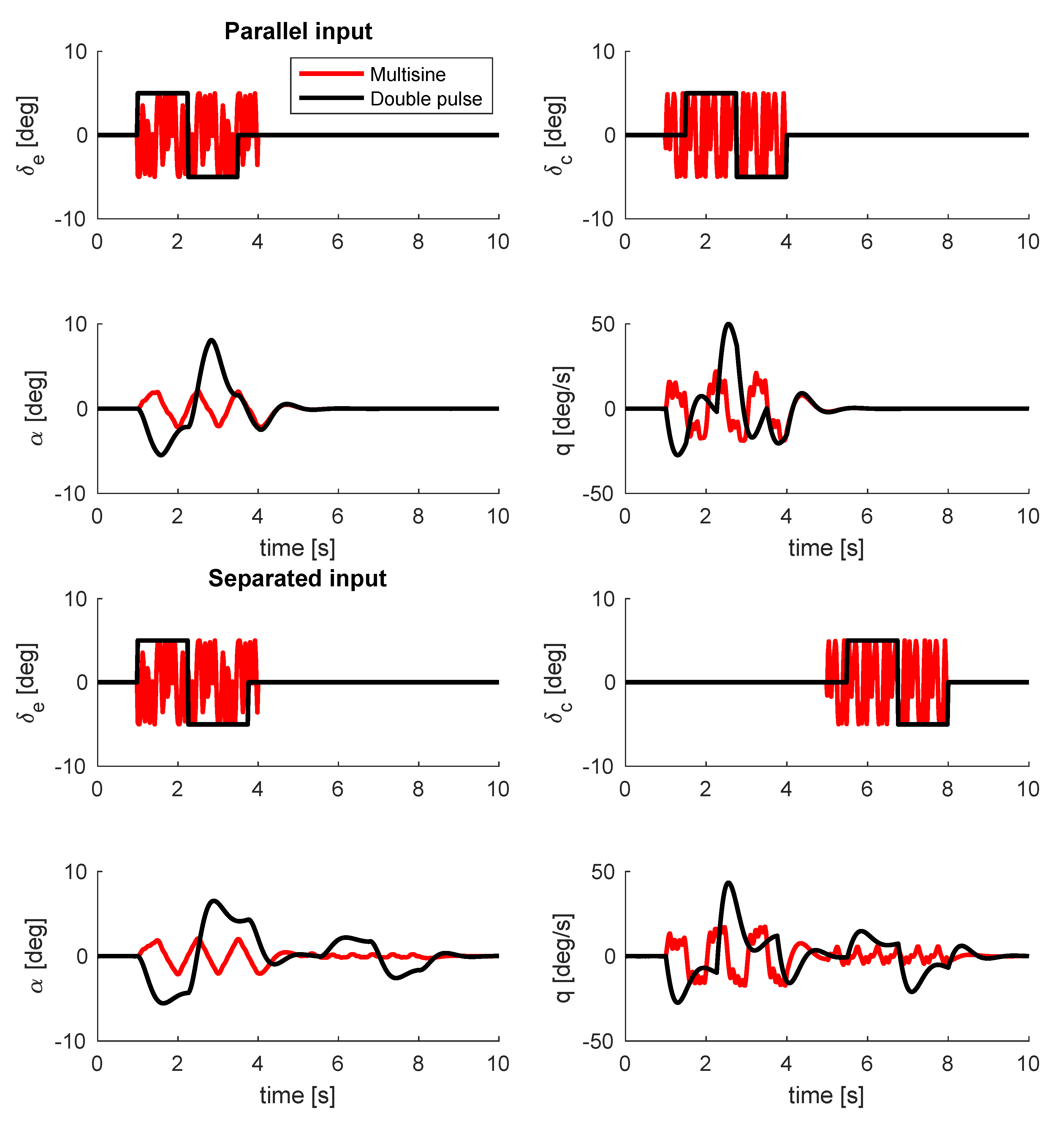
Two types of signals were evaluated (see Figure 6). The first one is a double pulse, commonly used for estimating aerodynamic derivatives from flight test data. The second one is a multisine signal:

$$\begin{array}{c}\hfill u(t)=\sum _{r=1}^{N_u}{A}_{r}cos({\omega }_{0}rt+{\phi }_r)\end{array}$$

(18)

where $A_r$ and ${\phi }_r$ are the amplitudes and phases of the signal components, respectively. One reason for using a multisine is that it is possible to achieve weakly correlated, simultaneously excited input signals by using different frequencies for the different control surfaces, a method described in [11]. This will save time and reduce cost since it reduces the time spent in the air for the same amount of information gathered.

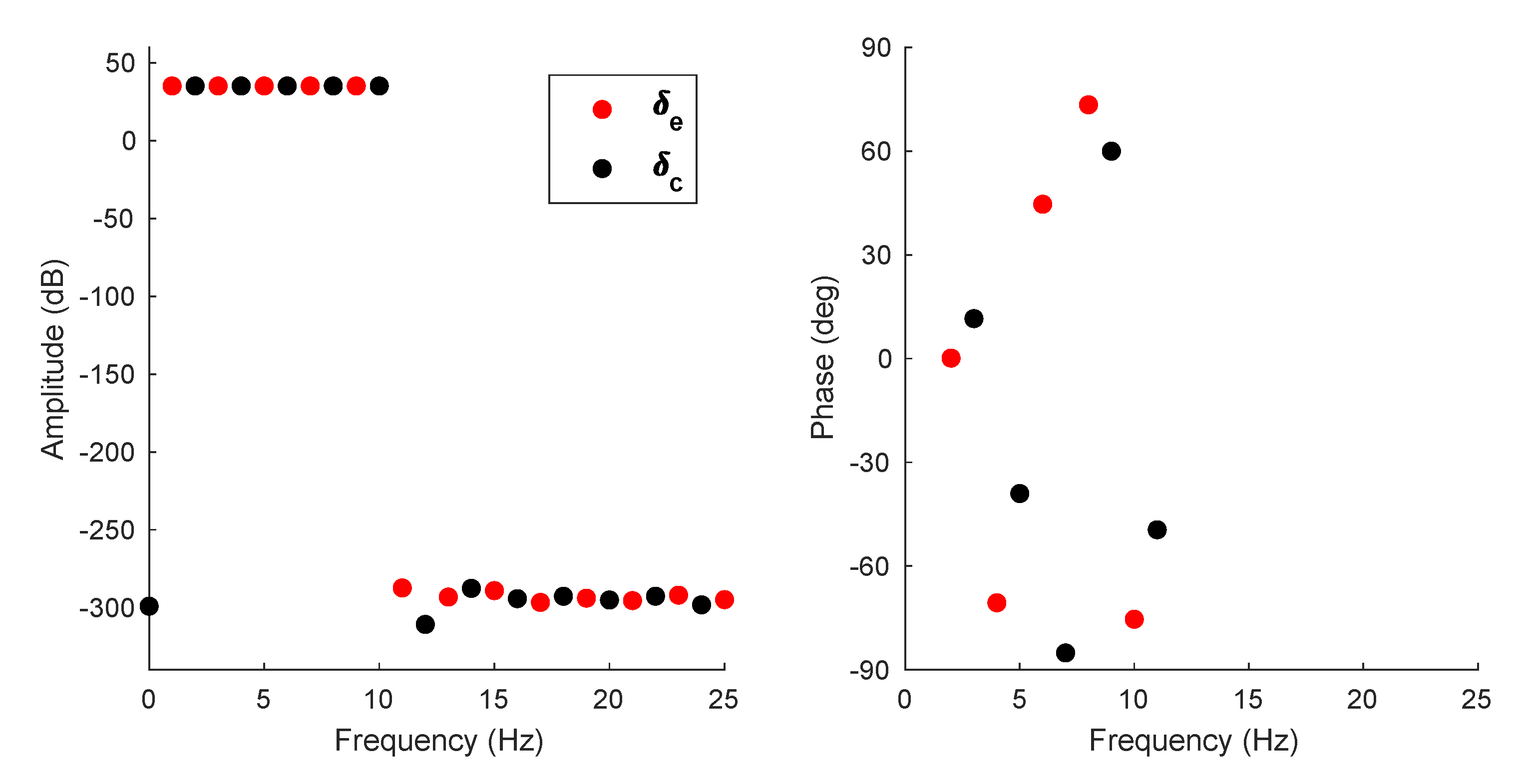
Nine different crest factor multisine input signals were created with a sample frequency of $100$ Hz and a period of $1$s. The toolbox described in [18] was used to generate the crest factor optimized input signals. An example of the amplitudes and the phases of the separated input signals is shown in Figure 7, where the phases corresponding to low-amplitude frequencies are omitted.

Three periods of excitation were used to get good input signals: one to take care of the transient in the beginning and two steady-state periods. This type of signal was described in [19], where it was used to detect non-linearities.

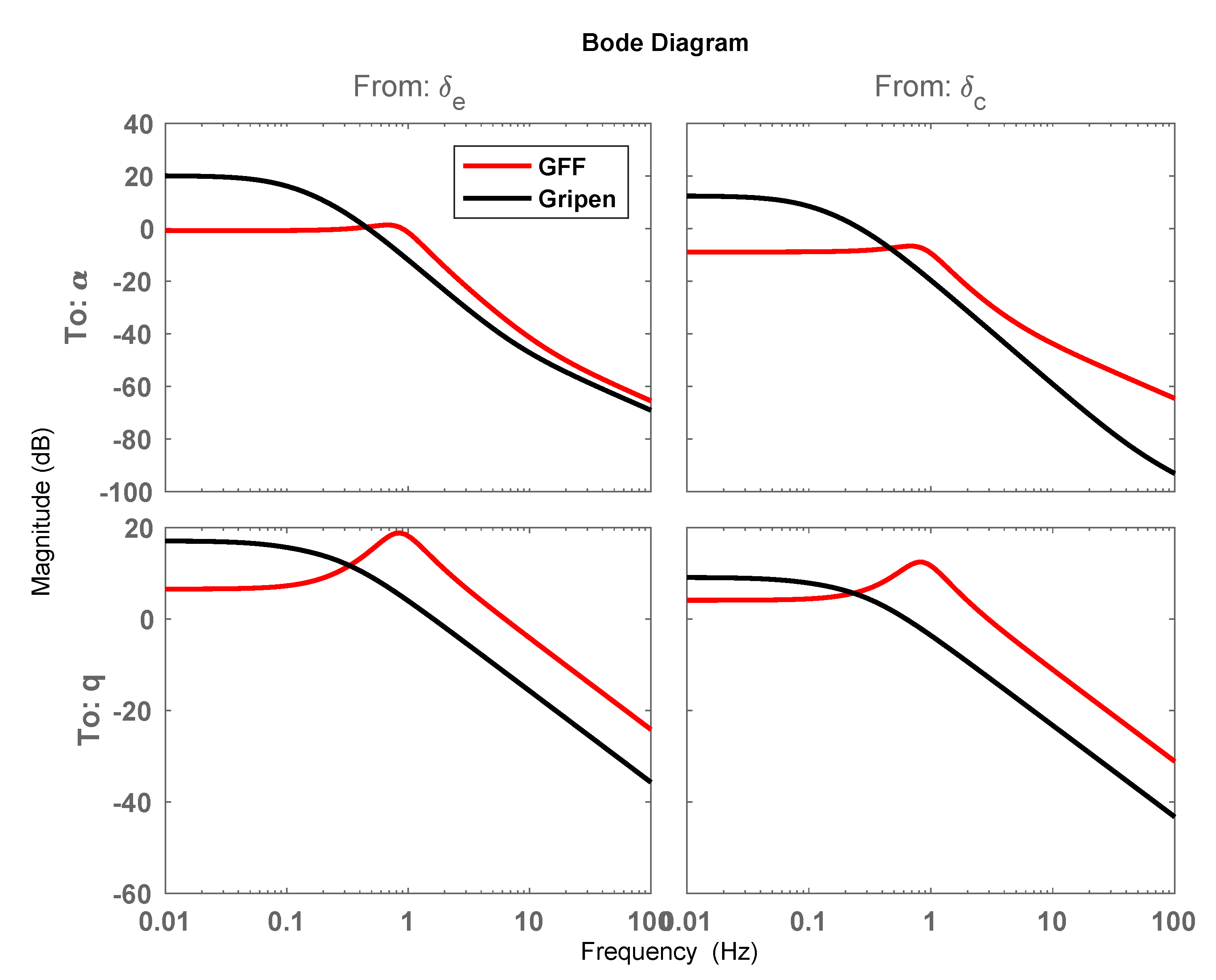
Note that the frequency span of 1–10 Hz was chosen to excite the short period flight-mechanical model for the GFF subscale demonstrator. This is higher than the 0.1–2 Hz typically used for full-sized aircraft as in [14]. It is a well known fact that small-scale aircraft have this short period characteristic. This phenomenon can be seen in the Bode plot of Figure 8, where the model of a full-scale Saab JAS 39 Gripen used in [13] is compared to the subscale GFF model from (17).

To investigate the possible benefits of the multisine signals, the inputs for the elevator and the canard will be run both separately and in parallel. They will also be compared to the double pulse input when separated and with a small time delay to mimic the parallel input without causing too much correlation between the different control surfaces. Examples of input signals from simulations, with a process noise of about ten percent of the input amplitude, are shown in Figure 9. The total excitation time here is $10$s, which is the expected time window available in the real flight test.

Making simulations with the estimated models for nine realisations of the input signals and comparing the double pulse (DP) and the crest factor optimized multisine (MS) results to the true model using the relative error:

$$\epsilon =100|\frac{{\theta }_{model}-{\theta }_{true}}{{\theta }_{true}}|$$

(19)

as a measure give the results in

Table 1. The relative error (19) when using the double pulse (DP) and the crest factor optimized multisine (MS) input signals. The true model (17) is given as a reference.

	True Model	${\mathit{\epsilon }}_{\mathit{DP}}$	${\mathit{\epsilon }}_{\mathit{MS}}$
$Z_{\alpha }$	$-1.880$	$1.601$	$0.997$
$Z_q$	$0.651$	$0.868$	$0.386$
$Z_{{\delta }_e}$	$-0.332$	$3.703$	$2.871$
$Z_{{\delta }_c}$	$-0.367$	$10.430$	$0.619$
$M_{\alpha }$	$-36.395$	$0.829$	$0.514$
$M_q$	$-2.772$	$2.037$	$0.908$
$M_{{\delta }_e}$	$-39.044$	$0.317$	$0.244$
$M_{{\delta }_c}$	$17.488$	$2.184$	$0.130$

. It is clear that the crest factor optimized input gives more accurate estimates for this type of testing.

4. Experimental Setup

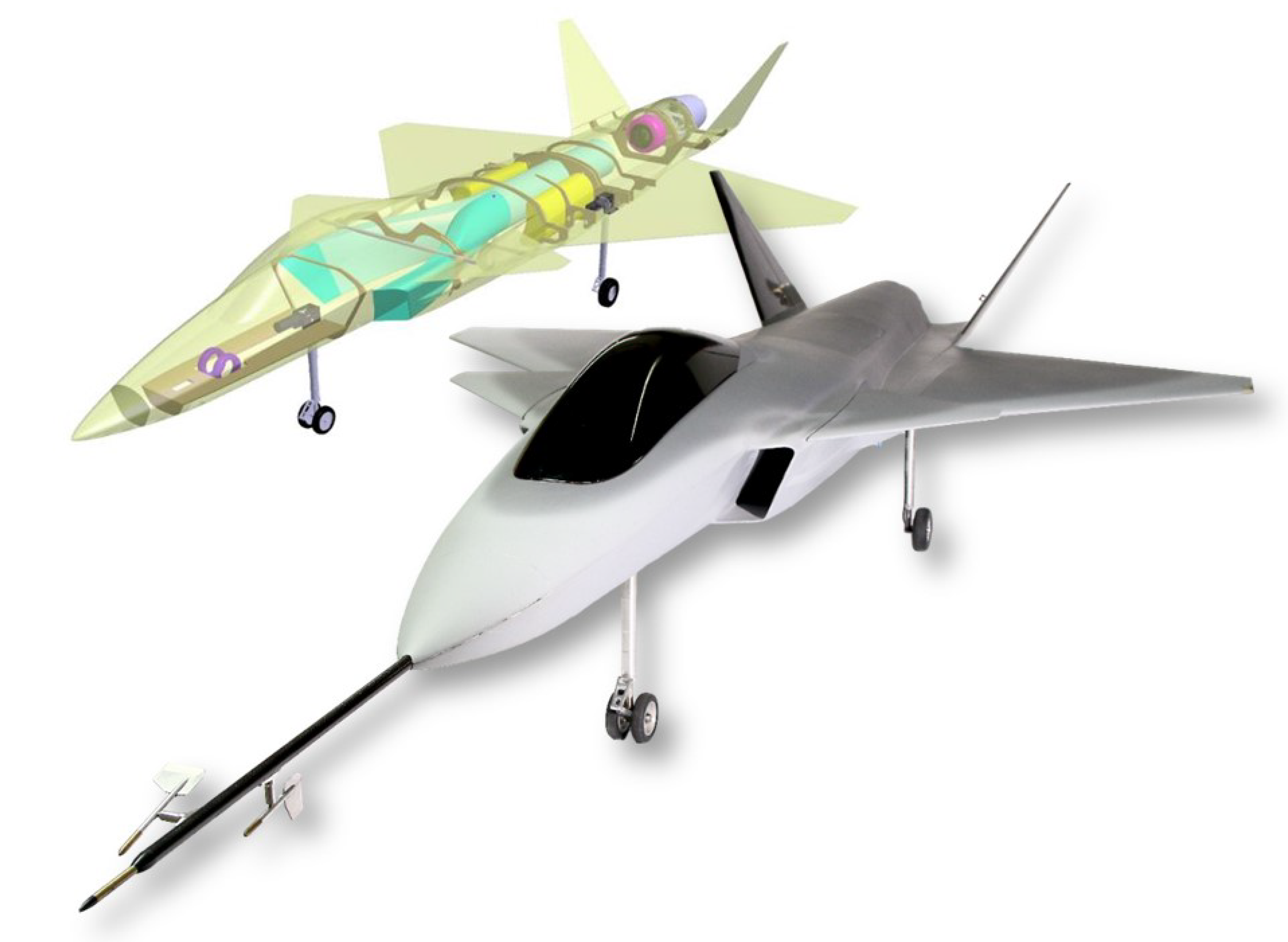
Due to its size and its instrumentation, the GFF subscale demonstrator was deemed a suitable platform to evaluate the usefulness of these methods. The GFF was a research study carried out during the NFFP4 Swedish National Aeronautical Research Program, and although it originated from a conceptual study at Saab, it is a generic design with no couplings to any Saab products. The GFF subscale demonstrator, shown in Figure 10, was originally built by Linköping University during that project and made its first flight in 2009 [15]. It is a radio-controlled jet-powered fighter with a close-coupled delta-wing canard configuration that reproduces the geometry of the full-scale GFF design at a $14\%$ scale. Dynamical scaling, using the Froude number as the similarity parameter [1,2], is achieved by adding extra weights at specific locations. However, the demonstrator is currently flown without extra ballast at a lower take-off weight in order to simplify its certification and operation in experiments that do not require extrapolation of results to the full-scale aircraft. Such was the case here, where the experiment was aimed at evaluating the method rather than to scale-up the obtained coefficients. The main characteristics of the subscale demonstrator at the moment of testing are given in

Table 2. Characteristics of the GFF subscale demonstrator during this experiment.

Scale	$14\%$
Length	$2.4$ m
Wing span	$1.5$ m
Typical take-off mass	19 kg
Typical fuel mass	3 kg
Engine	Jetcat P160
Maximum static thrust	160 N
Static margin	$+10\%$

.

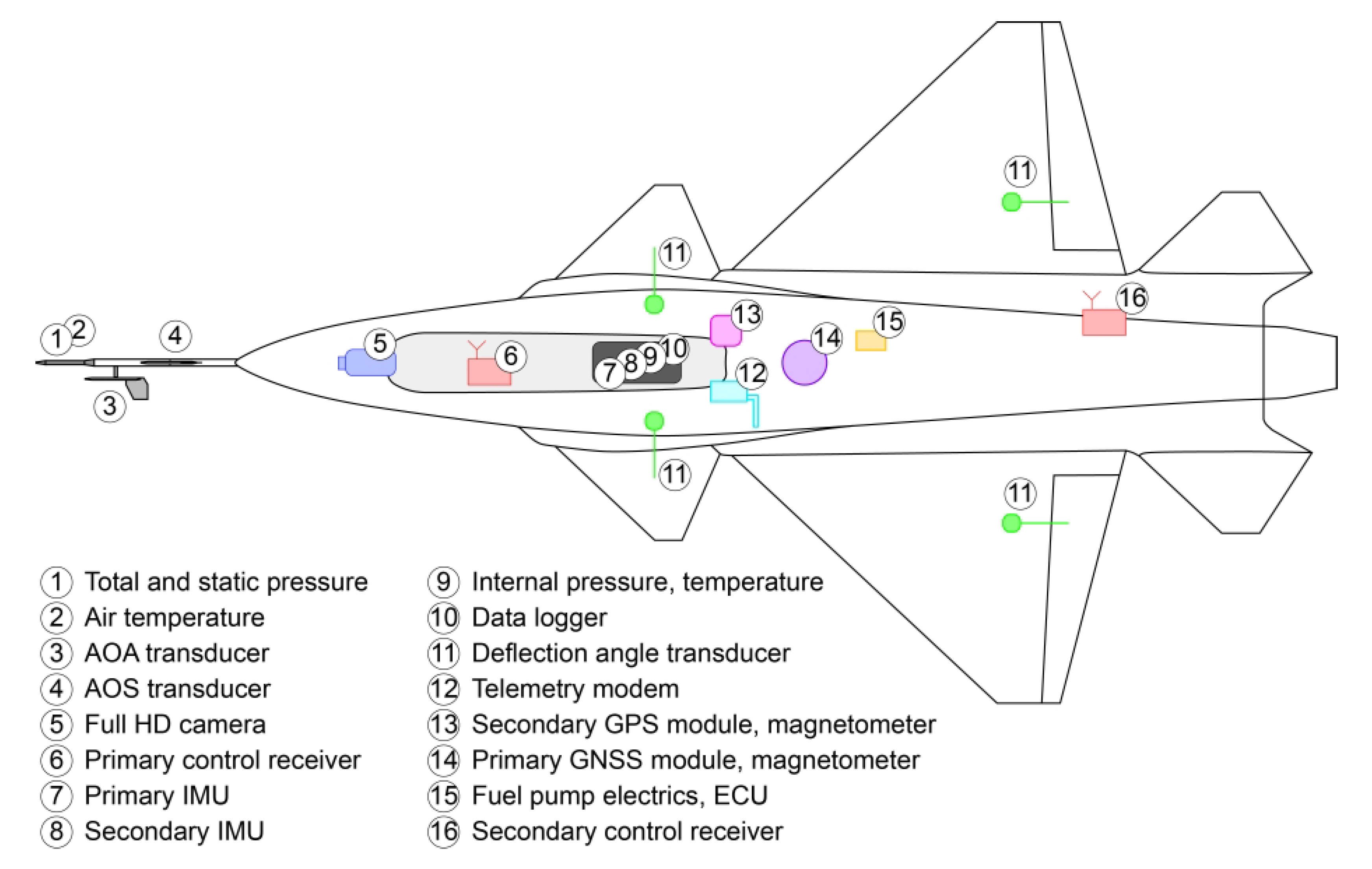
The GFF demonstrator is one of the platforms used in the MSDEMO and MESTA research programs for investigating the potential of subscale flight testing within aircraft conceptual design [9]. It is equipped with a data acquisition system and several sensors: Two inertial measurement units (IMU) provide accelerations and angular velocities. The IMUs together with redundant GPS receivers, magnetometers and air-pressure transducers are used to estimate the position, orientation and altitude. A custom-made nose-boom provides the airspeed, angle-of-attack and angle-of-sideslip using a pitot tube and contactless flow-angle transducers. The system also registers the incoming pilot commands and measures the real deflection of each control surface. These signals are logged on-board at an average sampling frequency of 100 Hz and also sent to a ground station in real time via a separate telemetry link. Figure 11 shows the layout of the data acquisition system.

While the GFF design represents a modern fighter aircraft with an augmented flight control system, the GFF subscale demonstrator was flown with open-loop control in a stable configuration to reduce risk and simplify its certification. After all, the methods studied here are appropriate for both stable and unstable systems and no significant information was omitted using this simplification. Furthermore, this experiment was limited to the evaluation of linear characteristics expected during the initial expansion of the flight envelope. The study of non-linear characteristics, typically found in these fighter configurations at the edges of the flight envelope, is usually a tedious and very specialized task that falls beyond the scope of this experiment.

Flight Test Procedure

The flight test campaign was carried out at a closed airfield located inside the controlled airspace of a nearby airport. Hence, all operations were carried out within VLOS and in contact with the corresponding air traffic control service. This type of operation severely constrains the available flight area, as shown in Figure 2; however, its main advantage is that it does not require a segregated airspace, a large infrastructure or a large team. Figure 12 describes the test procedure including the three main roles: one test conductor, responsible for controlling the test execution; one pilot, flying the aircraft from the ground control; and one test monitor, evaluating the test results between the flights and supervising the safety area. Test cards were used to predefine the manoeuvres to be performed in each flight. The corresponding commands and excitation signals were pre-programmed in advance and automatically executed from the radio-control transmitter by means of a novel flight test software program developed at Linköping University and described in [9]. This program augments the pilot control without requiring a closed-loop flight control system on-board. On the field, the easy adjustment and reconfiguration of the test sequences between flights also contributed to the agility and efficiency of this campaign.

The flight test was done during the evening to minimize the exposure to air turbulence; see Figure 13. Three flights of approximately 10 min of duration were completed. The first flight was dedicated to system checks and instrument calibration. The other two flights were dedicated to collect identification data. The first two of the nine multisine input signals, mentioned earlier in Section 3, were used both for parallel and separate excitation of the elevator and canard. The test program can be seen in

Table 3. Test program for identification.

Flight FT. $\#2$	Flight FT. $\#3$
Take-off and system checks	Take-off and system checks
Multisine 1 separated, MSs1	Multisine 1 parallel, MSp1
Multisine 1 separated, MSs1	Multisine 1 parallel, MSp1
Multisine 2 separated, MSs2	Multisine 2 parallel, MSp2
Multisine 1 parallel, MSp1	Multisine 1 separated, MSs1
Multisine 1 parallel, MSp1	Multisine 1 separated, MSs1
Multisine 2 parallel, MSp2	Multisine 2 separated, MSs2
Double pulse parallel, DPp	Double pulse separated, DPs
Approach and landing	Approach and landing

. The test setup was used to get repetitions of excitation for different fuel weights. The fuel weight is about $16\%$ of the take-off weight, and it can, therefore, have an effect on the results.

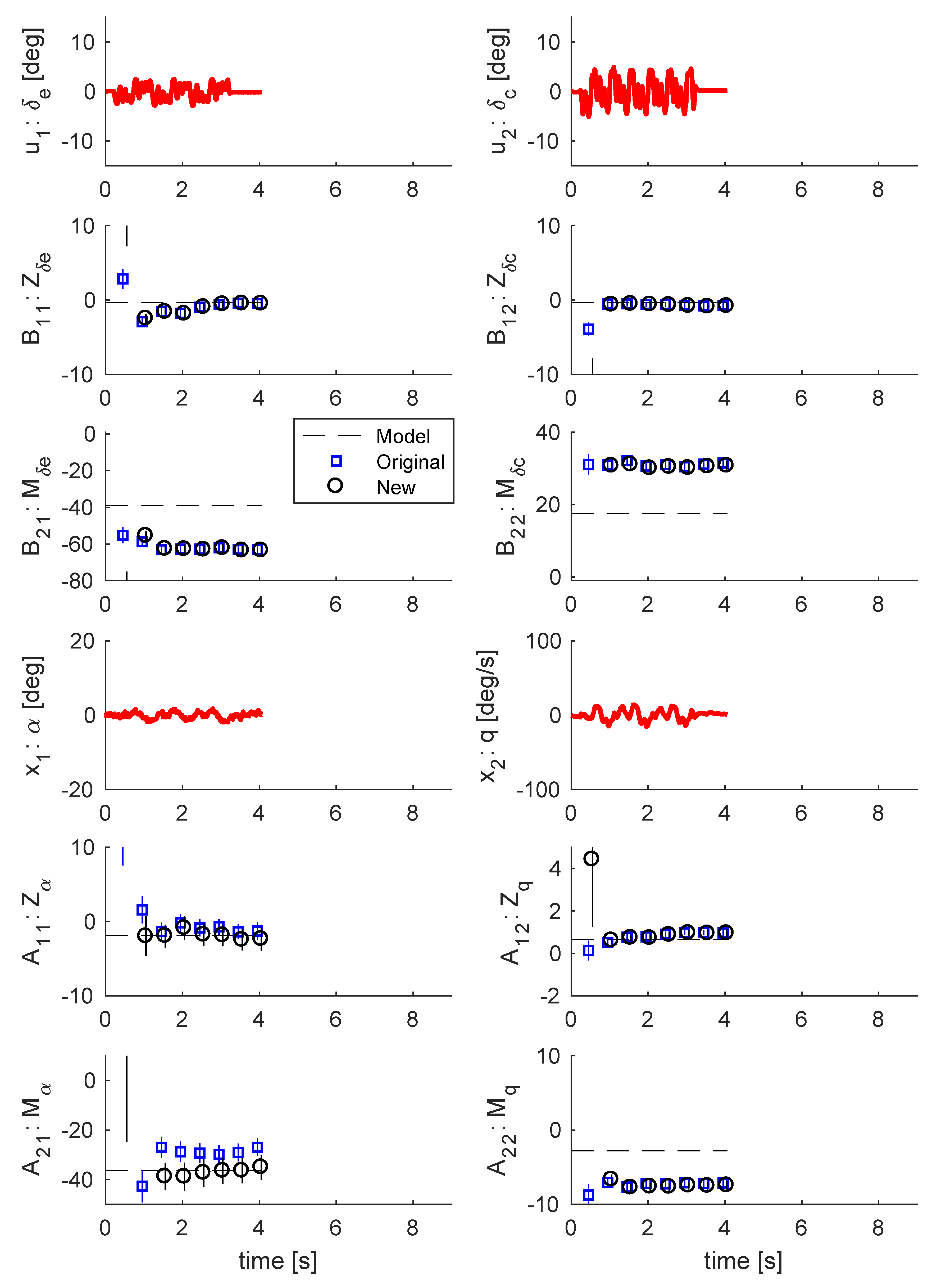
5. Results

Some examples of estimation results from the four different types of manoeuvres (multisine 1 separated (MSs), multisine parallel (MSp), double pulse parallel (DPp), double pulse separated (DPs)) defined in Table 3 are shown in Figure 14, Figure 15, Figure 16 and Figure 17. The test with the separated double pulse (DPs) had to be repeated twice during flight FT. $\#3$ since the first one was aborted due to ground proximity. This gave two realisations, DPs1 (aborted) and DPs2 (repeated). The repeated double pulse was used for the estimations. The figures show the flight test data in red and the model (17), based on earlier data, in a black dashed line. The estimated parameters are given as blue squares for the original method and as black circles for the new method. The estimated uncertainty measures of two standard deviations are shown as vertical bars. It should be noted that the model (17) is not the true system, but rather a reference that can be used to say if the flight test results show control effectiveness or stability characteristics that are different from the model. If these differences were large, they could motivate the decision to abort the test until the causes are investigated and understood.

When comparing the results in Figure 14 and Figure 15, the methods give quite similar estimates in the end for the separated and parallel multisine inputs. This can be seen in

Table 4. Comparison of the estimates for the crest factor optimized multisine (MS) input signal run separately and in parallel. The model (17) is given as a reference.

		Original		New
	Model	MSs1	MSp1	MSs1	MSp1
$Z_{\alpha }$	$-1.880$	$-1.322$	$-1.296$	$-3.939$	$-2.376$
$Z_q$	$0.651$	$0.926$	$0.962$	$1.205$	$0.945$
$Z_{{\delta }_e}$	$-0.332$	$1.288$	$-0.468$	$2.131$	$-0.499$
$Z_{{\delta }_c}$	$-0.367$	$-1.643$	$-0.703$	$-2.161$	$-0.821$
$M_{\alpha }$	$-36.395$	$-26.387$	$-26.959$	$-27.502$	$-35.076$
$M_q$	$-2.772$	$-7.078$	$-7.131$	$-8.080$	$-7.449$
$M_{{\delta }_e}$	$-39.044$	$-62.373$	$-62.951$	$-65.082$	$-63.570$
$M_{{\delta }_c}$	$17.488$	$34.231$	$31.444$	$35.329$	$30.688$

. The difference is during the test manoeuvres where the estimated canard effectivenesses $Z_{{\delta }_c}$ and $M_{{\delta }_c}$ are quite uncertain before the excitation for the separated manoeuvres, as should be expected.

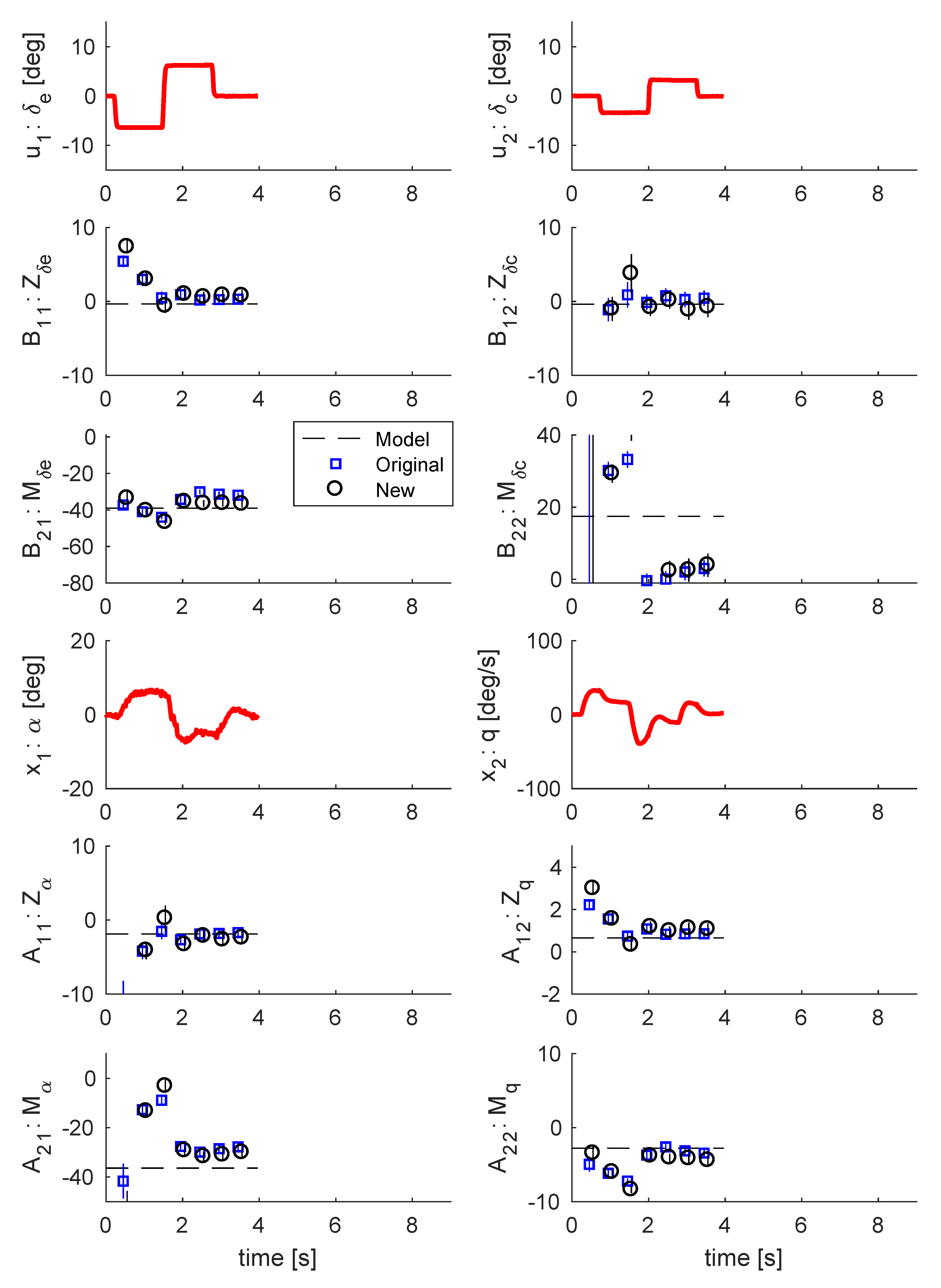
The differences are bigger when comparing the parallel multisine and double pulse in Figure 15 and Figure 16, predominantly in the pitching moment. The biggest difference is in the canard effectiveness $M_{{\delta }_c}$ where the estimated effectiveness is much lower for the double pulse input. A similar result can be seen when comparing the two double pulse inputs in Figure 16 and Figure 17. This can also be seen in

Table 5. Comparison of the estimates for the classic double pulse (DP) input signal run separately and in parallel. The model (17) is given as a reference.

		Original		New
	Model	DPp	DPs2	DPp	DPs2
$Z_{\alpha }$	$-1.880$	$-1.684$	$-1.938$	$-2.397$	$-2.600$
$Z_q$	$0.651$	$0.851$	$0.645$	$1.072$	$1.000$
$Z_{{\delta }_e}$	$-0.332$	$0.306$	$0.078$	$0.767$	$1.061$
$Z_{{\delta }_c}$	$-0.367$	$0.450$	$-0.613$	$-0.730$	$-1.306$
$M_{\alpha }$	$-36.395$	$-27.740$	$-26.251$	$-30.032$	$-28.269$
$M_q$	$-2.772$	$-3.431$	$-4.664$	$-4.408$	$-8.804$
$M_{{\delta }_e}$	$-39.044$	$-31.932$	$-40.702$	$-36.745$	$-58.807$
$M_{{\delta }_c}$	$17.488$	$3.048$	$22.343$	$3.933$	$33.533$

.

The results from the repeated separated double pulse (DPs2) are shown in Figure 17. It gives not exact, but similar results to the separated multisine in Figure 14 when using the new method. It can also be seen that the difference between the estimates of the original method and the new method are largest for this manoeuvre.

In

Table 6. Absolute value of the correlation between the real part of the regressors.

	MSs1				MSp1
	${\mathbf{\delta }}_{\mathit{e}}$	${\mathbf{\delta }}_{\mathit{c}}$	$\mathbf{\alpha }$	$\mathit{q}$	${\mathbf{\delta }}_{\mathit{e}}$	${\mathbf{\delta }}_{\mathit{c}}$	$\mathbf{\alpha }$	$\mathit{q}$
${\delta }_e$	$1.00$	$0.07$	$0.04$	$0.18$	$1.00$	$0.08$	$0.02$	$0.35$
${\delta }_c$		$1.00$	$0.42$	$0.34$		$1.00$	$0.40$	$0.22$
$\alpha$			$1.00$	$0.06$			$1.00$	$0.06$
q				$1.00$				$1.00$
	DPp				DPs2
	${\mathbf{\delta }}_{\mathit{e}}$	${\mathbf{\delta }}_{\mathit{c}}$	$\mathbf{\alpha }$	$\mathit{q}$	${\mathbf{\delta }}_{\mathit{e}}$	${\mathbf{\delta }}_{\mathit{c}}$	$\mathbf{\alpha }$	$\mathit{q}$
${\delta }_e$	$1.00$	$0.61$	$0.78$	$0.72$	$1.00$	$0.68$	$0.54$	$0.49$
${\delta }_c$		$1.00$	$0.86$	$0.03$		$1.00$	$0.58$	$0.70$
$\alpha$			$1.00$	$0.42$			$1.00$	$0.04$
q				$1.00$				$1.00$

, the absolute values of correlation between the real part of the regressors are given. The multisine input signals have a much lower correlation than the double pulses. The parallel double pulse, DPp, has the highest correlation of $0.86$. This might reduce the resulting estimation accuracy.

The validation of the estimated models is an important part of system identification [17,20]. The flight manoeuvre FT. $\#3$, DPs1, which was aborted due to a ground proximity warning, was used as the test dataset to validate the different estimated models. A common measure for judging how well a model, m, can explain the information in the validation dataset, Z, is the model fit criterion defined as:

$$F(m,Z)=100(1-\frac{\parallel y-\widehat{y}{(\theta )\parallel }_2}{\parallel y-\overline{y}{\parallel }_2})$$

(20)

where ${\parallel }_2$ indicates the two-norm of a vector.

This was used to compare the original and new method. The results are shown in

Table 7. Comparison of the original and new method using the aborted test manoeuvre DPs1 as validation data and the model fit criterion as a measure.

Flight FT. $\#2$			Flight FT. $\#3$
Manoeuvre	Original	New	Manoeuvre	Original	New
MSs1	$62.5\%$	$66.7\%$	MSp1	$50.3\%$	$47.0\%$
MSs1	$50.2\%$	$63.0\%$	MSp1	$50.5\%$	$47.6\%$
MSs2	$-12.4\%$	$39.8\%$	MSp2	$68.3\%$	$68.9\%$
MSp1	$54.5\%$	$60.8\%$	MSs1	$62.5\%$	$68.1\%$
MSp1	$57.5\%$	$67.7\%$	MSs1	$54.9\%$	$62.0\%$
MSp2	$66.3\%$	$67.7\%$	MSs2	$55.2\%$	$64.3\%$
DPp	$26.1\%$	$41.9\%$	DPs2	$69.9\%$	$70.5\%$

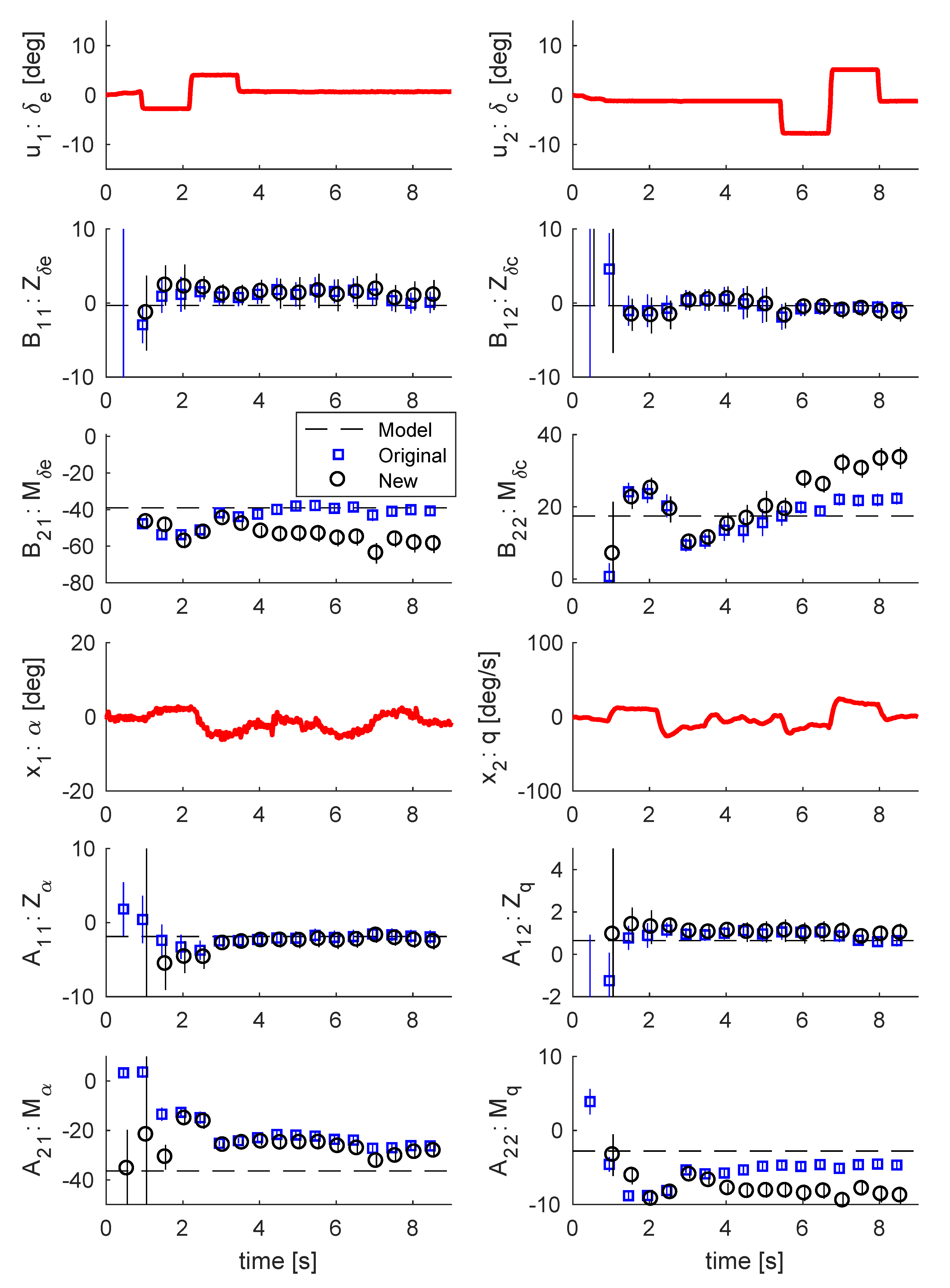
and Figure 18. Two things can be noted. First, the new method gives in general a better model fit than the original method. This means that the addition of instrumental variables contributes in a positive way. Second, the double pulse excitation gives a lower model fit than the multisine input with one exception. This may indicate that it is beneficial to use multisine inputs for this type of subscale flight testing.

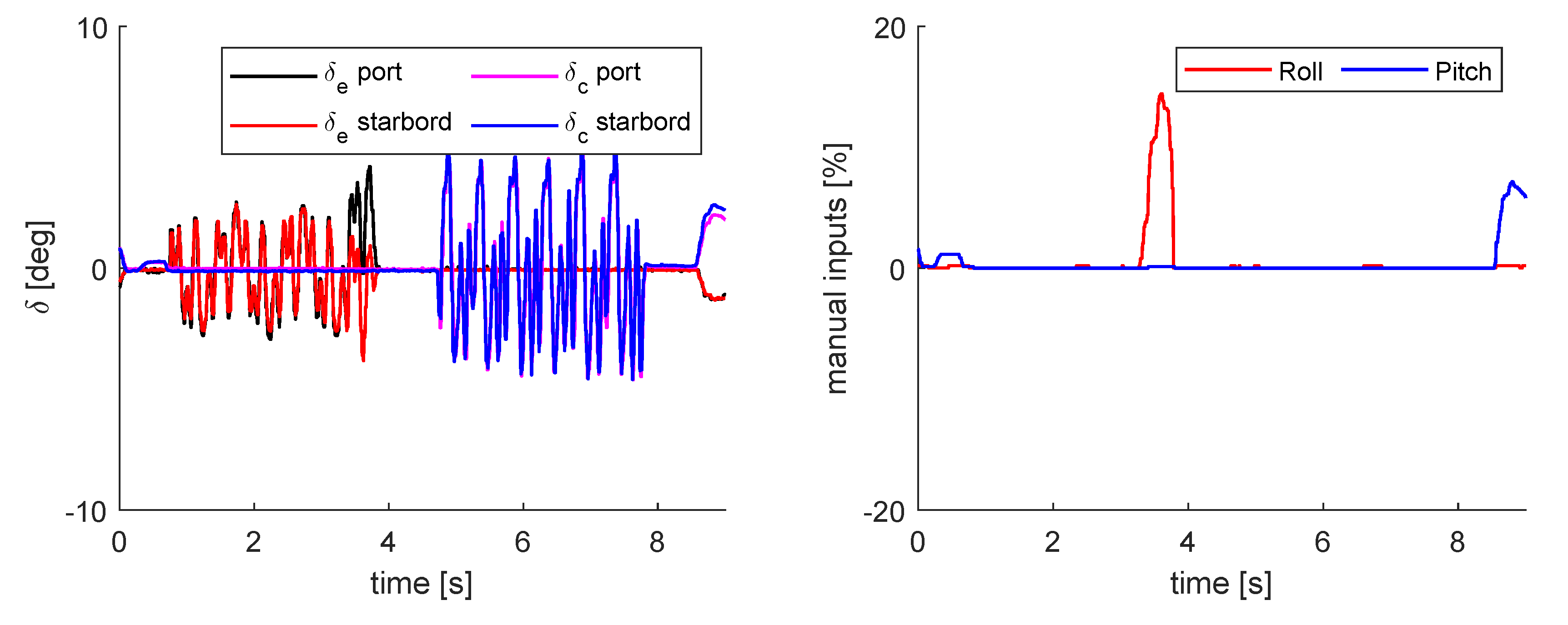
The results shown in Table 7 show an unexpected poor fit for manoeuvre MSs2 in Flight FT. $\#2$. The flight test data reveal that the pilot commanded a sudden roll correction during the execution of this manoeuvre, as shown in Figure 19. The disturbance caused by this correction may explain the poor fit associated with this manoeuvre.

6. Post Flight Analysis

In post flight analysis, all test manoeuvres are available and can be used together. Doing this will improve the estimation result since the information content available is much larger than for each individual manoeuvre. The aborted manoeuvre, DPs1 in Flight FT. $\#3$, again was used as the test data for validation while all 14 remaining manoeuvres given in Table 3, including DPs2 in Flight FT. $\#3$, were used for model construction.

A data fusion approach, like the one given in [21], can be used to combine models from different manoeuvres into one single model. The model fusion is a weighted average of estimates ${\widehat{\theta }}_k,k=1\dots K$, where the weights are the information matrices ${\widehat{I}}_k={\widehat{P}}_k^{-1}$ from different time sequences. The model fusion is therefore given as:

$$\begin{array}{cc}\hfill \widehat{I}& =\sum _{k=1}^K{\widehat{I}}_k\hfill \\ \hfill \widehat{\theta }& ={\widehat{I}}^{-1}\sum _{k=1}^K{\widehat{I}}_k{\widehat{\theta }}_k\hfill \end{array}$$

(21)

For the original method, the resulting model becomes:

$$\begin{array}{cc}\hfill \dot{x}(t)& =\left[\begin{array}{cc}-1.90& 1.03\\ -24.52& -7.11\end{array}\right]x(t)+\left[\begin{array}{cc}0.90& -1.27\\ -51.25& 29.43\end{array}\right]u(t)\hfill \\ \hfill y(t)& =\left[\begin{array}{cc}1.00& 0.00\\ 0.00& 1.00\end{array}\right]x(t)\hfill \end{array}$$

(22)

while for the new method, the resulting model becomes:

$$\begin{array}{cc}\hfill \dot{x}(t)& =\left[\begin{array}{cc}-2.74& 1.14\\ -26.29& -8.30\end{array}\right]x(t)+\left[\begin{array}{cc}0.90& -1.46\\ -55.61& 30.70\end{array}\right]u(t)\hfill \\ \hfill y(t)& =\left[\begin{array}{cc}1.00& 0.00\\ 0.00& 1.00\end{array}\right]x(t)\hfill \end{array}$$

(23)

The validation of these models using the DPs1 dataset produces the results shown in Figure 20, where the initial model (17) is also included for reference. The resulting models for both the original and the new method are similar, and they give a satisfactory fit of $68.4\%$ and $67.9\%$, respectively. The initial, pre-flight model (17) presents a less damped behaviour and gives a poorer fit of $54.0\%$. The similarity of the results for the original and the new method could be motivated by an averaging effect, since the estimates are based on the entire dataset.

7. Conclusions

This paper describes a method to improve the flight testing of remotely piloted aircraft for system identification of linear flight mechanical characteristics, especially when flying near the ground within a limited distance. The focus is on increasing the efficiency of flight envelope expansion tests by using real-time identification and dealing with two major issues: the short time available for each manoeuvre and the large exposure to air turbulence.

The authors make use of a relatively simple software solution to command tailored multisine input signals from a conventional radio transmitter without the need for complex on-board systems. These signals, designed according to the basic data available from previous flights, present a low correlation between the different inputs and could be applied simultaneously to different control surfaces. Results from a flight test with a subscale jet aircraft support the idea that the estimated parameters from the simultaneous multisine inputs are similar to those obtained with sequential ones, while the excitation time could be reduced by almost 50%. In addition, both multisine approaches seem to give better results than more traditional pulse inputs.

Two different methods are used for the analysis of flight test data: The first uses an existing real-time frequency domain approach, denoted here as the original method. The second incorporates instrumental variables in the original method. Results from the subscale flight test suggest that this new method improves the accuracy of the estimations for data affected by turbulent conditions.

All methods, procedures and results described in this paper contribute to reducing the gap between relatively simple and cost-effective subscale flight tests and more ambitious, resource-intensive flight test campaigns. This supports both the development of UASs, as well as the use of SFT as an economical tool for risk reduction during the early stages of full-scale aircraft design.

References

1. Wolowicz, C.H.; Bowman, J.S.; Gilbert, W.P. Similitude Requirements and Scaling Relationships as Applied to Model Testing; Technical Paper 1435; NASA: Washington, DC, USA, 1979. [Google Scholar]
2. Chambers, J.R. Modeling Flight: The Role of Dynamically Scaled Free-Flight Models in Support of NASA’s Aerospace Programs, 1st ed.; NASA: Washington, DC, USA, 2009; p. 202. [Google Scholar]
3. Walker, L.A. Flight Testing the X-36—The Test Pilot’s Perspective; Contractor Report 198058; NASA: Washington, DC, USA, 1997. [Google Scholar]
4. Risch, T.; Cosentino, G.; Regan, C.; Kisska, M.; Princen, N. X-48B Flight Test Progress Overview. In Proceedings of the 47th AIAA Aerospace Sciences Meeting including The New Horizons Forum and Aerospace Exposition, Orlando, FL, USA, 5–8 January 2009; AIAA: Reston, VA, USA, 2009. [Google Scholar]
5. Bushnell, D.M. Scaling: Wind Tunnel to Flight. Annu. Rev. Fluid Mech. 2006, 38, 111–128. [Google Scholar] [CrossRef]
6. Jordan, T.; Langford, W.; Hill, J. Airborne Subscale Transport Aircraft Research Testbed—Aircraft Model Development. In Proceedings of the AIAA Guidance Navigation, and Control Conference and Exhibit, San Francisco, CA, USA, 15–18 August 2005; AIAA: San Fracisco, CA, USA, 2005. [Google Scholar]
7. Jouannet, C.; Lundström, D.; Amadori, K.; Berry, P. Design of a Very Light Jet and a Dynamically Scaled Demonstrator. In Proceedings of the 46th AIAA Aerospace Sciences Meeting and Exhibit, Reno, NV, USA, 7–10 January 2008. [Google Scholar]
8. Bailey, R.M.; Hostetler, R.W.; Barnes, K.N.; Belcastro, C.M.; Belcastro, C.M. Experimental Validation: Subscale Aircraft Ground Facilities and Integrated Test Capability. In Proceedings of the American Institute of Aeronautics and Astronautics Guidance, Navigation and Control Conference, Chicago, IL, USA, 10–13 August 2009; AIAA: San Fracisco, CA, USA, 2005. [Google Scholar]
9. Sobron, A. On Subscale Flight Testing: Applications in Aircraft Conceptual Design. Licentiate Thesis, Linköping University, Linköping, Sweden, 2018. [Google Scholar] [CrossRef]
10. Stahl, P.; Sendner, F.M.; Rößler, C.; Hornung, M.; Hermanutz, A. Mission and Aircraft Design of FLEXOP Unmanned Flying Demonstrator to Test Flutter Suppression within Visual Line of Sight. In Proceedings of the 17th AIAA Aviation Technology Integration, and Operations Conference, Denver, CO, USA, 5–9 June 2017; AIAA: Denver, CO, USA, 2017. [Google Scholar] [CrossRef]
11. Morelli, E.A. Flight Test Maneuvers for Efficient Aerodynamic Modeling. J. Aircr. 2012, 49, 1857–1867. [Google Scholar] [CrossRef] [Green Version]
12. Jategaonkar, R.V.; Plaetschke, E. Algorithms for aircraft parameter estimation accounting for process and measurement noise. J. Aircr. 1989, 26, 360–372. [Google Scholar] [CrossRef]
13. Larsson, R.; Enqvist, M. Sequential Aerodynamic Model Parameter Identification. IFAC Proc. Vol. 2012, 45, 1413–1418. [Google Scholar] [CrossRef]
14. Morelli, E.A.; Klein, V. Aircraft System Identification: Theory and Practice, 2nd ed.; Sunflyte Enterprises: Williamburg, VA, USA, 2016. [Google Scholar]
15. Jouannet, C.; Berry, P.; Melin, T.; Amadori, K.; Lundström, D.; Staack, I. Subscale flight testing used in conceptual design. Aircr. Eng. Aerosp. Technol. 2012, 84, 192–199. [Google Scholar] [CrossRef]
16. Lundström, D.; Sobron, A.; Krus, P.; Jouannet, C.; da Silva, R.G.A. Subscale Flight Testing of a Generic Fighter Aircraft. In Proceedings of the 30th Congress of the International Council of the Aeronautical Sciences, Daejeon, Korea, 25–30 September 2016. [Google Scholar]
17. Ljung, L. System Identification: Theory for the User, 2nd ed.; Prentice Hall PTR: Upper Saddle River, NJ, USA, 1999. [Google Scholar]
18. Kollár, I.; Pintelon, R.; Schoukens, J. Frequency domain system identification toolbox for matlab: Characterizing nonlinear errors of linear models. IFAC Proc. Vol. 2006, 39, 726–731. [Google Scholar] [CrossRef] [Green Version]
19. Schoukens, J.; Vaes, M.; Pintelon, R. Linear system identification in a nonlinear setting: Nonparametric analysis of the nonlinear distortions and their impact on the best linear approximation. IEEE Control Syst. 2016, 36, 38–69. [Google Scholar]
20. Morelli, E.A.; Klein, V. Application of system identification to aircraft at NASA langley research center. J. Aircr. 2005, 42, 12–25. [Google Scholar] [CrossRef]
21. Gustafsson, F. Statistical Sensor Fusion; Studentliteratur: Lund, Sweden, 2012. [Google Scholar]
Figure 1. An early example of subscale flight testing to assess low-speed control characteristics of an unconventional configuration: initial development of the Saab 35 Draken, ca. 1949. Courtesy of Saab.
Aerospace 07 00135 g001
Figure 2. A typical flight within VLOS is a challenging environment for excitation and identification. The short time available and the ground turbulence require special consideration.
Aerospace 07 00135 g002
Figure 3. Definition of the model variables. Note that Z in (16) is the same as N in the figure.
Aerospace 07 00135 g003
Figure 4. Estimation data from earlier flight tests. Test data are shown in red, while simulated model data are shown in black for the states angle-of-attack and pitch rate.
Aerospace 07 00135 g004
Figure 5. Validation data from earlier flight tests. Test data are shown in red, while simulated model data are shown in black for the states angle-of-attack and pitch rate.
Aerospace 07 00135 g005
Figure 6. A double pulse (DP) input (left) and a crest factor optimized multisine (MS) input (right).
Aerospace 07 00135 g006
Figure 7. Amplitudes (left) and phases (right) of the multisine frequency separated elevator and canard input signals. The phases corresponding to low-amplitude frequencies are omitted in the right figure. The excitation has odd frequencies for the elevator (red) and even for the canard (black).
Aerospace 07 00135 g007
Figure 8. Bode plot of the Generic Future Fighter (GFF) demonstrator (red) and the Gripen (black).
Aerospace 07 00135 g008
Figure 9. Simulations with different input signals. Crest factor optimized multisine (red) vs. double pulse (black).
Aerospace 07 00135 g009
Figure 10. Overview of the GFF subscale demonstrator.
Aerospace 07 00135 g010
Figure 11. Layout of the data acquisition system on the GFF platform.
Aerospace 07 00135 g011
Figure 12. Procedure for flight testing within VLOS. The input signals are injected from the control transmitter using a specially-developed software.
Aerospace 07 00135 g012
Figure 13. GFF demonstrator on final approach with gear down as seen from external and on-board cameras.
Aerospace 07 00135 g013
Figure 14. Results from flight FT. # 2 with manoeuvre MSs1. The flight test data are shown in red, the results from the original method as blue squares and the results from the new method as black circles. The uncertainties are given as vertical bars. Note that the model (17) is not the true system.
Aerospace 07 00135 g014
Figure 15. Results from flight FT. # 2 with manoeuvre MSp1. The flight test data are shown in red, the results from the original method as blue squares and the results from the new method as black circles. The uncertainties are given as vertical bars. Note that the model (17) is not the true system.
Aerospace 07 00135 g015
Figure 16. Results from flight FT. # 2 with manoeuvre DPp. The flight test data are shown in red, the results from the original method as blue squares and the results from the new method as black circles. The uncertainties are given as vertical bars. Note that the model (17) is not the true system.
Aerospace 07 00135 g016
Figure 17. Results from flight FT. # 3 with manoeuvre DPs2. The flight test data is shown in red, the results from the original method as blue squares and the results from the new method as black circles. The uncertainties are given as vertical bars. Note that the model (17) is not the true system.
Aerospace 07 00135 g017
Figure 18. Validation simulations with flight test data in red. Upper: input, middle: output original method and bottom: output new method.
Aerospace 07 00135 g018
Figure 19. Flight test data showing a sudden roll correction commanded by the pilot during manoeuvre MSs2 in Flight FT. # 2 . This disturbance may explain the poor fit obtained for this manoeuvre.
Aerospace 07 00135 g019
Figure 20. Validation simulations with flight test data in red.
Aerospace 07 00135 g020