Article

Sequential Low-Thrust Orbit-Raising of All-Electric Satellites

Aerospace Engineering , Wichita State University, 1845 Fairmount St Box 42, Wichita, KS 67260, USA
*
Author to whom correspondence should be addressed.
Aerospace 2020, 7(6), 74; https://doi.org/10.3390/aerospace7060074
Submission received: 6 March 2020 / Revised: 17 May 2020 / Accepted: 26 May 2020 / Published: 4 June 2020
(This article belongs to the Special Issue Electric Propulsion)

Abstract

:
In this paper, we consider a recently developed formulation of the electric orbit-raising problem that utilizes a novel dynamic model and a sequence of optimal control sub-problems to yield fast and robust computations of low-thrust trajectories. This paper proposes two enhancements of the computational framework. First, we use thruster efficiency in order to determine the trajectory segments over which the spacecraft coasts. Second, we propose the use of a neural network to compute the solar array degradation in the Van Allen radiation belts. The neural network is trained on AP-9 data and SPENVIS in order to compute the associated power loss. The proposed methodology is demonstrated by considering transfers from different geosynchronous transfer orbits. Numerical simulations analyzing the effect of thruster efficiency and average power degradation indicate the suitability of starting the maneuver from super-geosynchronous transfer orbits in order to limit fuel expenditure and radiation damage. Furthermore, numerical simulations demonstrate that proposed enhancements are achieved with only marginal increase in computational runtime, thereby still facilitating rapid exploration of all-electric mission scenarios.

1. Introduction

In recent years, enhancements to solar-electric propulsion technology [1,2,3] have seen their greater usage in Earth-orbiting satellites [1,4,5], for both station-keeping as well as orbital transfer purposes [5]. These applications have largely been for relatively larger satellites, and a variety of electric propulsion technologies are currently being miniaturized for future incorporation in nano-satellites as well [6,7]. The primary focus of this paper is the electric orbit-raising maneuver during the deployment of satellites operating in the geosynchronous equatorial orbit (GEO). The telecommunication satellite industry has started adopting electric propulsion for performing long-time scale orbit-raising maneuvers to the GEO. Instances include the deployment of SatMex and ABS satellites using Boeing’s 702-SP all-electric architecture (2015) [8], and that of the EutelSat 172B satellite using Airbus’ fully-electric propulsion system (2017) [9], as well as China’s SJ-13 mission (2017) [10]. As more future space missions begin incorporating electric orbit-raising to GEO, there is a need for efficient mission design tools to address the challenges associated with the complicated maneuver spanning several months. In particular, we are interested in tools that facilitate fast and robust analysis of numerous electric orbit-raising scenarios to help identify best technology selections for the satellite bus.
The main challenge of the long-duration electric orbit-raising maneuver arises due to the low acceleration imparted by the onboard electric propulsion systems, relative to the local gravitational acceleration due to the Earth. The multiple eclipses that the satellite encounters en route to GEO deprive the electric propulsion system of power from the solar arrays, thereby adding to the complexity of the transfer.
For instance, Figure 1 depicts a 225-revolution low-thrust transfer trajectory from a geosynchronous transfer orbit (GTO) to the GEO, spanning more than five months. Such a multi-revolution long duration transfer means a long transit time through the Van Allen belts, causing damage to the solar arrays, and therefore impacting thrust availability during the transfer. Mission design for an all-electric satellite therefore involves identifying various variables that affect the orbit-raising maneuver: number and type of electric thrusters for the satellite’s propulsion system, sizing of the solar array and shielding requirements, battery sizing in case thrusters need to be supported during eclipses, launch vehicle and injection orbit elements. In this paper, we consider a computational framework to generate low-thrust orbit-raising trajectories in a fast, robust, and automated manner, in order to facilitate automated analysis of numerous orbit-raising trajectories as part of exploring the design space.
The computation of an all-electric orbit-raising trajectory requires the solution of a challenging optimal control problem. A number of methods have been developed in order to compute optimal low-thrust orbit-raising trajectory, broadly falling under the categories of direct and indirect optimization based methodologies. While indirect techniques use calculus of variations to determine the necessary conditions of optimality and set up a two-point boundary value problem [11,12,13,14,15,16], direct techniques avoid using calculus of variations and instead rely on direct transcription and collocation to set up a parameter optimization problem, often solved using commercial software such as SNOPT and IPOPT [17,18,19,20,21]. These methodologies typically rely on good quality user-provided initial guesses in order to rely on numerical convergence of the underlying algorithm [22]. In order to address these issues, a number of alternative approaches approaches have been developed, such as shape-based techniques, Q-law, or semi-analytical approaches [23,24,25,26,27,28,29,30,31,32,33,34,35,36,37]. Furthermore, dynamic models to capture the underlying translation dynamics of the spacecraft often play an important role in the convergence of direct or indirect optimization techniques, and several such models have been used in the literature, orbital elements, equinoctial elements, Cartesian, and spherical coordinates; please see Ref. [38] for a comparison of different dynamic models in terms of their impact on the numerical solutions of orbit-raising optimal control problems.
This paper utilizes a novel dynamic model that has proven to be effective for solving orbit-raising optimal control problems [38,39]. This model uses dynamical parameters as the states of the spacecraft, instead of geometrical quantities. This model also uses a non-inertial reference frame that can be obtained by a 2-1-3 rotation sequence of Euler angles instead of a traditional 3-1-3 rotation sequence used in the orbital mechanics. This dynamic model removes the singularity arising for both equatorial and circular orbits, the singularity being a major drawback with traditional orbital elements. The singularity is shifted to a special case of polar orbits when the right ascension of the ascending node is 0 or 2 π deg. Five out of this six new orbital elements are regularized, that is, they change very slowly for a thrusting spacecraft and remain constant for pure Keplerian motion. This makes them suitable for the trajectory optimization schemes that compute trajectories for long-time-scale transfers. Additionally, the current paper utilizes a novel optimization scheme introduced in Ref. [39]; this technique breaks the multi-revolution problem into a sequence of optimization sub-problems, computing the all-electric orbit-raising trajectory in the order of tens of seconds on a standard personal computer without the need of any user-provided initial guess. This optimization tool can be used to analyze various electric orbit-raising mission scenarios and also can compute the trajectories to the GEO due to the non-singularity of the formulation in the equatorial plane. Recently, the work in Ref. [39] was extended in order to analyze a variety of different aspects of the orbit-raising problem: effect of J 2 perturbations and accurate shadow model [40], effects of using different types of electric thrusters [41], analysis of attitude control during the maneuver [42], effect of planning horizon length [43], effect of objective function weights [44], and their adaptive modification [45].
The contributions of the paper are two important enhancements of the optimization problem described in Ref. [39], in which the thrust magnitude was determined by a pre-set scheme (thrust in Sun-lit segments of trajectory and coast in eclipses) and power loss during transfer was not considered. First, we allow for coasting arcs within the Sun-lit portion of the orbit-raising trajectory. This is achieved through the application of the concept of thruster efficiency originally proposed by Petropoulos [46] for the Q-law based framework. The thruster efficiency is defined for each segment of discretized trajectory in the optimization sub-problem, and allows for deciding the thrust magnitude. This enhancement is important to identify trade-offs between deployed mass and deployment time for the satellite. Second, we also allow for the consideration of radiation damage within the optimization framework, by proposing a neural network, trained on AP-9 radiation data that computes the radiation damage over a revolution based on the osculating orbital elements. The neural network predicts the power degradation over a revolution, and updates the thrust availability for the next revolution. Prior efforts on capturing the radiation dose were an analytical model based on AP-8 data [47] and semi-analytical approach utilizing AP-9 data and the SCREAM software [48]; however, to the best of knowledge of the authors, there has not been any effort on utilizing a neural network based modeling of the solar array degradation. The paper is organized as follows: we first present the mathematical overview of the problem under consideration, then elaborate the two proposed extensions, and finally present numerical simulations to demonstrate our proposed methodology.

2. Problem Formulation

In this section, we provide a formulation of the low-thrust orbit-raising problem modeled as a sequence of optimal control sub-problems.

2.1. Spacecraft Dynamics

In order to describe the dynamics of the spacecraft, we consider two reference frames: the standard geocentric equatorial inertial reference frame I , and an orbital reference frame O obtained after a 2-1 rotation sequence of the inertial reference frame. The dynamic model utilizes the following states of the spacecraft: magnitude of the specific angular momentum vector h, the components of specific angular momentum vector h X and h Y in the xy plane of I , the components e x and e y of the eccentricity vector in the xy plane of the reference frame O , and an angle ϕ that locates the spacecraft. Rotating the reference frame O by angle ϕ in the orbital plane aligns it with a non-inertial frame N with axes along the radial direction, the normal to the orbital plane and the in-plane transverse direction. The control variables are given by the thrust components F r in the radial direction, F n in the transverse direction (in-plane) and out-of-plane F h perpendicular to F r and F n . These components of the thrust are functions of the magnitude of thrust F and the control angles α and β as shown in Figure 2.
The first-order differential equations that describe the spacecraft translational dynamics are given by the following equations [39]:
h ˙ h X ˙ h Y ˙ e x ˙ e y ˙ ϕ ˙ = 0 0 0 0 0 μ 2 B 2 h 3 h h X h Y e x e y ϕ + G F r F n F h .
In the above-mentioned equations of motion for the spacecraft, the functions A and B are given by A = e x sin ϕ e y cos ϕ and B = 1 + e x cos ϕ + e y sin ϕ , while the matrix G maps the non-Keplerian acceleration terms to the rates of change of the state variables [39]:
G = 0 h 2 μ m B μ 2 B 2 h 3 0 h h x μ m B h 2 h 2 h X 2 h Y 2 μ m B h 2 h Y 2 sin ϕ + h h X h Y μ m B h 2 h Y 2 cos ϕ 0 h h y μ m B h h 2 h Y 2 μ m B cos ϕ h sin ϕ μ m 2 h cos ϕ μ m + h A sin ϕ μ m B h e y h Y μ m B h 2 h Y 2 sin ϕ h cos ϕ μ m 2 h sin ϕ μ m h A cos ϕ μ m B h e x h Y μ m B h 2 h Y 2 sin ϕ 0 0 h h Y μ m B h 2 h Y 2 sin ϕ
There is a unique transformation from the above-mentioned state variables and the commonly used variables used by the astrodynamics community, such as orbital elements or Cartesian states. For instance, if the position and velocity vectors of the spacecraft are known, then the angular momentum vector is obtained by their cross-product states, with h being the magnitude and h X , h Y being the components in the inertial reference frame. The eccentricity vector is also a function of the position and velocity vectors, and its components e x and e y are computed in the non-inertial frame O whose orientation with respect to the inertial frame is given by the following direction cosine matrix:
R = h Z h X 2 + h Z 2 0 h X h X 2 + h Z 2 h Y h X h h X 2 + h Z 2 h X 2 + h Z 2 h h Y h Z h h X 2 + h Z 2 h X h h Y h h Z h
The angle ϕ is then the angle between the position vector of the spacecraft and the x-axis of the reference frame O . For details, please refer to Ref. [39]. For convenience of the following discussion, we collectively represent the state variables h, h X , h Y , e x and e y using the vector x because these variables are “slow,” meaning that they vary slowly (in comparison to the sixth variable ϕ ) under the influence of low thrust, and are helpful for the convergence of numerical trajectory optimization solvers. During the transfer, the spacecraft passes through the shadow of Earth that affect its thrust capabilities. In the absence of solar power, the spacecraft cannot generate power, unless electric thrusters are powered by onboard energy storage. In the context of this paper, we consider that there is no thrust available during eclipses, meaning that, in the shadow of the Earth, the trajectory of the spacecraft is a conic section in the absence of orbital perturbations.

2.2. Sequential Orbit-Raising

In general, the low-thrust orbit-raising problem can be written as an optimal control problem to minimize the transfer time t f to raise the orbit of the spacecraft starting from initial state variables x0 to the final state variables xGE0, subject to the equations of motion for the spacecraft and other associated constraints (such as no thrusting in eclipses). As already explained, we instead formulate a sequence of optimal control sub-problems, with each sub-problem decides on the optimal thrust scheme over a revolution (defined by a change of ϕ by 2 π ) that minimizes the deviation from GEO at the end of the revolution. To this end, let us consider that the instants of time at which the optimal control sub-problems are solved are given by: t 0 , t 1 , t 2 , , t k 1 , t k , t k + 1 , , when the value of the angle ϕ are 0 , 2 π , 4 π , , 2 ( k 1 ) π , 2 k π , 2 ( k + 1 ) π , respectively. Let us denote the states (slow variables only) of the spacecraft, at the end of the current revolution under consideration, by x end = h e n d h X , e n d h Y , e n d e x , e n d e y , e n d . Figure 3 provides a schematic for the sequential orbit-raising problem, as the spacecraft states change across revolutions k 1 to k, and then from k to k + 1 , and so on. The objective function of each optimization sub-problem, solved during the k-th revolution, be given by [39]:
min J = [ w 1 ( h G E O h e n d ) 2 + w 2 ( h X , e n d 2 + h Y , e n d 2 ) + w 3 ( e x , e n d 2 + e y , e n d 2 ) ]
subject to the dynamic constraints (equations of motion) given in Equation (1). Here, w 1 , w 2 , and w 3 are the scalar weights and are considered to be known (for instance, they can be set by a mission designer). The control variables for the optimization sub-problem are the thrust magnitude and the angles α and β that provide the thrust direction as shown in Figure 2. Using these angles, the thrust components are written as F r = F sin α cos β in the radial direction, F n = F cos α cos β in the transverse direction (in-plane), and F h = F sin β normal to the orbital plane, with F = F r 2 + F n 2 + F h 2 . Note here that the thrust magnitude is bounded 0 F F a v owing to the low-thrust propulsion system, where F a v is the available thrust that can be generated by the propulsion system. It is obvious that F a v = 0 in the shadow of the Earth; else, F a v > 0 .

2.3. Solar Array Degradation

The maximum thrust generated by the electric propulsion system is dependent on the power available from the solar array for the transfers. However, note that the power available P is actually a function of the radiation dose encountered by the satellite during the transfer because the impacting charge particles in the Van Allen radiation belts degrade the solar panels. To this end, let us consider that the spacecraft starts with a solar array beginning-of-life power of P 0 . Let the power at the end of the k-th revolution is given by P k , where k 1 . The degradation of the solar array is given by the following equation [47,48,49]:
P k P k 1 = A C log 10 1 + D k D x ,
where D k is the displacement damage dose due to the charge particles impacting on the solar panels during the revolution, while A , C, D x are empirically derived constants for specific type of solar cell that the power-generating array is made of. Among the charged particles, the protons do considerably more damage than electrons [50]. Hence, in the context of this paper, we consider D k to indicate the radiation dose due to protons. Under these considerations, the maximum thrust available during the Sun-lit portion of the k-th revolution can then be written as follows:
F a v , k = 2 η p P k g 0 I sp ,
where P k is the power available from the solar arrays, η p is the propulsion efficiency, g 0 is the acceleration due to gravity at the surface of the Earth, and I sp is the specific impulse of the propulsion system.

3. Methodology

In this section, we develop a methodology to determine the thrust magnitude and direction for reaching the GEO from the initial orbit. The following subsections outline the optimization framework to generate low-thrust trajectories to the GEO, with the ability to allow for coasting based on relative thrust efficiency and also predict the power degradation after each revolution due to the radiation.

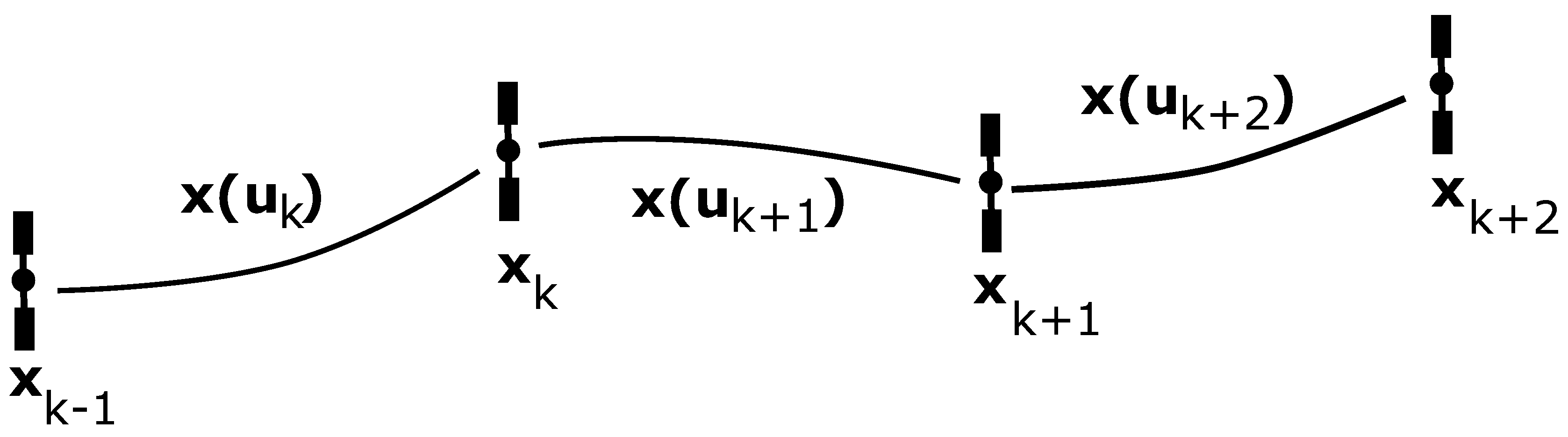
3.1. Fast and Slow Variable Considerations

The dynamic model described in the previous section are differential equations with respect to time. However, for the purpose of optimization, we reformulate the spacecraft dynamics as a set of differential equations representing the rate of change of slow variables with respect to the fast variable ϕ , as given below [39]:
d d ϕ h h X h Y e x e y T = 1 ϕ ˙ h ˙ h X ˙ h Y ˙ e x ˙ e y ˙ T
From Equation (1), we can see that the rate of change of angle ϕ with respect to time only depends on F h component of the thrust force acting on the spacecraft. We linearize the dynamic equations with respect to the out-of-plane thrust force component F h . We then obtain the following equations that represent the rate of change of spacecraft states (slow variables) with respect to the angle ϕ [39]:
d h d ϕ d h X d ϕ d h Y d ϕ d e x d ϕ d e y d ϕ h 3 μ 2 B 2 C F r F n F h + h 7 h Y sin ϕ m μ 5 h 2 h Y 2 B 5 C F r F h F n F h F h 2

3.2. Direct Transcription and Collocation

The optimization sub-problem is solved over each revolution, utilizing direct transcription and collocation. The trajectory for the k-th revolution is discretized into ( n 1 ) segments utilizing n nodes. The first-order differential Equations (7) with respect to the angle ϕ represent the spacecraft dynamics under the action of the thrust force are converted into a set of algebraic equations using the trapezoidal rule. The change of states of spacecraft from j t h node to ( j + 1 ) t h node where j ( 1 , 2 . . . . , n 1 ) can be computed as follows [39]:
h ˜ j , j + 1 h ˜ X j , j + 1 h ˜ Y j , j + 1 e ˜ x , j , j + 1 e ˜ y j , j + 1 Φ j + 1 ϕ j 2 d h d ϕ d h X d ϕ d h Y d ϕ d e x d ϕ d e y d ϕ j + d h d ϕ d h X d ϕ d h Y d ϕ d e x d ϕ d e y d ϕ j + 1
Using Equation (9), the change in orbital states over each segment of the orbit for one revolution are calculated. The change in the states after one complete revolution are calculated by summing the change of states across all segments, as given below [39]:
h h X h Y e x e y E N D T = h h X h Y e x e y T + j = 1 n 1 h ˜ j , j + 1 h ˜ X j , j + 1 h ˜ Y j , j + 1 e ˜ x , j , j + 1 e ˜ y j , j + 1
During the revolution, the magnitude of thrust generated is determined by the consideration of eclipses and the evaluation of the thruster efficiency, while the thrust direction (given by angles α and β ) is determined by solving the optimization sub-problem.

3.3. Trajectory Segments in Eclipses

During the transfer, whenever the spacecraft passes through the shadow of the Earth, it coasts in the absence of solar power to drive the onboard electric propulsion system. Hence, we need to identify the trajectory segments which are in the shadow of the Earth. We assume that the geometry of the shadow to be an infinitely long cylinder, with the radius being equal to that of the Earth. In this paper, we ignore the rotation of the Earth about the Sun, thereby assuming that the orientation of the eclipse does not change over time. To determine the trajectory segments that are in the shadow of the Earth, the inertial positional coordinates are computed at each node: with X-component being X j , Y-component being Y j and Z-component being Z j , and calculated for all nodes j ( 1 , 2 . . . . n ) during the revolution under consideration. Subsequently, we denote the set of segments that are in eclipses by T E and define it as follows [39]:
T E = { X j , X j + 1 > 0 a n d Y j 2 + Z j 2 , Y j + 1 2 + Z j + 1 2 R E 2 } [ X j Y j Z j ] T R 3 j ( 1 , 2 . . . . , n 1 )
Segments that belong to the set T E have zero thrust and the rate of change of states x of the spacecraft across these segments is considered to be zero.

3.4. Relative Thrust Efficiency

The relative thrust efficiency helps identify the segments of the discretized trajectory, where the spacecraft should coast (meaning that the thrust magnitude is zero). The trajectory over that segment is a conic section in the absence of orbital perturbations. The thruster efficiency is a measure of how effectively thrust force can influence the rate of change of the objective function. To this end, let us associate with each node the function f that provides the measure of the objective function computed at that node (instead of at the end of the revolution):
f j = min w 1 h j h G E O 2 + w 2 h X j + h Y j 2 + w 3 e x j + e y j 2
The function f is determined for each node within the optimization sub-problem and the objective function of the optimization sub-problem given in Equation (4) is determined at the end of the each revolution. The rate of change of the function f across the segment j , j + 1 of the discretized trajectory is given by:
f j f j + 1 f j ϕ j + 1 ϕ j .
The minimum and maximum rate of change of the function, taking into account all segments along the discretized trajectory over the revolution, can then be written as follows:
f min = min j f j , f max = max j f j .
The thrust efficiency is a measure of how well the thrust impacts the change in the objective function (f) by comparing the induced rate of change of the objective function ( f ). Considering the above, we define the metric relative thrust efficiency for a segment j , j + 1 as:
η j , j + 1 = f j f min f max f min .
We define a threshold value η T for the thruster efficiency. If the η j , j + 1 for the segment j , j + 1 is less than the threshold value, that is, if η j , j + 1 < η T , then the spacecraft will simply coast along the trajectory segment between the two nodes j and j + 1 . The relative thrust efficiency values range between 0 and 1. The set T η is then formed by identifying the segments where the spacecraft should coast, based on the user-defined threshold value of relative thrust efficiency ( η T ), as shown below:
T η = { j , j + 1 η j , j + 1 < η T , η j , j + 1 0 1 } , where j { 1 , 2 . . . . , n 1 } .

3.5. Optimization Sub-Problem

For the k-th revolution under consideration, the spacecraft thrust magnitude is determined by checking eclipse and thruster efficiency constraints. Specifically, the spacecraft thrusts in a segment where there is no eclipse and relative thrust efficiency is greater than the relative thrust efficiency threshold ( η T ). The spacecraft coasts along the remaining segments during that revolution. The thrust scheme can therefore be summarized as follows:
F j , j + 1 = 0 , if the segment j , j + 1 T E T η , F a v , k , otherwise .
The set T E of segments that remain in the eclipse are identified and the optimization sub-problem is solved using Matlab fminunc in order to identify the angles α and β for each Sun-lit segment on the trajectory. Next, the relative thrust efficiency is evaluated at all nodes and the set T η of segments where the spacecraft should not thrust are identified. We then determine the thrust magnitude across all segments using Equation (17). The computed state variables x at the end of the revolution serve as the starting conditions for the optimization sub-problem for the k + 1 revolution. Note that the mass of the spacecraft at the end of the revolution can be written as follows [39]:
m E N D = m F ( ϕ j + 1 ϕ j ) 2 I s p g 0 j , j + 1 T E T η ( h 3 μ 2 B j 2 + h 3 μ 2 B j + 1 2 + h 7 h Y sin ϕ j F sin β j m μ 5 h 2 h Y 2 B j 5 + h 7 h Y sin ϕ j + 1 F sin β j + 1 m μ 5 h 2 h Y 2 B j + 1 5 )

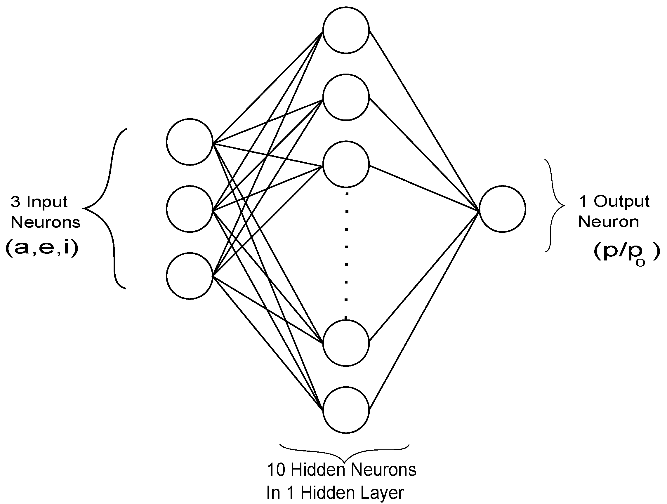
3.6. Neural Network for Predicting Power Loss

We propose to use an artificial neural network (ANN) to predict the power loss during each revolution of the low-thrust orbit-raising trajectory. An ANN is primarily a modelling technique that correlates various input and output data by changing the associated weights until a desired performance goal is met. Key parameters for developing an ANN are the number of hidden layers, number of neurons in the hidden layer and the activation functions used for normalizing the training data. The input to the neural network is given by set of the orbital elements z = a , e , i that can be derived from the state variables utilized in this paper. The output of the neural network is considered to be the power degradation due to radiation dose experienced by a spacecraft during one time period, considering a specific type of solar cell technology, as well as the type and amount of shielding for the solar arrays. For a network with a single hidden layer as shown in Figure 4, the predicted single output or power loss due to degradation in our case is defined as:
P ^ D = f 2 H 2 f 1 H 1 z + b 1 + b 2 ,
where H 1 and H 2 are weight matrices associated with input-hidden layer and hidden-output layer, respectively. These matrices have dimensions of n h × m i and 1 × n h , respectively. Here, m i is the number of inputs and n h is the number of nodes in the hidden layer, b 1 is the bias matrix of the hidden layer with dimensions n h × 1 , b 2 is a bias term for the output layer and is a scalar because the ANN has only one output, f 1 and f 2 represent the activation functions used for the hidden and output layers, respectively. The activation functions provide element-wise nonlinearities to the network [45]. There are various types of activation functions such as sigmoid, ReLU, tanh, etc., which are chosen based on the complexity of the data being trained. The characteristics of the network depends on the associated weights between the neurons of two consecutive layers. At first, the inputs are propagated through the network layers with initial weights to obtain an output. Based on the error between the predicted and the desired target output, the weights are updated after each iteration through back-propagation until the error is minimized or reaches a predetermined limit. In general, the mean squared error is considered as the measuring tool for network performance, where
M S E = 1 n i = 1 n P ^ D i P D i 2 .
Here, P ^ D i and P D i are the predicted and actual output values (power loss due to solar array degradation) respectively for the i-th training data point, with n being the total training points. The training is stopped after the defined performance criteria is met, that is, the mean-square error is within a preset tolerance value.

3.7. Neural Network Training of Radiation Data

In this section, the neural network training of the radiation data obtained from the AE9/AP9 tool, SPENVIS, and the overall training method is discussed. The training procedure begins with the creation of the power loss database due to proton dose. In our study for a test case scenario of GTO to GEO transfer, a small database is created depicting the power degradation for proton dose while varying the semi-major axis (a), eccentricity (e), and orbit inclination (i). The AE9/AP9 tool which is developed by the Air Force Research Laboratory (AFRL) is utilized alongside the SPENVIS tool developed by the European Space Agency (ESA) to create the database for proton dose and corresponding power degradation. In the AE9/AP9 tool, classical orbital elements are used to specify the orbits and ephemeris time range is taken as one day (1 March 2020 to 2 March 2020). Twenty-five different proton energy levels ranging from 0.1–2000 MeV are used for computing the proton dose. The models are run in perturbed mean mode with 95 percent setting for all energy levels. Shield material is selected as silicon dioxide with a depth of 4 mils. The database consisted of GTO with 24 different eccentricities and orbital altitudes while varying the inclination. With proton dose being calculated for the different orbits, we can estimate the solar cell power degradation using Equation (5). To this end, we assumed the cells to be ‘Azur 3G30’, a third generation triple junction (GaInP/GaAs/Ge) based semiconductor cell. Note here that the type of material of the solar cells and their shielding affect the radiation dose incurred during the transfer. Different materials are in use or are in development for onboard application [51,52]; the material used here represents state-of-the-art solar cell technology. A change in the material will require new training of the neural network; however, the methodology proposed here will remain the same. The empirical constants A , C, and D x for the triple junction solar cell, under consideration in this paper, are found to be 1, 0.306, and 3.63 × 10 9 MeV/g, respectively [53]. For orbits with high altitudes, damage dose will start to decrease as the inner Van Allen belt is mostly prominent in the vicinity of LEO and MEO. For predicting the power loss due to radiation, the ANN was created using nntool toolbox of Matlab software.
The radiation database input is taken in the form of (3 × 1) matrix of a, e, and i for 24 different orbits. The range of orbital eccentricities is taken between 0 to 0.73 while the inclination is varied across 0 to 30 degrees. The perigee altitude for the orbits ranged from 250 km to 35,786 km, while, for apogee altitude, it ranged between 35,786 km and 41,500 km. From the neural network architecture, as shown in Figure 5, we can define the dimensions of the weight and bias matrices. For our network, the weight matrices H 1 , H 2 had dimensions of (10 × 3) and (1 × 10), respectively, whereas the bias b 1 , b 2 has dimensions of (10 × 1) and (1 × 1). For the scale of the database under consideration, one hidden layer consisting of 10 neurons is sufficient. The generated database is eventually categorized into three sets to train the ANN: 70 percent being considered for training, 15 percent for testing, and the remaining 15 percent for validation. For normalizing the data, activation function softmax is selected for the hidden layer while it is considered to be tanh for the output layer. The Levenberg–Marquardt optimizer is used as training algorithm due to its rapid convergence rate [54]. Mean squared error is considered as the performance measuring tool of the network. In this case, the MSE turned out to be 0.001 which indicates that the data were well trained.

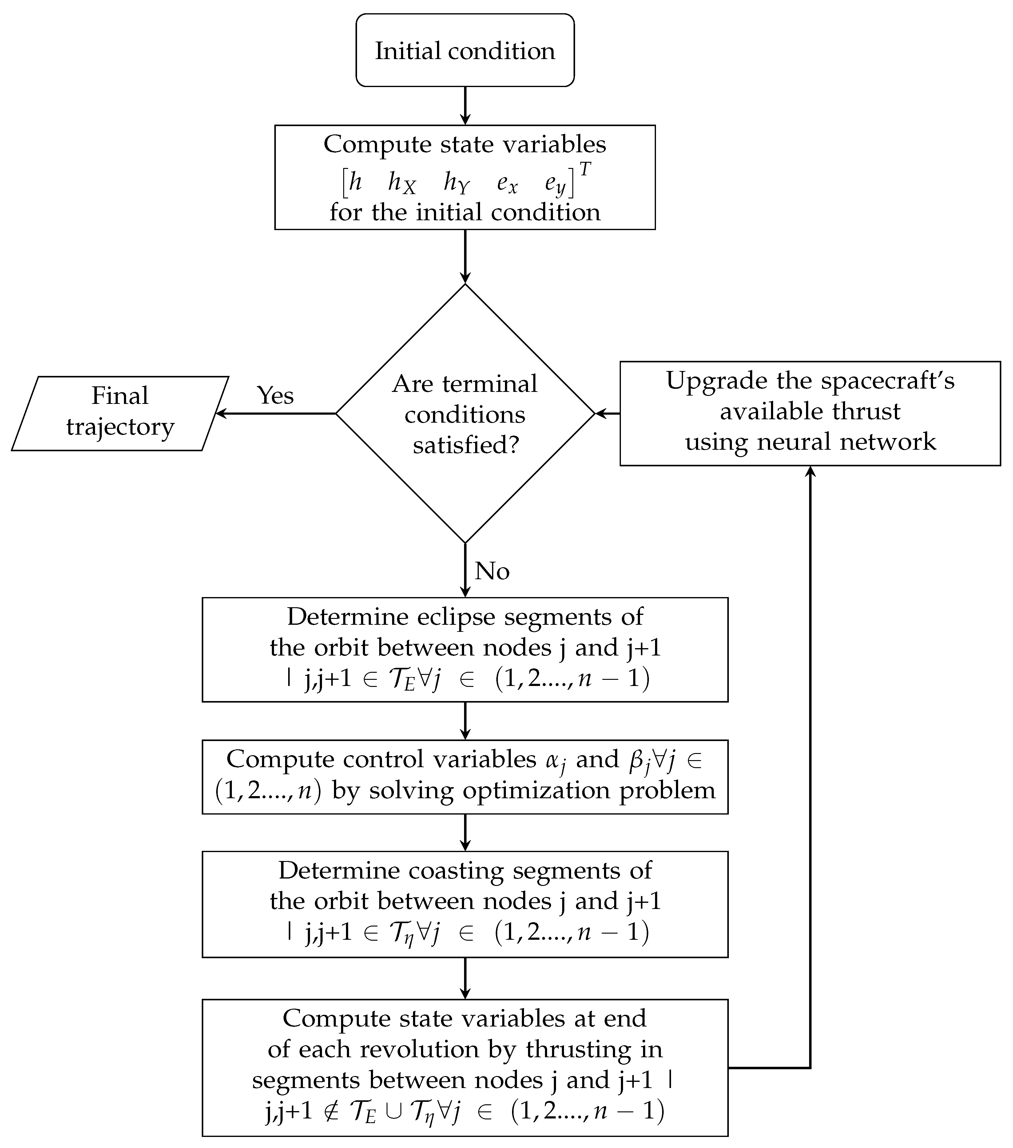
3.8. Optimization Tool Flow Chart

Figure 6 summarizes the developed optimization methodology. The spacecraft initial states are converted to the dynamic coordinates, from which the spacecraft trajectory is constructed by solving a sequence of optimization sub-problems. For each sub-problem, the segments within which the spacecraft is in the shadow of the earth is determined and the thrust available over these segments is set to zero. Each optimization sub-problem is solved using Matlab to determine the control variables α and β for each segment where the available thrust is positive. Next, inspection of thruster efficiency over the segments of the trajectory identifies when the spacecraft should turn off the thrusters to reduce the fuel expenditure. We then compute the end states of the spacecraft by summing up the effect of thrust force (magnitude and direction) over all segments. At the end of each revolution, the states of the spacecraft are used to determine the power degradation of solar cells using the neural network, and thereby the available thrust for the next revolution. The sequence of optimization sub-problems is solved until the terminal conditions are satisfied.

4. Numerical Results

In this section, the simulations with different initial conditions are used to compare the effect of various parameters associated with the algorithm. All the simulations are done by non-denationalizing the states of the spacecraft. The non-dimensional distance unit (1 DU) is equal to the radius of the GEO. The time unit (1 TU) is computed such that the gravitational constant is 1 DU 3 / 1 TU 2 . The mass unit (1 MU) is set to the initial mass of the spacecraft. The objective function is minimized using fminunc solver of MatLab. The optimization solver is run using the quasi-Newtonian algorithm for smaller computational times, but, in the final revolutions when the spacecraft is close to the GEO, the algorithm may fail to satisfy the end constraints and start oscillating. To avoid these oscillations, the optimization solver algorithm is switched to the Trust-Region algorithm when the spacecraft is close to the GEO. The initial mass of the spacecraft is 5000 kg and has an engine that has four BPT-4000 thrusters firing simultaneously providing a maximum thrust capacity of 1.16 N with a specific impulse of 1788 s. Note that the radiation damage in Van Allen belts will change this thrust capability as the transfer progresses. The simulation with no coasting is done with the spacecraft thrusting everywhere except for the eclipse portion of the orbit. The relative thrust efficiency for the thrusting mode simulation is set to 0.05, that is, the spacecraft does not thrust in the portion of the orbit where the relative thrust efficiency is less than 0.05 and in eclipses. All the algorithms are run on a machine using macOS Catalina on Intel i9 2.3 GHz processor (Wichita, KS, USA) with 8 Cores and 16 GB RAM.

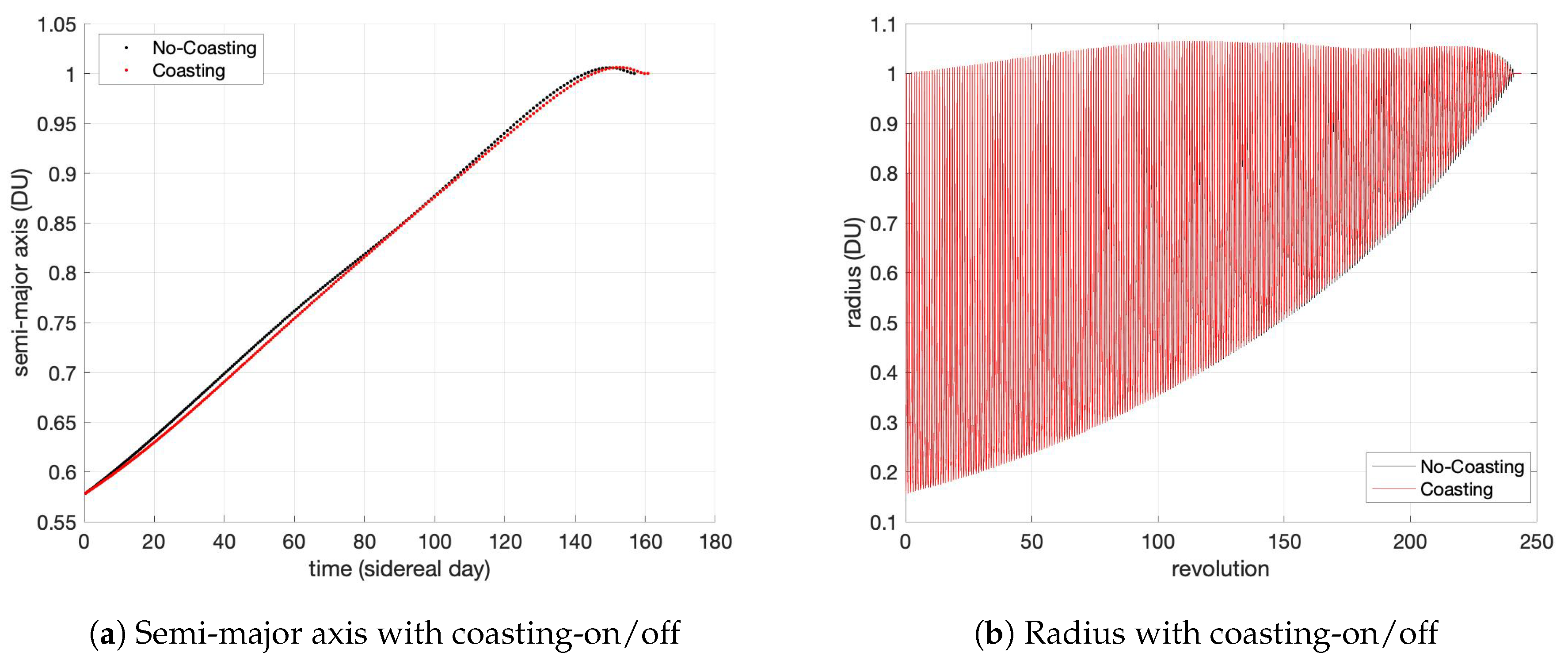
4.1. Transfer from GT0 to GEO

In this case, we use the GTO with perigee altitude of 250 km and inclination of 28.5 deg as the initial orbit. The time of the transfer has increased from 155.91 days to 160.81 days with allowance for coasting. The final mass of the spacecraft with no coasting was 4132.28 kg, whereas with coasting, it has increased to 4140.35 kg. The spacecraft has arrived in the final orbit making 225 revolutions with thrusting continuously except for eclipses and made 232 revolutions with coasting. The computational time for the algorithm with coasting mode on is 7.87 s that is slightly higher than the computational time of 7.81 s with coasting mode off. This increase in the computational time is for the additional computation of rate of change of objective function for the coasting mode on and for the additional optimization sub-problems solved for the transfer with an increase in the number of revolutions for the entire trajectory with the coasting. Results from the trajectory optimization algorithm are compared for coasting and no-coasting modes in Table 1.
In Figure 7, the trajectories and the optimal control angles of the spacecraft from GTO to GEO with both coasting ON/OFF are shown. The red color portion of the trajectory is where the spacecraft is coasting and the blue portion of the orbit is where the spacecraft is in the shadow of the Earth. The spacecraft thrusts in the black portion of the trajectory. The various osculating orbital parameters of the spacecraft with coasting ON/OFF at the end of each revolution are compared in Figure 8.
The plots for α and β angles in Figure 7 fluctuate between π to π . If the attitude dynamics and control system (ADCS) of the satellite are in charge of the thrust vectoring of the spacecraft, then it is important to investigate the variation of the control angles with respect to time, and ensure the changes are not drastic. Hence, we consider the change in angles α and β for continuously thrusting spacecraft over two revolutions; these variations are depicted in Figure 9. The change in α is always smooth as π and π are the same physically. In the case of β , there is a change in the angle from π / 2 to π / 2 . However, this change takes place over time in the magnitude of hours, allowing for enough time to ensure requisite thrust vectoring.

4.2. Transfer from Sub-GT0 to GEO

In this example, the Sub-GTO with a perigee altitude of 250 km and inclination of 28.5 deg is used as the initial orbit for the simulation. Similar to the previous example, this simulation also compares spacecraft trajectories with coasting when the relative thrust efficiency is below 0.05 and no coasting at all. In this simulation, it is observed that with the coasting the transfer time and revolutions made for the entire transfer increase as expected, but the final mass of the spacecraft has decreased slightly. Without coasting, the spacecraft final mass was 4105.74 kg, and, with coasting, the mass has decreased to 4104.83 kg. Note that the coasting strategy of spacecraft is evaluated during each revolution aimed at reducing the fuel expenditure for that revolution. However, the coasting also increases the number of revolutions made by the spacecraft considering the entire transfer; this leads to a slight decrease in the final mass of the spacecraft in some values of the relative thrust efficiency threshold values, and is further analyzed in Section 4.4. The transfer time with coasting is 167.55 days, while, without coasting, the spacecraft completes the transfer in 161.60 days. The transfer with coasting has made 276 revolutions and, without coasting, 265 revolutions are made. The computational time for the algorithm with coasting mode off is 9.30 s. The computational time of the algorithm with coasting being 10.39 s is more compared to the computational time of the algorithm with no coasting for the same reasons as discussed in Section 4.1. Table 2 shows the comparison of algorithm performance parameters for coasting ON/OFF modes.
The trajectories and the control angles of the spacecraft from Sub-GTO to GEO with both coasting ON/OFF are shown in Figure 10. Similar to the previous simulation, the red color portion of the trajectory is for coasting and the blue portion of the orbit is for the eclipse. The spacecraft thrusts in the black portion of the trajectory. Figure 11 depicts various osculating orbital parameters of the spacecraft with coasting ON/OFF.

4.3. Transfer from Super-GTO to GEO

In this simulation, initial orbit is considered as the super-GTO with perigee altitude of 250 km and inclination of 28.5 deg. The final mass of the spacecraft with coasting is 4175.53 kg and without coasting the spacecraft reaches the GEO with a final mass of 4165.99 kg. The entire transfer took 154.15 days with coasting and 150.08 days without coasting to complete. The spacecraft has done 192 revolutions while coasting and 193 revolutions without coasting before reaching their desired terminal states. The revolution made by the spacecraft without coasting is higher than when it was coasting, but the final transfer time is greater for the case when the spacecraft is coasting. The computational time for the super-GTO case is less than the above two simulations since the total number of optimization sub-problems to solve are less in number. Algorithm performance results in Table 3 provide the comparison for coasting ON/OFF modes of the transfer.
The trajectories and the control angles of the spacecraft from Super-GTO to GEO with both coasting ON/OFF are shown in Figure 12. As mentioned above, the red color portion of the trajectory is where the spacecraft is coasting and the blue portion of the orbit is where the spacecraft is in the shadow of the Earth. The spacecraft thrusts in the black portion of the trajectory. The various osculating orbital parameters of the spacecraft with coasting ON/OFF modes are compared in Figure 13.

4.4. Variations with Respect to the Thrust Efficiency Threshold

In this section, we discuss the variations of the algorithm’s performance parameters when coasting mode is ON with respect to the thrust efficiency threshold. The simulations are done by varying the thrust efficiency threshold values at a step of 0.1 from 0 to 0.9. In each case, the spacecraft thrusts in the portion of the orbit where the rate of change of the objective function is greater than the thrust efficiency threshold considered for that simulation. Figure 14 shows the corresponding plots of algorithm performance parameters with respect to the relative thrust efficiency threshold for transfers to GEO from GTO, Sub-GTO, and Super-GTO as initial orbits. The transfer time and the number of revolutions in the entire trajectory increase with the relative thrust efficiency threshold as expected. The final mass of the spacecraft tends to increase with the relative thrust efficiency threshold value. However, in some cases, the final mass of the spacecraft reduces with a slight increase in the relative thrust efficiency threshold. This is because the relative thrust efficiency threshold determines the coasting portions of the orbit for each revolution. This will minimize fuel spent by the spacecraft for that revolution, but it will also make the spacecraft do more revolutions to reach the final orbit. In some cases, the fuel spent by the spacecraft for thrusting those extra revolutions is more than the fuel saved due to the coasting. The analysis shown here can help us understand in choosing the user-defined relative thrust efficiency threshold value for the low thrust orbit raising trajectory design.

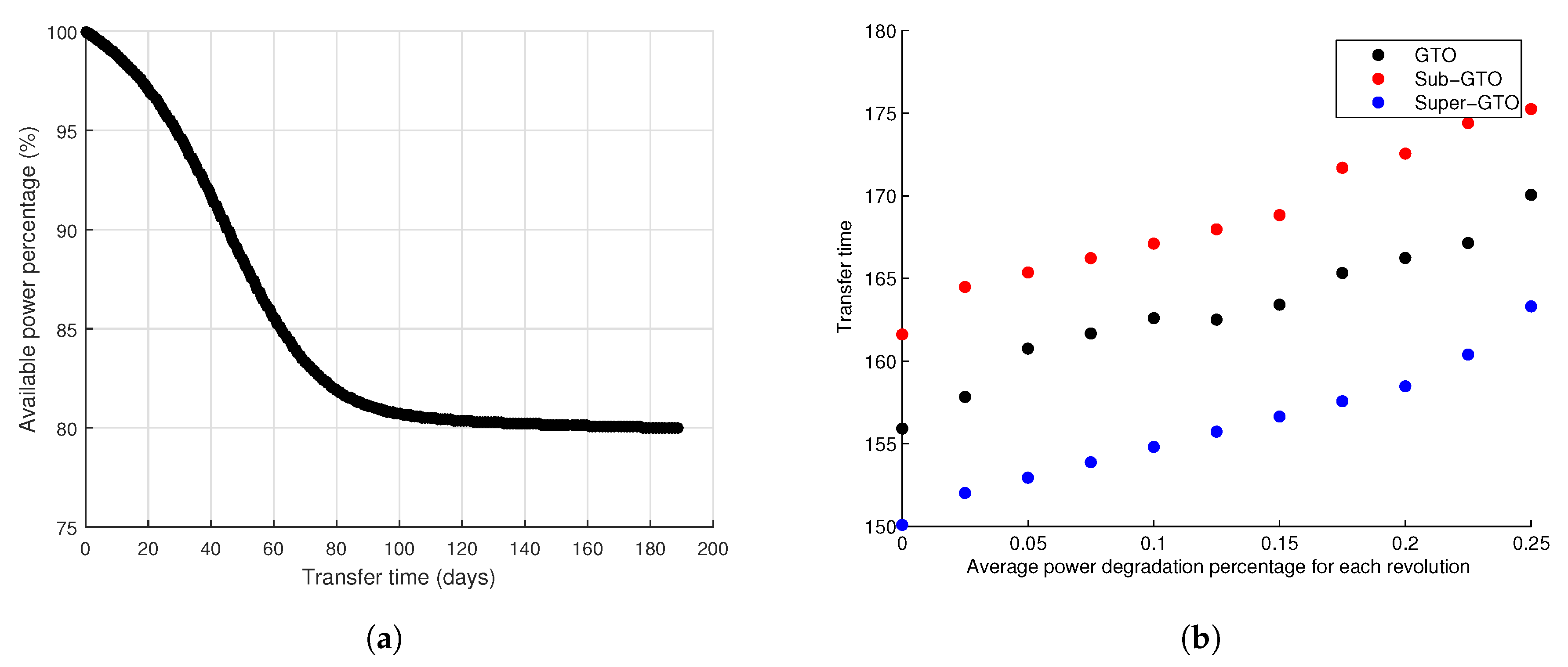
4.5. Power Degradation Due to Radiation

In this section, power degradation due to radiation effect on the solar arrays of the spacecraft with 4 mil shielding, predicted by the neural network is analyzed. To this end, the trajectories to GEO from GTO with a perigee altitude of 250 km and inclination of 28.5 deg are determined with degrading thrust due to radiation and the coasting-ON. The transfer time with the degrading thrust is increased to 188.72 days from 160.81 days. The decrease in the thrust makes the spacecraft less maneuverable and increases the time to reach GEO. The final mass of the spacecraft with degrading thrust is 4131.91 kg and with constant thrust is 4140.35 kg. The spacecraft made 267 revolutions before reaching the GEO with degrading thrust due to the radiation and 232 revolutions with constant trust. In both simulations, the spacecraft is coasting with the relative thrust efficiency threshold value set as 0.05. Important parameters of the trajectory optimization algorithm are compared for constant and degrading thrust in Table 4.
The trajectories and the control angles of the spacecraft from GTO to GEO with coasting ON using constant and degrading thrusts are shown in Figure 15. The red color portion of the trajectory is for coasting and the blue portion of the orbit is for the eclipse. The spacecraft thrusts in the black portion of the trajectory. The portions of the orbit where the spacecraft coasts are similar for both the cases irrespective of the magnitude of thrust available to the spacecraft. Figure 16 compares various osculating orbital parameters of the spacecraft for constant and degrading thrusts.
Figure 17 shows the power degradation prediction of the neural network from GTO to GEO with respect to the transfer time. Initially, the power degradation is high as the spacecraft passes through the Van-Allen belts and, when the spacecraft reaches higher altitudes, the power remains almost the same. The available power is degraded by approximately 20 percent by the time the spacecraft reaches GEO. The transfer time has increased compared to the transfer to GEO without power degradation due to the decrease in the available thrust with each revolution. The power degradation due to radiation is compared with a similar orbit-raising mission scenario presented in Ref. [53], in which case the remaining power after the transfer turned out to be 81.9 percent of the beginning-of-life power. Our degradation computation is close (79.98 percent), and the difference is likely due to the difference in maneuvering strategies.
We now consider a variety of orbit-raising mission scenarios to investigate the average power degradation for each revolution defined as the ratio of total power degradation during the transfer to the number of revolutions made by the spacecraft before it passes through the Van Allen radiation belts. Figure 17 shows the increase in the transfer time by considering the average power degradation for each revolution until the spacecraft passes through the Van Allen radiation belts for transfers from GTO, Sub-GTO, and Super-GTO. The plot shows that the average power degradation is lower when the spacecraft starts the transfer from super-GTO, owing to comparatively larger portion of each revolution being outside the most hazardous parts of the Van Allen belts.

5. Conclusions

In this paper, we consider geocentric electric orbit-raising problem, modeled as a sequence of orbit-raising sub-problems, with the goal of the minimizing the deviation from the geosynchronous equatorial orbit in each revolution. The use of a recently developed model for the spacecraft translational dynamics, along with the sequential optimization procedure, allows for fast and robust computation of orbit-raising trajectories. This paper extended the mathematical formulation in two different ways: allowance for coasting beyond the shadow of the Earth and provision of computation of power loss of the solar arrays and thereby the available thrust for the remaining part of the transfer. The first extension is performed by incorporating the concept of thruster efficiency within the optimization sub-problem; a threshold on the thruster efficiency allows for the identification of trajectory segments, outside the shadow of the Earth, where the spacecraft coasts. The second extension incorporates an artifical neural network within the optimization framework; this neural network computes the solar array power loss after the end of a revolution, and updates the available thrust for the next revolution of the transfer. The neural network is trained offline on AP9 and SPENVIS generated data for different orbits. AP9 provides the incident proton spectra along these orbits, and SPENVIS utilizes the non-ionizing energy loss calculations to compute the displacement damage dose, and therefore the power loss. A variety of orbit-raising mission scenarios starting from different geosynchronous transfer orbits (GTO) have been considered to investigate the effects of thruster efficiency on the mass of the deployed satellite and the transfer time of the orbit-raising maneuver. We also studied the average power degradation encountered during the transfer from these various orbits. It was found that transfers starting from super-GTO result in smaller fuel expenditure (larger deployed mass) and lower average power degradation compared to the GTO and sub-GTO counterparts. Importantly, the use of a neural network to compute the power loss has minimal impact on the computational time for the overall trajectory design. In fact, numerical simulations for the considered mission scenarios demonstrate that the proposed extensions do not impede the fast and robust nature of the tool under consideration.

Author Contributions

Conceptualization, A.D.; methodology, P.C. and T.F.; software, P.C. and T.F.; validation, P.C., T.F. and A.D.; formal analysis, P.C. and T.F.; investigation, P.C., T.F. and A.D.; resources, A.D.; data curation, P.C. and T.F.; writing–original draft preparation, P.C. and T.F.; writing–review and editing, P.C., T.F. and A.D.; visualization, P.C. and T.F.; supervision, A.D.; project administration, A.D.; funding acquisition, N/A. All authors have read and agreed to the published version of the manuscript.

Funding

This research received no external funding.

Acknowledgments

We acknowledge the use of the following two software for creating the training data for the artificial neural network developed in the paper: AE9/AP9 Version V1.50.001 (https://www.vdl.afrl.af.mil/programs/ae9ap9/), and SPENVIS Version 4.6.10 (https://www.spenvis.oma.be/).

Conflicts of Interest

The authors declare no conflict of interest.

References

  1. Mazouffre, S. Electric propulsion for satellites and spacecraft: Established technologies and novel approaches. Plasma Sources Sci. Technol. 2016, 25, 033002. [Google Scholar] [CrossRef]
  2. Levchenko, I.; Bazaka, K.; Mazouffre, S.; Xu, S. Prospects and physical mechanisms for photonic space propulsion. Nat. Photonics 2018, 12, 649–657. [Google Scholar] [CrossRef]
  3. Van Loef, E.; Dorenbos, P.; Van Eijk, C.; Krämer, K.; Güdel, H.U. High-energy-resolution scintillator: Ce 3+ activated LaBr 3. Appl. Phys. Lett. 2001, 79, 1573–1575. [Google Scholar] [CrossRef]
  4. Levchenko, I.; Keidar, M.; Cantrell, J.; Wu, Y.L.; Kuninaka, H.; Bazaka, K.; Xu, S. Explore space using swarms of tiny satellites. Nature 2018, 562, 185–187. [Google Scholar] [CrossRef] [PubMed] [Green Version]
  5. Boeuf, J.P. Tutorial: Physics and modeling of Hall thrusters. J. Appl. Phys. 2017, 121, 011101. [Google Scholar] [CrossRef]
  6. Lemmer, K. Propulsion for cubesats. Acta Astronaut. 2017, 134, 231–243. [Google Scholar] [CrossRef]
  7. Lev, D.R.; Herscovitz, J.; Kariv, D.; Mizrachi, I. Heated gas propulsion system conceptual design for the Samson nano-satellite (propulsion). J. Small Satell. 2017, 6, 551–564. [Google Scholar]
  8. Feuerborn, S.A.; Perkins, J.; Neary, D.A. Finding a way: Boeing’s all electric propulsion satellite. In Proceedings of the 49th AIAA/ASME/SAE/ASEE Joint PropulsionConference, San Jose, CA, USA, 14–17 July 2013. [Google Scholar]
  9. Sembély, X.; Wartelski, M.; Doubrère, P.; Deltour, B.; Cau, P.; Rochard, F. Design and Development of an Electric Propulsion Deployable Arm for Airbus Eurostar E3000 ComSat Platform. In Proceedings of the 35th International Electric Propulsion Conference Georgia Institute of Technology, Atlanta, GA, USA, 8–12 October 2017. [Google Scholar]
  10. Huifeng, X. Space Development with Chinese Characteristics and its Practical Significance. Aerosp. China 2019, 19, 39–45. [Google Scholar]
  11. Lawden, D. Optimal Trajectories for Space Navigation; Butterworths: London, UK, 1963. [Google Scholar]
  12. Marasch, M.W.; Hall, C.D. Application of Energy Storage to Solar Electric Propulsion Orbital Transfer. J. Spacecr. Rockets 2000, 37, 645–652. [Google Scholar] [CrossRef] [Green Version]
  13. Ferrier, C.H.; Epenoy, R. Optimal Control for Engines with Electro-Ionic Propulsion under Constraint of Eclipse. Acta Astronaut. 2001, 48, 181–192. [Google Scholar] [CrossRef]
  14. Kluever, C.A. Geostationary Orbit Transfers Using Solar Electric Propulsion with Specific Impulse Modulation. J. Spacecr. Rockets 2004, 41, 461–466. [Google Scholar] [CrossRef]
  15. Kiforenko, B.N. Optimal low-thrust orbital transfers in a central gravity field. Int. Appl. Mech. 2005, 41, 1211–1238. [Google Scholar] [CrossRef]
  16. Russell, R. Primer Vector Theory Applied to Global Low-Thrust Trade Space Studies. J. Guid. Control Dyn. 2007, 30, 2. [Google Scholar] [CrossRef]
  17. Kluever, C.A.; Oleson, S.R. Direct approach for computing near-optimal low-thrust earth-orbit transfers. J. Spacecr. Rockets 1998, 35, 509–515. [Google Scholar] [CrossRef]
  18. Falck, R.; Dankanich, J. Optimization of Low-Thrust Spiral Trajectories by Collocation. In Proceedings of the AIAA/AAS Astrodynamics Specialist Conference, Guidance, Navigation, and Control and Co-located Conferences, Minneapolis, MI, USA, 13–16 August 2012. [Google Scholar]
  19. Dutta, A.; Libraro, P.; Kasdin, N.J.; Choueiri, E. A Direct Optimization Based Tool to Determine Orbit-Raising Trajectories to GEO for All-Electric Telecommunication Satellites. In Proceedings of the AAS Astrodynamics Specialist Conference, Minneapolis, MI, USA, 13–16 August 2012. [Google Scholar]
  20. Graham, K.F.; Rao, A.V. Minimum-Time Trajectory Optimization of Low-Thrust Earth-Orbit Transfers with Eclipsing. J. Spacecr. Rockets 2016, 53, 289–303. [Google Scholar] [CrossRef] [Green Version]
  21. Betts, J.T.; Campbell, S.L.; Thompson, K.C. Solving optimal control problems with control delays using direct transcription. Appl. Numer. Math. 2016, 108, 185–203. [Google Scholar] [CrossRef] [Green Version]
  22. Betts, J.T.; Campbell, S.L.; Digirolamo, C. Initial guess sensitivity in computational optimal control problems. Numer. Algebra Control Optim. 2020, 10, 31. [Google Scholar] [CrossRef] [Green Version]
  23. Edelbaum, T.N. Propulsion requirements for controllable satellites. ARS J. 1961, 31, 1079–1089. [Google Scholar] [CrossRef]
  24. Flandro, G.A. Asymptotic Solution for Solar Electric Low-Thrust Orbit Raising with Eclipse Penalty. In Proceedings of the AIAA Mechanics and Control of Flight Conference, Anaheim, CA, USA, 5–9 August 1974. [Google Scholar]
  25. Wiesel, W.; Alfano, S. Optimal Many-Revolution Orbit Transfer. J. Guid. Control Dyn. 1985, 8, 155–157. [Google Scholar] [CrossRef]
  26. Kechichian, J.A. Low-Thrust Eccentricity-Constrained Orbit Raising. J. Spacecr. Rockets 1998, 35, 327–335. [Google Scholar] [CrossRef]
  27. Kechichian, J.A. Orbit Raising with Low-Thrust Tangential Acceleration in Presence of Earth Shadow. J. Spacecr. Rockets 1998, 35, 516–525. [Google Scholar] [CrossRef]
  28. Kechichian, J.A. Low-Thrust Inclination Control in Presence of Earth Shadow. J. Spacecr. Rockets 1998, 35, 526–532. [Google Scholar] [CrossRef]
  29. Kluever, C. Simple Guidance Scheme for Low-Thrust Orbit Transfers. J. Guid. Control Dyn. 1998, 21, 1015–1017. [Google Scholar] [CrossRef]
  30. Petropoulos, A.E. Simple Control Laws for Low-thrust Orbit Transfers. In Proceedings of the AIAA/AAS Astrodynamics Specialist Conference, Big Sky Resort, Big Sky, MT, USA, 3–7 August 2003. [Google Scholar]
  31. Colasurdo, G.; Casalino, L. Optimal Low-Thrust Maneuvers in Presence of Earth Shadow. In Proceedings of the AIAA/AAS Astrodynamics Specialist Conference and Exhibit, Providence, RI, USA, 16–19 August 2004. [Google Scholar]
  32. Wall, B.; Conway, B. Shape-Based Approach to Low-Thrust Rendezvous Trajectory Design. J. Guid. Control Dyn. 2009, 32, 95–101. [Google Scholar] [CrossRef]
  33. Kluever, C. Using Edelbaum’s Method to Compute Low-Thrust Transfers with Earth-Shadow Eclipses. J. Guid. Control Dyn. 2011, 34, 300–303. [Google Scholar] [CrossRef]
  34. Taheri, E.; Abdelkhalik, O. Shape-Based Approximation of Constrained Low-Thrust Space Trajectories Using Fourier Series. J. Spacecr. Rockets 2012, 49, 535–545. [Google Scholar]
  35. Falck, R.D.; Sjauw, W.K.; Smith, D.A. Comparison of Low-Thrust Control Laws for Applications in Planetocentric Space. In Proceedings of the 50th AIAA/ASME/SAE/ASEE Joint Propulsion Conference, Cleveland, OH, USA, 28–30 July 2014. [Google Scholar]
  36. Betts, J.T. Optimal low–thrust orbit transfers with eclipsing. Opt. Control Appl. Methods 2015, 36, 218–240. [Google Scholar] [CrossRef]
  37. Kelchner, M.J.; Kluever, C.A. Rapid Evaluation of Low-Thrust Transfers from Elliptical Orbits to Geostationary Orbit. J. Spacecr. Rockets 2020. to appear, published online as Article in Advance. [Google Scholar] [CrossRef]
  38. Junkins, J.L.; Taheri, E. Exploration of Alternative State Vector Choices for Low-Thrust Trajectory Optimization. J. Guid. Control Dyn. 2019, 42, 47–64. [Google Scholar] [CrossRef]
  39. Sreesawet, S.; Dutta, A. Fast and Robust Computation of Low-Thrust Orbit-Raising Trajectories. AIAA J. Guid. Control Dyn. 2018, 41, 1888–1905. [Google Scholar] [CrossRef]
  40. Sreesawet, S.; Dutta, A. Receding Horizon Control for Spacecraft with Low-Thrust Propulsion. In Proceedings of the 2018 Annual American Control Conference (ACC), Milwaukee, WI, USA, 27–29 June 2018. [Google Scholar]
  41. Dutta, A.; Vijayan, S.; Olson, T. Deployment of High Power Class All-Electric Satellites in the Geosynchronous Equatorial Orbit. In Proceedings of the AIAA/AAS Astrodynamics Specialist Conference (AIAA SPACE Forum), Long Beach, CA, USA, 13–16 September 2016. [Google Scholar]
  42. Sreesawet, S.; Pappu, V.; Dutta, A.; Steck, J. Neural Networks Based Adaptive Controller for Attitude Control of All-Electric Satellites. In Advances in the Astronautical Sciences; Number AAS 15-754; Univelt: Vail, CO, USA, 2015. [Google Scholar]
  43. Chadalavada, P.S.; Dutta, A. Relative Equations of Motion using a New Set of Orbital Elements. Adv. Astronaut. Sci. 2018, 167, 565–581. [Google Scholar]
  44. Dutta, A.; Arora, L. Objective Function Weight Selection for Sequential Low-Thrust Orbit-Raising Optimization Problem. In Proceedings of the AIAA/AAS Space Flight Mechanics Meeting, Ka’anapali, Maui, HI, USA, 13–17 January 2019. [Google Scholar]
  45. Arora, L.; Dutta, A. Reinforcement Learning for Sequential Low-Thrust Orbit Raising Problem. In Proceedings of the AIAA Scitech 2020 Forum, Orlando, FL, USA, 6–10 January 2020. [Google Scholar]
  46. Petropoulos, A.E. Low-thrust Orbit Transfers Using Candidate Lyapunov Functions with a Mechanism for Coasting. In Proceedings of the AIAA/AAS Astrodynamics Specialist Conference, Providence, RI, USA, 16–19 August 2004. [Google Scholar]
  47. Dutta, A.; Libraro, P.; Kasdin, N.J.; Choueiri, E.; Francken, P. Minimum-fuel electric orbit-raising of telecommunication satellites subject to time and radiation damage constraints. In Proceedings of the 2014 American Control Conference, Portland, OR, USA, 4–6 June 2014; pp. 2942–2947. [Google Scholar]
  48. Kluever, C.A.; Messenger, S.R. Solar-Cell Degradation Model for Trajectory Optimization Methods. J. Spacecr. Rockets 2019, 56, 844–853. [Google Scholar] [CrossRef]
  49. Messenger, S.; Jackson, E.; Warner, J.; Walters, R. Scream: A new code for solar cell degradation prediction using the displacement damage dose approach. In Proceedings of the 35th IEEE Photovoltaic Specialists Conference, Honolulu, HI, USA, 20–25 June 2010; pp. 001106–001111. [Google Scholar]
  50. Dutta, A.; Kasdin, N.J.; Choueiri, E.; Francken, P. Minimizing proton displacement damage dose during electric orbit raising of satellites. J. Guid. Control Dyn. 2016, 39, 963–969. [Google Scholar] [CrossRef]
  51. Levchenko, I.; Bazaka, K.; Belmonte, T.; Keidar, M.; Xu, S. Advanced Materials for Next,-Generation Spacecraft. Adv. Mater. 2018, 30, 1802201. [Google Scholar] [CrossRef] [PubMed]
  52. Levchenko, I.; Xu, S.; Teel, G.; Mariotti, D.; Walker, M.; Keidar, M. Recent progress and perspectives of space electric propulsion systems based on smart nanomaterials. Nat. Commun. 2018, 9, 879. [Google Scholar] [CrossRef] [PubMed]
  53. Lozinski, A.R.; Horne, R.B.; Glauert, S.A.; Del Zanna, G.; Heynderickx, D.; Evans, H.D. Solar Cell Degradation Due to Proton Belt Enhancements During Electric Orbit Raising to GEO. Space Weather 2019, 17, 1059–1072. [Google Scholar] [CrossRef]
  54. Marquardt, D.W. An algorithm for least-squares estimation of nonlinear parameters. J. Soc. Ind. Appl. Math. 1963, 11, 431–441. [Google Scholar] [CrossRef]
Figure 1. A 225-revolution, 156-day low-thrust orbit-raising maneuver from GTO to GEO.
Aerospace 07 00074 g001
Figure 2. Control angles α and β representing the thrust directions in the reference frame N .
Aerospace 07 00074 g002
Figure 3. Low-thrust orbit-raising maneuver modeled as a sequence of optimization sub-problems.
Aerospace 07 00074 g003
Figure 4. A generalized artificial neural network architecture with a single hidden layer.
Aerospace 07 00074 g004
Figure 5. Schematic of the artificial neural network architecture used for the study.
Aerospace 07 00074 g005
Figure 6. Algorithm flow chart.
Aerospace 07 00074 g006
Figure 7. Trajectory and control angles of GTO-GEO.
Aerospace 07 00074 g007aAerospace 07 00074 g007b
Figure 8. Osculating orbital elements of GTO-GEO trajectory.
Aerospace 07 00074 g008aAerospace 07 00074 g008b
Figure 9. Variations of angles alpha and beta over two revolution during the transfer.
Aerospace 07 00074 g009
Figure 10. Trajectory and control angles of Sub-GTO to GEO transfer.
Aerospace 07 00074 g010aAerospace 07 00074 g010b
Figure 11. Osculating orbital elements of Sub-GTO to GEO trajectory.
Aerospace 07 00074 g011
Figure 12. Trajectory and control angles of Super-GTO to GEO transfer.
Aerospace 07 00074 g012aAerospace 07 00074 g012b
Figure 13. Osculating orbital elements of Super-GTO to GEO trajectory.
Aerospace 07 00074 g013
Figure 14. Performance parameters with coasting ON with respect to the thrust efficiency threshold.
Aerospace 07 00074 g014
Figure 15. Trajectory and control angles of GTO-GEO with coasting ON.
Aerospace 07 00074 g015
Figure 16. Osculating orbital elements of GTO-GEO trajectory with coasting ON.
Aerospace 07 00074 g016
Figure 17. (a) power degradation predicted using neural network; (b) transfer time vs. average power degradation for each revolution.
Aerospace 07 00074 g017
Table 1. Algorithm performance comparison for coasting ON/OFF modes for GTO to GEO transfer.
ParameterCoasting-ONCoasting-OFF
Final Mass4140.35 kg4134.28 kg
Transfer Time160.81 days155.91 days
Revolutions232225
Computational Time7.87 s7.81 s
Table 2. Algorithm performance comparison for coasting ON/OFF modes for Sub-GTO to GEO transfer.
ParameterCoasting-ONCoasting-OFF
Final Mass4104.83 kg4105.74 kg
Transfer Time167.55 days161.60 days
Revolutions276265
Computational Time10.39 s9.30 s
Table 3. Algorithm performance comparison for coasting ON/OFF modes for Super-GTO to GEO transfer.
ParameterCoasting-ONCoasting-OFF
Final Mass4175.53 kg4165.99 kg
Transfer Time154.15 days150.08 days
Revolutions192193
Computational Time5.6 s5.23 s
Table 4. Algorithm performance comparison with neural network and coasting mode ON for GTO to GEO transfer.
ParameterConstant ThrustDegrading Thrust
Final Mass4140.35 kg4131.91 kg
Transfer Time160.81 days188.72 days
Revolutions232267

